A generic risk based surveying method for invading plant pathogens

A generic risk­based surveying method for 

invading plant pathogens

Parnell, SR, Gottwald, TR, Riley, T and van den Bosch, F

http://dx.doi.org/10.1890/13­0704.1

Title

A generic risk­based surveying method for invading plant pathogens

Authors

Parnell, SR, Gottwald, TR, Riley, T and van den Bosch, F

Type

Article

URL

This version is available at: http://usir.salford.ac.uk/id/eprint/33453/

Published Date

2014

USIR is a digital collection of the research output of the University of Salford. Where copyright 

permits, full text material held in the repository is made freely available online and can be read, 

downloaded and copied for non­commercial private study or research purposes. Please check the 

manuscript for any further copyright restrictions.

A generic risk-based surveying method for invading plant pathogens

S. PARNELL,1,4T. R. GOTTWALD,2T. RILEY,3ANDF.VAN DENBOSCH1

1_{Rothamsted Research, Department of Computational and Systems Biology, Harpenden, Hertfordshire AL5 2JQ United Kingdom} 2

U.S. Department of Agriculture, Agricultural Research Service, Ft. Pierce, Florida 34945 USA 3_{U.S. Department of Agriculture, Animal and Plant Health Inspection Service, Orlando, Florida 32827 USA}

Abstract. Invasive plant pathogens are increasing with international trade and travel,

with damaging environmental and economic consequences. Recent examples include tree diseases such as sudden oak death in the Western United States and ash dieback in Europe. To control an invading pathogen it is crucial that newly infected sites are quickly detected so that measures can be implemented to control the epidemic. However, since sampling resources are often limited, not all locations can be inspected and locations must be prioritized for surveying. Existing approaches to achieve this are often species specific and rely on detailed data collection and parameterization, which is difficult, especially when new arrivals are unanticipated. Consequently regulatory sampling responses are often ad hoc and developed without due consideration of epidemiology, leading to the suboptimal deployment of expensive sampling resources. We introduce a flexible risk-based sampling method that is pathogen generic and enables available information to be utilized to develop epidemiologically informed sampling programs for virtually any biologically relevant plant pathogen. By targeting risk we aim to inform sampling schemes that identify high-impact locations that can be subsequently treated in order to reduce inoculum in the landscape. This ‘‘damage limitation’’ is often the initial management objective following the first discovery of a new invader. Risk at each location is determined by the product of the basic reproductive number (R0), as a measure of local epidemic size, and the probability of infection. We illustrate how

the risk estimates can be used to prioritize a survey by weighting a random sample so that the highest-risk locations have the highest probability of selection. We demonstrate and test the method using a high-quality spatially and temporally resolved data set on Huanglongbing disease (HLB) in Florida, USA. We show that even when available epidemiological information is relatively minimal, the method has strong predictive value and can result in highly effective targeted surveying plans.

Key words: citrus plantings, Florida, USA; early detection; epidemic; Huanglongbing disease; invasive species; landscape epidemiology; monitoring; pathogen risk; surveillance.

INTRODUCTION

The global movement of plants and plant products has increased rapidly in recent times with an associated increase in the number of introduced plant pathogens (Jones and Baker 2007, Brasier 2008). Exotic pathogens often face little natural resistance outside their native ranges and so have caused severe environmental and economic damage in natural and cultivated plant communities. A prominent example is sudden oak death (causal agentPhytophthora ramorum), which has caused extensive environmental damage to woodland commu-nities in the western Uniited States since its introduction in 1995 (Rizzo and Garbelotto 2003) and currently poses a significant threat to heathland and woodland environ-ments in the United Kingdom (Brasier et al. 2004). Another example is ash dieback (Chalara fraxinea), a damaging fungal disease that has recently invaded a

number of countries in Europe (Kowalski 2009, Chandelier et al. 2011, Husson et al. 2011, Timmermann et al. 2011, Baric et al. 2012, Bengtsson et al. 2013), prompting the rapid deployment of extensive surveying and control resources (Anonymous 2012a). Following the first discovery of an invading plant pathogen a regulatory agency must act quickly to mitigate the problem since management becomes disproportionately more costly and difficult with increasing pathogen incidence. However, the large-scale spatial and temporal dynamics of an invasive pathogen spreading through a heterogeneous landscape are difficult to predict. Detect-ing new positive sites is therefore challengDetect-ing and requires the deployment of extensive surveying resourc-es, at great cost.

A large body of work has focused on methods to inform surveying programs for invasive species detec-tion. These studies have made significant progress in terms of incorporating environmental and population-level information to accurately predict species distribu-tion (Allouche et al. 2006, Inglis et al. 2006, Austin 2007, Va´clavik and Meentemeyer 2009, 2012, Williams et al.

Manuscript received 16 April 2013; revised 23 August 2013; accepted 5 September 2013. Corresponding Editor: R. A. Hufbauer.

4_{E-mail: [email protected]}

2009), which in turn can be used to target surveying programs (Crall et al. 2013). However, many of these methods depend upon extensive species-specific model development and data collection. For many potential plant pathogen threats this is not possible, since many new arrivals are unanticipated and the state of epidemiological knowledge available varies widely from species to species. There is thus a need for a more general method that can incorporate the available epidemiological information to improve survey effec-tiveness and facilitate the rapid emergency development of sampling plans. The lack of such a method means that in practice regulatory sampling plans are ad hoc and can result in the suboptimal deployment of finite and expensive sampling resources. Any improvement in the efficiency to detect new positive sites will save sampling resources as well as increase the likelihood of success of the management program.

In this paper we propose a risk-based sampling method aimed at identifying high-risk locations in a landscape and targeting control resources for inoculum reduction and disease containment. The method has been adopted in practice by the USDA (U.S. Depart-ment of Agriculture) and Defra (DepartDepart-ment for Environment, Food, and Rural Affairs, UK) for different pathosystems. The aim of this paper is to present the general method and validate it based on available data. By framing our approach around an epidemiologically motivated definition of risk we pro-vide a generic method that allows available information to be incorporated in a clear mechanistic way. For some invasive pathogens the biological parameters will be well known from previous epidemics or from epidemics in similar host regions. However, for many invasive pathogens little epidemiological information is available as they are either novel emerging species or are invading a novel environment. Thus, we analyze two distinct scenarios that may confront a regulatory agency: either (1) the biological parameters associated with risk are known, or can be inferred from expert opinion, or (2) the parameters are not known and therefore must be estimated using the survey data. We illustrate the method using an epidemic of a bacterial pathogen of citrus that is the causal agent of Huanglongbing (HLB) (syn. ‘‘Citrus Greening’’) in Florida, USA (Gottwald 2010). Although we use a crop-tree example to test the method, due to the availability of a high-quality spatially and temporally resolved data set, the method equally lends itself to nonagricultural applications in natural and seminatural landscapes.

MATERIALS ANDMETHODS

In this section we describe how estimates of pathogen risk can be derived for different host locations within a landscape. We describe a straightforward way to parameterize and validate the method, and then suggest an approach that can be taken by a practitioner to use the estimates of risk to determine a sampling program, i.e.,

risk-weighted random sampling. Finally, we demonstrate the method by means of a specific example, an epidemic of citrus HLB (Huanglongbing) in Florida, USA.

Calculating risk

The purpose of the method is to determine spatially referenced estimates of risk that can be used to inform targeted sampling plans in a host landscape. The individual spatial unit we associate with risk is a ‘‘host location.’’ We define a host location as ‘‘any relatively homogenous area of discrete habitat that contains plants susceptible to the pathogen’’; for example, this could be an individual plant or a collection of plants in a host location. The risk associated with a host location is defined as the product of (1) the expected local-epidemic size if the pathogen were to arrive and (2) the probability that the pathogen arrives and causes an epidemic at that location,P. (See theDiscussionsection for further details of our general interpretation of risk.) The latter is a measure of the dispersal of the pathogen population between host locations in the landscape. The former is characterized by the basic reproductive number R0. A

widely accepted definition forR0is ‘‘the average number

of offspring produced by a single individual in its lifetime,’’ and thus it is proportional to the expected size of a local epidemic (Anderson and May 1986). This is the definition ofR0that we use throughout this paper. The

risk estimate for host locationiis therefore

Wi¼R0i3Pi: ð1Þ

The specific calculation ofR0andPand will depend on the

pathogen species of concern and the state of knowledge and data available for it. GenerallyR0is characterized by the

life-history traits of the pathogen species and can be calculated for virtually any plant pathogen. However, this can be challenging for some pathogens and, depending on the level of data available, it can be done either using a well-parameterized population model (Diekmann et al. 1990, van den Bosch et al. 2008, Hartemink et al. 2009) or approximated, using more informal heuristic reasoning. The probability of an epidemic P at a particular host location is determined by the dispersal characteristics of the pathogen and the connectivity of the host location in relation to the rest of the host landscape (Ovaskainen and Hanski 2001). Many plant pathogens spread via distance-dependent processes well characterized by dispersal gradients. The probability that a particular location receives a pathogen from a single source thus tends to increase with increasing Euclidean proximity to it. Therefore, for a host location i the probability that a pathogen arrives and causes a local epidemic is propor-tional to

Pi¼1exp b

X

j2pos

Kða;dijÞ þe

!

ð2Þ

wherePiis the probability of an epidemic at host locationi

describes how the probability that locationi receives a pathogen from a disease-positive locationjdeclines with Euclidean distance according to some function with parametera, andbrepresents the transmission rate. We also include a random pathogen invasion parameterethat describes mechanisms by which a pathogen may be introduced to a location independent of distance to current positives (e.g., due to random human movements of the pathogen). This finalizes the method. As described in the

Introduction, we now consider two cases—either the

biological parameters are known or they must be estimated using available data. In the latter case, the following section gives details on how this can be achieved.

Parameter estimation

If the parameter values are not known in advance, nor can be inferred from expert opinion, then they must be estimated from available data on the epidemic. The fit of the model can be quantified by comparing the estimated risk of each sampled host locationiwith its corresponding observed disease status (positive or negative) (ensuring training and test data are separated). The fit will be best when risk is on average close to 0 for observed-negative host locations and close to 1 for observed-positive host locations. The most straightforward way to determine this in practice is to calculate the sum of the absolute errors (SAE) i.e., SAE¼PN_i¼0jDiwij, whereDiis the observed

binary status of host locationi(1 if positive, 0 if negative) andwiis the risk estimate, rescaled on the interval [0,1]. We

thus assume that the expected local epidemic size of a host location (i.e., risk weighting) will have a positive linear dependence on the probability to have been detected in the survey (i.e., have a positive disease status). The SAE is a standard statistic used in model fitting and gives the sum of the errors between corresponding predicted and observed values. A least-squares approach could also have been used; however we favor using the absolute error for simplicity, but it also has the advantage that it is less sensitive to outliers. The SAE can be adjusted to account for any difference in the total number of positive and negative host locations by simply taking the average of each respective contribution.

The best-fit parameter values can be found simply by iterating over a plausible range of values, calculating the risk weightings and then the SAE for each. Those that minimize the SAE can thus be identified. In the interest of parsimony it is important to keep the number of parameters to a minimum. However, if there are many parameters to estimate, to minimize computation time, more-sophisticated search techniques may be required to find the best set of parameter values (e.g., optimization methods such as gradient-descent algorithms (Snyman 2005) or simulated annealing (Kirkpatrick et al. 1983)).

Model testing

The method can be tested using data on observed positive and negative locations. It is crucial, however, that

data used for parameterization are independent of those used to test the model. We illustrate three separate ways to test the method. Firstly, we simply separate the risk estimates for all host locations by a binary disease status, positive or negative (since abundance data at each location is usually too expensive to collect at the landscape scale). The former grouping should display higher weightings than the latter, which can be evaluated using a significance test. Secondly, we generate receiver operating characteristic (ROC) curves, which are com-monly used in studies of invasive species to assess the predictive accuracy of species-distribution models and thus enable comparison with a wide range of methods (Guisan and Zimmermann 2000, Va´clavı´k and Meente-meyer 2009, Baxter and Possingham 2011). To facilitate comparison between ROC curves we also calculate the area under the ROC curves (AUC). This quantifies each ROC curve and gives a single number that can be used to compare different curves across the current study as well as other methods. Finally we explicitly test the perfor-mance of the sampling method suggested in this paper, risk-weighted random sampling (described in full in the following section) via Monte-Carlo simulation. The risk estimates can be used to simulate multiple stochastic realizations of a weighted random-sampling plan. The mean number of positive host locations in the test data that are ‘‘found’’ (i.e., selected) from each realization of the sampling plan can be used as a measure of performance, i.e., performance increases with the pro-portion of positive host locations found. This can be compared with simulated simple random sampling, which provides a useful reference point since it is what is done when no information, or no method to incorporate information, is available. However, this approach can only be used as a relative measure of the proportion of positive host locations found. This is because not all previous positive locations are observed in the data and so only the ability to find observed positives can be tested.

Using risk to generate a weighted random-sampling plan

Here we describe one approach that can be used to generate sampling plans from the risk estimates. Other methods of utilizing risk to prioritize a sampling plan are possible (see Discussion). We wish to randomly select host locations for sampling in such a way that those with the highest risk have the highest probability of selection. In the following text we describe an algorithm that can be used to achieve this. First, rescale each risk estimate

Wion the interval [0,1] by dividing by the sum of risk

estimates Wk, i.e.,wi¼Wi=PN_k¼1Wk. The rescaled risk

estimateswiform a discrete probability distribution that

Applying the method, we draw a random numberU

from the uniform distribution U[0,1) and setHi¼wk,

wherePk_l11WlUPkl¼1wk, and whereHiis the host

location that is selected andwlandwkare the rescaled

risk estimates (i.e., the selection probabilities) of host locationslandk, respectively.Hican be found by simply

working through the list of host locations and summing successive values (but more efficient search methods are available if required, e.g., successive bisection methods [Press et al. 1992]). The order of the list makes no difference to the selection process only the relative size of the risk estimate of each host location. As each successive host location is selected, it is removed from the list of candidate locations to create a new list. That is, during any single round of sampling we assume that no single location should be visited more than once, i.e., we sample without replacement. We then rescale the risk estimates in the new list and repeat the application of the table look-up method to select a further host location. This process of rescaling and selection is repeated until the number of host locationsNto be sampled is reached. This algorithm assumes that the desired selection probability of a location is equivalent to its rescaled risk. However, it is also possible to differentially weight this so that selection probability is some other propor-tional function of risk. In the extreme case this could be adjusted so that locations are simply selected in order of risk. The desired number of host locations to be sampled

Nwill be determined by the regulatory agency that is to conduct the sampling and will depend on a multitude of factors—not least the budget limitations that they face.

Case study and test of the method: Huanglongbing in Florida 2010–2011

We demonstrate the above method using the example of the current Huanglongbing (HLB) epidemic in Florida, USA. HLB is a bacterial disease of citrus spread by a pysllid vector, and is currently of serious concern to citrus plant health in Florida as well as other citrus-producing regions (Gottwald 2010). This case study provides us with a useful example of a heuristic way to define risk that is pertinent to diseases where there is not sufficient information to determine risk

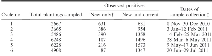
explicitly from data. We calculate risk based on survey data from six cycles of sampling conducted during 2010 and 2011 (see Table 1 for details). In this study example a host location is represented by a single discrete planting of citrus trees. In Florida the plantings are grown in rectangular arrays of regularly spaced trees of varying area (1–205 ha, mean 5.3 ha). Florida contains over 38 000 plantings representing;215 087 ha of citrus (Anonymous 2012b) and they are predominantly situat-ed in the center of the State. The centroid coordinates of each location are known as well as various character-istics such as planting age and size (area).

During each sampling cycle, host locations were selected randomly but with a weighting toward the discovery of a range of important citrus pathogen species including HLB, citrus canker, citrus black spot, citrus leprosis virus, and citrus variegated chlorosis. Weighting for a wide variety of pathogens allows the survey data to be considered approximately random when considering any particular pathogen in isolation. Indeed, the number of pathogens targeted resulted in the deployment of sampling resources over a broad area throughout the commercial citrus growing region in Florida (Fig. 1, Table 1). Up to 15% of the host locations in Florida were inspected during a single round of sampling (Fig.1, Table 1). Each inspection was conducted by a team of trained USDA-APHIS (Animal and Plant Health Inspection Service) plant health inspectors for visible symptoms of a range of diseases, including HLB, and the status of each location was recorded (including either positive or negative for HLB symptoms).

The first component of risk that we need to determine is R0 (Eq. 1). Like many emerging exotic plant

pathogens it is not possible to explicitly calculate R0

for HLB due to a lack of detailed epidemiological data. For HLB the latency and infectious periods of the pathogen have not yet been estimated experimentally (Gottwald 2010). A key determinant of the severity of an HLB epidemic is planting age, with younger trees being more susceptible and infectious (Bassanezi and Bassa-nezi 2008, Gottwald 2010). BassaBassa-nezi and BassaBassa-nezi (2008) show disease progress curves for HLB in citrus plantings of varying ages. By reading data from these

TABLE1. Summary of the survey program for Huanglongbing (HLB) disease in Florida (USA)

commercial citrus plantings.

Cycle no. Total plantings sampled

Observed positives

Dates of sample collectionà

New only  New and current

1 2667 631 631 8 Nov–30 Dec 2010

2 3665 386 954 3 Jan–12 Feb 2011

3 5486 390 1358 14 Feb–25 Mar 2011

4 6248 187 1496 28 Mar–6 May 2011

5 6228 216 1573 9 May–17 Jun 2011

6 4908 87 1347 20 Jun–29 Jul 2011

graphs we estimated the epidemic growth rate, r, for HLB for different tree ages via regression using a logistic growth model.R0 is known to be proportional to the

initial growth of an epidemic as determined by an exponential function of the epidemic growth raterand generation intervalT, i.e.,R0¼exp(rT) (Wallinga and

Lipsitch 2007). Using the Bassanezi and Bassanezi (2008) data we find a linear relationship between R0

and the inverse age of a host location (Fig. 2). We usedT

¼5 as a generation time for HLB; however, the linearity is not significantly different for T ¼ 1 or T ¼ 10. Therefore, we use the inverse age of a host location as proportional to the basic reproductive numberR0 and

thus epidemic size. In addition, planting size obviously will affect R0, and we assume a linear dependence for

this due to a lack of data to quantify more precisely (Keeling and Rohani 2008). Extra hosts intercept the airborne insects or inoculum and subsequently contrib-ute to further transmission. We therefore use the product of the size (S; total area) and inverse age (A) of a host location as proportional toR0, i.e.,R0i}Si/Ai.

The second component of risk is the probability that an epidemic is initiated at locationi,Pi(Eq. 1). For each

host location ithe probability of an HLB epidemic is determined by a negative exponential function of the sum of all Euclidean distances from host location ito

FIG. 1. Maps of Florida (USA) showing the position of Huanglongbing (HLB) sampled plantings for each of the six sampling

positive host location j, i.e., K(a, dij)¼eadij. HLB is

transmitted via a psyllid that disperses repeated short distances and is thus well characterized by the negative exponential (van den Bosch et al. 1999).

Note that this leaves only one parameter value to assign, the exponent of the dispersal kernela. However,

a is not the only parameter in the risk model we have derived for the HLB example. In this case however, we have constructed the model in such a way that, although there are multiple parameters in the model, we only need to assign a value to one parameter,a, since the others can be subsumed into wi by division. However, in

general, for other pathosystems, the number of param-eters that require estimation will depend on how the two components of risk have been constructed for the particular pathogen case. The mean dispersal distance can be calculated from the exponent of the kernelaand can be shown to be 2/a (since we integrate over two-dimensional space) and thus has a clear biological interpretation. The method was tested using the validation approaches described in the previous section

(Model testing). To fit the risk weightings to the data

requires a rescaling of Eq. 1. For the example of HLB we rescale between 0 and 1 by dividing by the maximum risk weighting. This is essentially our rescaling param-eter, which allows us to apply the fitting and validation procedures described earlier.

We separated training and test data in all analyses. That is, specifically, if the method was tested on data from cycleN, the risk estimates were determined using only data from previous cycles not including cycleN. We tested the method accumulatively on different sampling cycles to detect any differences in the accuracy of the method through the course of an epidemic.

RESULTS

Parameter estimation

Here we show results for the two hypothetical scenarios as highlighted in the Introduction: (1) the parameter is known or can be inferred from expert opinion (referred to as the inferred value), and (2) nothing is known and therefore the parameter must be estimated using available data from the survey (referred to as theestimated value). For the inferred value, we use a mean dispersal distance of 10 km for Huanglongbing (HLB). Authors on the current paper have observed and written extensively about HLB, and identified 10 km as a good guestimate of the mean dispersal distance, 2/a, of HLB in the observed region. For the estimated value, i.e., when the parameter is not known, we use the survey data from previous cycles. The estimated mean dispersal distance (2/a) ranged between 3.6 km and 25 km (Fig. 3). A clear minimum in the sum of the absolute errors (SAE) of the risk estimates existed, indicating a strong relationship with positive host locations (Fig. 3). The only exception was in the case of sampling cycle 5 where a minimum SAE could not be found (Fig. 3). This implies that for this cycle the best fit was achieved using the age and size data only, and that the HLB-positive data did not contribute to a better fit (since a zero value foraresults in multiplication by 1) (Fig. 3).

Method testing

As expected, for each SAE-minimizing value, the risk weightings were larger for HLB-positive plantings than for HLB-negative plantings (Fig. 4). The median values of the weightings for HLB-positive plantings were consistently higher than for negative plantings and the distributions were significantly different (Fig. 4). There was little difference between the results for the estimated value of mean dispersal distance, 2/a, (Fig. 4A), and the inferred value (Fig. 4B). The validation based on the receiver operating characteristics (ROC) curves showed good predictive power in each cycle (Fig. 5, Table 2). Cycle 6 was predicted less well due to the comparatively low number of observed positives (Fig. 5, Table 2). The inferred value of 2/aconsistently outperformed that of the estimated value, although the differences were not substantial except in the case of cycle 6 (Fig. 5, Table 2). Finally, the method was also validated in terms of the ability of risk-weighted random sampling to detect new positive host locations via Monte-Carlo simulation (Fig. 6). The performance of risk-weighted sampling using the estimated value closely matched that of the inferred value of 10 km (Fig. 6). However, although the differences between each were marginal for most cycles (Fig. 6: cycles 3–5) the difference was more apparent for cycle 6 (Fig. 6) where the inferred mean dispersal distance of 10 km resulted in a greater performance than the estimated value. However, as previously stated, there were far fewer positives available in this cycle and therefore greater variability in the stochastic sampling

FIG. 2. The change in inverse age of a host location with the

process. As expected, the proportion of observed-positive finds increased with increasing sampling size regardless of the sampling method (estimated-value inferred-value, or simple random sampling) (Fig. 6). The number of finds increased linearly with sample size for simple random sampling but the risk-based sampling plans tended toward an upper asymptote (Fig. 6). The diminishing return of risk-based sampling with increas-ing samplincreas-ing size indicates that a samplincreas-ing size that maximizes the performance per unit of sampling effort can be identified. Further, in practice a particular sampling size that maximizes the gain between random sampling and risk-based sampling can also be identified and potentially used to identify an optimal sampling effort (Fig. 6).

DISCUSSION

In this paper we have presented a generic method to determine risk estimates for an invading plant pathogen in a landscape. This can be used by a regulatory agency to design targeted surveys aimed at reducing inoculum and minimizing further spread. The term ‘‘risk’’ is often used loosely and may be interpreted in a number of varying ways. We adopt a precise definition of risk asthe product of the consequences of an adverse event and the

probability of that event occurring (National Research

Council 2002). In our case this leads to a useful

epidemiological interpretation as the product of (1) the expected epidemic size if the pathogen were to arrive and (2) the probability that the pathogen arrives and causes a local epidemic, P (see Eq. 1). By using a clear epidemiologically motivated definition of risk we pro-vide a transparent and flexible framework that allows available information to be incorporated in a clear mechanistic way based on biologically meaningful processes.

The first objective of a surveying program for an invading plant pathogen is usually early warning— that is, conducting proactive surveillance for a plant patho-gen threat before it has arrived in order to detect it as early as possible following its invasion. We have developed methods to estimate the incidence that an epidemic will have reached when it is first discovered; these methods relate the temporal dynamics of the monitoring program to the dynamics of the invading epidemic, and can be used to inform the design of early warning surveillance programs (Parnell et al. 2012). Some work has also been done to determine spatially optimized monitoring programs to detect an invading plant pathogen at an early stage (Demon et al. 2011). However, once a first detection has occurred the management objective shifts from early warning to one of containment or inoculum reduction. Eradication of plant pathogens is rare due to the challenges associated

FIG. 3. The change in the sum of the absolute errors (SAE), with the mean dispersal distance 2/afor the six sampling cycles:

cycle 2 (minimum ata¼5.53104; mean dispersal distance, 2/a, 3.6 km); cycle 3 (minimum ata¼83105; mean dispersal distance, 2/a, 25 km); cycle 4 (minimum ata¼13104_{; mean dispersal distance, 2/a, 20 km); cycle 5 (minimum ata}

¼0; mean

with, for example, asymptomatic spread and the costs of host removal (Gottwald et al. 2001, Madden and Wheelis 2003, Gottwald and Irey 2007). Therefore inoculum reduction (effectively, damage limitation or containment) is usually the immediate management objective following the first discovery of an invading pathogen. This is especially important if a particular threat was not anticipated and thus no proactive surveillance program was in place to detect at an early stage. Our definition of risk specifically targets this objective since the highest-risk locations are those most likely to carry the greatest inoculum load. The method also maximizes the number of new positive finds since, for plant pathogens, detectable symptoms generally increase with the size of the outbreak (i.e., the first component of risk [Eq. 1]). Epidemiological theory suggests that the earlier mitigation measures are taken the greater the chance of success (Ferguson et al. 2001). There is thus a need for a regulatory agency to respond

quickly to new pathogen invasions, and the risk-based framework provided here aims to facilitate this and provide a rational basis for the design of detection surveys that can be tailored to virtually any biologically relevant plant pathogen.

Our approach is similar to those taken in plant disease mapping, as well as mapping of invasive species more generally. For example, Parnell et al. (2011) demon-strated a method to derive a spatial estimate of pathogen distribution from a random sample; that method captured the limiting effect of spatial pathogen spread that arises from limited dispersal ability and gaps in host availability. Invasive species distribution modelling studies similarly seek to estimate a map of an invader and which can be used to prioritize survey efforts (Allouche et al. 2006, Inglis et al. 2006, Austin 2007, Va´clavik and Meentemeyer 2009, 2012, Williams et al. 2009, Crall et al. 2013). These studies incorporate factors on environmental suitability, presence or absence of the species, and dispersal constraints to arrive at spatially referenced estimates of risk. However, in contrast to these studies, our approach utilizes similar information, but we present a generic and flexible framework in which to do this for plant pathogens.

Additional studies have used population-dynamic models to explicitly link survey and management programs and show how surveys can be further optimized for particular management objectives (Mehta et al. 2007, Cacho et al. 2010, McCarthy et al. 2010, Wallinga et al. 2010, Emry et al. 2011, Giljohann et al. 2011, Homans and Horie 2011, Epanchin-Niell et al. 2012, Horie et al. 2013). For example, McCarthy et al. (2010) showed how, for the control of H5N1 influenza, the optimal distribution of sampling resources depended on what percentage reduction in incidence was attempt-ed. If the reduction was low (5% compared to 10%

incidence) then it was optimal to spread resources more evenly (i.e., the objective could be achieved at less cost by doing this) (McCarthy et al. 2010). Other studies have shown how, for situations where survey and control resources originate from a common resource base, an optimal balance in the deployment of each can be identified (i.e., whether to invest more in survey or control) (Bogich et al. 2008, Hauser and McCarthy 2009, Ndeffo Mbah and Gilligan 2010). Although we do not explicitly link to such management impacts here, a logical development would be to test the method’s performance to determine the optimal use of the risk estimates for different management objectives. For example, if the aim of the management plan is to detect new disease foci (i.e., different disease clusters), then rather than prioritize a survey based on risk alone, it may be optimal to spread survey resources more evenly in space since only one detection per disease cluster would be required. This might be an objective if a two-tiered procedure is in place where a single detection triggers a second stage of localized sampling or a localized host treatment zone. Nonetheless, targeting

FIG. 4. Box plots displaying the distribution of risk

high-risk locations for inoculum reduction or contain-ment is a common managecontain-ment goal and often the immediate objective following a new invasion.

Here we used the economically significant disease of citrus Huanglongbing (HLB) in Florida, USA, as a case study. This disease offers a good test of our method since relatively little is known about the pathogen’s epidemiology, making a spatially resolved prediction of risk challenging. The method clearly out-performed what would be achieved by random sampling (Figs. 5 and 6, Table 2), indicating that even when information is lacking our risk-based approach can significantly improve otherwise entirely ad hoc surveying layouts. Moreover, we have illustrated how the method can accommodate the contrasting scenarios where either some information is known on a pathogen (the parameter values can be inferred from expert opinion) or very little (the parameters must be estimated from available data). We analyzed examples of these scenarios for HLB and did not find significant differences in performance (Figs. 4–6). This indicates the strong role expert knowledge can have when a framework for its inclusion is available. Moreover, where expert opinion can be utilized to parameterize the model much time is saved, thus allowing the targeted surveying program to

be rapidly deployed following the discovery of a new invader.

In the case of HLB in Florida, risk was calculated based on available information, which included the age and size of host locations and their distance to known positives. The two components of risk (Eq. 1) can be calculated in various ways and should be tailored to the pathogen species and information available. The poten-tial local-epidemic size (i.e.,R0) can be calculated either

heuristically, as in the HLB example given in this paper, or using a population model. Which route is chosen will depend on the challenges of calculating R0 for the

FIG. 5. Receiver operating characteristic (ROC) curves for the risk estimates validated based on data from four sampling cycles. The dotted lines denote the no-discrimination line. The solid lines denote risk estimates based on the estimated values of the mean dispersal distance 2/a(see Fig. 3). The dashed lines indicate the risk estimates generated using the inferred valuea¼0.0002 (mean dispersal distance 2/a, 10 km). The closer the lines are to the top left corner (i.e., the farthest from the no-discrimination line) the stronger the predictive power. Note that only cycles 3–6 can be used to validate since two previous cycles are required as training data to generate the risk estimates (in the case of the estimated parameters [solid lines]).

TABLE 2. Area under the receiver operator characteristic

(ROC) curves (AUC) for each survey cycle and the two

compared values of the disease dispersal parameter a,

estimated from the data (estimated a) or inferred from

expert opinion (inferreda), each cycle corresponds to that shown in Fig. 5.

Survey cycle

AUC

Estimateda Inferreda

3 0.656236 0.715305

4 0.580586 0.636254

5 0.70377 0.757957

particular pathosystem. Calculating R0 for HLB is

problematic because of difficulties measuring the latency and infectious periods (Gottwald 2010). In this paper we show how estimates ofR0can be calculated heuristically

and even this relatively coarse approach yields useful estimates of risk (Figs. 5 and 6). More accurate calculations of R0 should lead to more accurate

estimates of risk. For example, Hartemink et al. (2009) demonstrated a model-based approach using the next-generation-matrix method to estimate R0 maps for

vector-borne diseases. Model-based approaches can provide accurate estimates of R0, but at the cost of

extensive information requirements for parameteriza-tion.

The probability that an epidemic occurs,P, can also be calculated in various ways. For example, in the HLB example we used a negative exponential dispersal kernel. Other forms of dispersal kernel such as the power-law could have been used and may be a more appropriate choice for other pathogens, for example if more frequent long-range dispersal events are anticipated. Also the randomized dispersal parametere(Eq. 2) was not used

in our example but could be employed where there are data available. Our method can thus be tailored to suit the differing epidemiological characteristics of a range of pathogen species. Although in the HLB example we have presented it was only necessary to estimate a single parameter in order to fit and validate the model, in other cases there may be more than one parameter and a full sensitivity analysis may be appropriate to understand the risk factors that are having the most influence on the model outcome.

Since detection and diagnostic techniques are imper-fect, and a complete census cannot be collected at each location, imperfect detection may influence the accuracy of the method. A number of studies have shown how likelihood and Bayesian methods can be used to calculate the probability that a location is negative given that a non-detection has been observed and use this to inform estimates of population abundance (Tyre et al. 2003, Mackenzie and Royle 2005, Royle et al. 2005, Guillera-Arroita et al. 2010, Wintle et al. 2012). Hughes et al. (2002), for example, show how for plant pathogens the number of samples required to ensure a

FIG. 6. The relative performance of risk-weighted random sampling with changing sample size (100 Monte Carlo simulations),

site is below a certain incidence threshold can be calculated in the face of misclassification errors and the possibility of non-detection. This is a particular issue with plant pathogens since there is the confounding problem of asymptomatic infection. Although not within the scope of our present study, the accuracy of our validation may of course be influenced by imperfect detection, i.e., that uninfected sites were actually infected. Furthermore, the uncertainties associated with the risk estimates themselves could impact the effective-ness of a survey program. This provides a justification for using a random element to determine a sampling plan (i.e., risk-weighted random sampling) rather than simply ordering locations to survey directly by risk. For example, Baxter and Possingham (2011) suggest that in cases where the underlying risk map is poor, it is more effective to conduct widespread cursory searches than to target resources intensively. Risk-weighted random sampling achieves a similar goal in that where knowl-edge is imperfect sites with low risk estimates still have a chance of being selected. However, if the confidence and uncertainty around the risk estimates are strong for a particular pathogen then a straightforward ranking of locations to survey directly based on risk could be adopted.

The enhanced availability and uptake of epidemio-logically informed methods to determine targeted survey programs is critical in meeting the rising challenges posed by invading plant pathogens. We have developed a generic risk-based method and demonstrated its utility by application to a real problem. We hope our method provides a platform to facilitate the incorporation of epidemiological information into surveying strategies. Indeed the method is used routinely by the USDA Animal and Plant Health Inspection Service to survey for a range of citrus pests and pathogens and has been used by DEFRA to survey forPhytophthora ramorumin England and Wales. The contribution of this paper is to make the method widely available to researchers and policy makers and to test the method on a characteristic plant disease problem.

ACKNOWLEDGMENTS

Rothamsted Research receives support from the U.K. Biotechnology and Biological Sciences Research Council (BBSRC). This work was partly funded by the U.S. Depart-ment of Agriculture Farm Bill and the U.K. DepartDepart-ment for Environment, Food and Rural Affairs (DEFRA). F. van den Bosch received funding from the Bill and Melinda Gates Foundation.

LITERATURECITED

Allouche, O., A. Tsoar, and R. Kadmon. 2006. Assessing the accuracy of species distribution models: prevalence, kappa and the true skill statistic (TSS). Journal of Applied Ecology 43:1223–1232.

Anderson, R. M., and R. M. May. 1986. The invasion, persistence and spread of infectious-diseases within animal and plant communities. Philosophical Transactions of the Royal Society of London B 314:533–570.

Anonymous. 2012a. Britain fights ash dieback. Science 338:586.

Anonymous. 2012b. Commercial citrus inventory preliminary report. USDA National Agricultural Statistics Service. www. nass.usda.gov/Statistics/Florida/ublications/Citrus/citcci.htm Austin, M. 2007. Species distribution models and ecological theory: a critical assessment and some possible new approaches. Ecological Modelling 200:1–19.

Baric, L., M. Zˇupanic, M. Pernek, and D. Diminic. 2012. First records ofChalara fraxineain Croatia—a new agent of ash

dieback (Fraxinus spp.). Journal of Forestry Society of

Croatia 136:461–469.

Bassanezi, R. B., and R. C. Bassanezi. 2008. An approach to model the impact of Huanglongbing on citrus yield. Pages

301–304 in Proceedings of the International Research

Conference on Huanglongbing (Orlando, Florida). Plant Management Network, Saint Paul, Minnesota, USA. Baxter, P. W. J., and H. P. Possingham. 2011. Optimizing

search strategies for invasive pests: learn before you leap. Journal of Applied Ecology 48:86–95.

Bengtsson, V., A. Stenstrom, and C. Finsberg. 2013. The impact of ash dieback on veteran and pollarded trees in Sweden. Quarterly Journal of Forestry 107:27–33.

Bogich, T. L., A. M. Liebhold, and K. Shea. 2008. To sample or eradicate? A cost minimization model for monitoring and managing an invasive species. Journal of Applied Ecology 45:1134–1142.

Brasier, C. M. 2008. The biosecurity threat to the UK and global environment from international trade in plants. Plant Pathology 57:792–808.

Brasier, C. M., S. Denman, A. Brown, and J. Webber. 2004.

Sudden oak death (Phytophthora Ramorum) discovered on

trees in Europe. Mycological Research 108:1108–1110. Cacho, O. J., D. Spring, S. Hester, and R. Mac Nally. 2010.

Allocating surveillance effort in the management of invasive species: A spatially-explicit model. Environmental Modelling and Software 25:444–454.

Chandelier, A., N. Delhaye, and M. Helson. 2011. First report

of the ash dieback pathogen Hymenoscyphus pseudoalbidus

(Anamorph Chalara fraxinea) on Fraxinus excelsior in

Belgium. Plant Disease 95:220.

Crall, A., C. Jarnevich, B. Panke, N. Young, M. Renz, and J. Morisette. 2013. Using habitat suitability models to target invasive plant species surveys. Ecological Applications 23:60–72.

Demon, I., N. J. Cunniffe, B. P. Marchant, C. A. Gilligan, and F. van den Bosch. 2011. Spatial sampling to detect an invasive pathogen outside of an eradication zone. Phytopa-thology 101:725–731.

Diekmann, O., J. A. P. Heesterbeek, and J. A. J. Metz. 1990. On the definition and the computation of the basic reproduction ratio R0 in models for infectious diseases in heterogeneous populations. Journal of Mathematical Biology 28:365–382.

Emry, D. J., H. M. Alexander, and M. K. Tourtellot. 2011. Modelling the local spread of invasive plants: importance of including spatial distribution and detectability in manage-ment plans. Journal of Applied Ecology 48:1391–1400. Epanchin-Niell, R. S., R. G. Haight, L. Berec, J. M. Kean, and

A. M. Liebhold. 2012. Optimal surveillance and eradication of invasive species in heterogeneous landscapes. Ecology Letters 15:803–812.

Ferguson, N., C. Donnelly, and R. Anderson. 2001. Transmis-sion intensity and impact of control policies on the foot and mouth epidemic in Great Britain. Nature 413:542–548. Giljohann, K. M., C. E. Hauser, N. S. G. Williams, and J. L.

Moore. 2011. Optimizing invasive species control across space: willow invasion management in the Australian Alps. Journal of Applied Ecology 48:1286–1294.

Gottwald, T. R., G. Hughes, J. H. Graham, X. Sun, and T. Riley. 2001. The citrus canker epidemic in Florida: the scientific basis of regulatory eradication policy for an invasive species. Phytopathology 91:30–34.

Gottwald, T. R., and M. Irey. 2007. Post-hurricane analysis of citrus canker II: predictive model estimation of disease spread and area potentially impacted by various eradication protocols following catastrophic weather events. Plant Health Progress. http://dx.doi.org/10.1094/PHP-2007-0405-01-RS

Guillera-Arroita, G., M. S. Ridout, and B. J. T. Morgan. 2010. Design of occupancy studies with imperfect detection. Methods in Ecology and Evolution 1:131–139.

Guisan, A., and N. E. Zimmermann. 2000. Predictive habitat distribution models in ecology. Ecological Modelling 135:147–186.

Hartemink, N. A., B. V. Purse, R. Meiswinkel, H. E. Brown, A. de Koeijer, A. R. Elbers, G. J. Boender, D. J. Rogers, and J. A. Heesterbeek. 2009. Mapping the basic reproduction number (R0) for vector-borne diseases: a case study on bluetongue virus. Epidemics 1:153–161.

Hauser, C. E., and M. A. McCarthy. 2009. Streamlining ‘‘search and destroy’’: cost-effective surveillance for invasive species management. Ecology Letters 12:683–692.

Homans, F., and T. Horie. 2011. Optimal detection strategies for an established invasive pest. Ecological Economics 70:1129–1138.

Horie, T., R. G. Haight, F. Homans, and R. C. Venette. 2013. Optimal strategies for the surveillance and control of forest pathogens: a case study with oak wilt. Ecological Economics 86:78–85.

Hughes, G., T. R. Gottwald, and K. Yamamura. 2002. Survey methods for assessment ofCitrus tristezavirus incidence in urban citrus populations. Plant Disease 86:367–372. Husson, C., B. Scala, O. Cael, P. Frey, N. Feau, R. Ioos, and B.

Marcais. 2011. Chalara fraxinea is an invasive pathogen in France. European Journal of Plant Pathology 130:311–324. Inglis, G. J., H. Hurren, J. Oldman, and R. Haskew. 2006.

Using habitat suitability index and particle dispersion models for early detection of marine invaders. Ecological Applica-tions 16:1377–1390.

Jones, D. R., and R. H. A. Baker. 2007. Introductions of non-native plant pathogens into Great Britain, 1970–2004. Plant Pathology 56:891–910.

Keeling, M. J., and P. Rohani. 2008. Modelling infectious diseases in humans and animals. Princeton University Press, Princeton, New Jersey, USA.

Kirkpatrick, S., C. D. Gelatt, and M. P. Vecchi. 1983. Optimization by simulated annealing. Science 220:671–680. Kowalski, T. 2009. Expanse ofChalara fraxineafungus in terms

of ash dieback in Poland. Sylwan 153:668–674.

Mackenzie, D. I., and J. A. Royle. 2005. Designing occupancy studies: general advice and allocating survey effort. Journal of Applied Ecology 42:1105–1114.

Madden, L. V., and M. Wheelis. 2003. The threat of plant pathogens as weapons against U.S. crops. Annual Review of Phytopathology 41:155–176.

McCarthy, M. A., C. J. Thompson, C. Hauser, M. A. Burg-man, H. P. Possingham, M. L. Moir, T. Tiensin, and M. Gilbert. 2010. Resource allocation for efficient environmental management. Ecology Letters 13:1280–1289.

Mehta, S. V., R. G. Haight, F. R. Homans, S. Polasky, and R. C. Venette. 2007. Optimal detection and control strategies for invasive species management. Ecological Economics 61:237–245.

Morgan, B. 1995. Elements of simulation. Chapman and Hall, Boca Raton, Florida, USA.

National Research Council. 2002. Predicting invasions of nonindigenous plants and plant pests. National Academies Press, Washington, D.C., USA.

Ndeffo Mbah, M. L., and C. A. Gilligan. 2010. Balancing detection and eradication for control of epidemics: sudden oak death in mixed-species stands. PLoS ONE 5:e12317. Ovaskainen, O., and I. Hanski. 2001. Spatially structured

metapopulation models: global and local assessment of metapopulation capacity. Theoretical Population Biology 60:281–302.

Parnell, S., T. R. Gottwald, W. R. Gilks, and F. van den Bosch. 2012. Estimating the incidence of an epidemic when it is first discovered and the design of early detection monitoring. Journal of Theoretical Biology 305:30–36.

Parnell, S., T. R. Gottwald, M. S. Irey, W. Luo, and F. van den Bosch. 2011. A stochastic optimization method to estimate the spatial distribution of a pathogen from a sample. Phytopathology 101:1184–1190.

Press, W., S. Teukolsky, W. Vetterling, and B. Flannery. 1992. Numerical recipes in C. The art of scientific computing. Second edition. Cambridge University Press, Cambridge, UK.

Rizzo, D. M., and M. Garbelotto. 2003. Sudden oak death: endangering California and Oregon forest ecosystems. Frontiers in Ecology and the Environment 1:197–204. Royle, J. A., J. D. Nichols, and M. Ke´ry. 2005. Modelling

occurrence and abundance of species when detection is imperfect. Oikos 110:353–359.

Snyman, J. A. 2005. Practical mathematical optimization: an introduction to basic optimization theory and classical and new gradient-based algorithms. Springer, New York, New York, USA.

Timmermann, V., I. Borja, A. M. Hietala, T. Kirisits, and H. Solheim. 2011. Ash dieback: pathogen spread and diurnal patterns of ascospore dispersal, with special emphasis on Norway. EPPO Bulletin 41:14–20.

Tyre, A. J., B. Tenhumberg, S. A. Field, D. Niejalke, K. Parris, and H. P. Possingham. 2003. Improving precision and reducing bias in biological surveys: estimating false-negative error rates. Ecological Applications 13:1790–1801.

Va´clavik, T., and R. K. Meentemeyer. 2009. Invasive species distribution modeling (iSDM): Are absence data and dispersal constraints needed to predict actual distributions? Ecological Modelling 220:3248–3258.

Va´clavik, T., and R. K. Meentemeyer. 2012. Equilibrium or not? Modelling potential distribution of invasive species in different stages of invasion. Diversity and Distributions 18:73–83.

van den Bosch, F., N. McRoberts, F. van den Berg, and L. V. Madden. 2008. The basic reproduction number of plant pathogens: matrix approaches to complex dynamics. Phyto-pathology 98:239–249.

van den Bosch, F., J. Metz, and J. Zadoks. 1999. Pandemics of focal plant disease, a model. Phytopathology 89:495–505. Wallinga, J., and M. Lipsitch. 2007. How generation intervals

shape the relationship between growth rates and reproductive numbers. Proceedings of the Royal Society B 274:599–604. Wallinga, J., M. van Boven, and M. Lipsitch. 2010. Optimizing

infectious disease interventions during an emerging epidemic. Proceedings of the National Academy of Sciences USA 107:923–928.

Williams, J. N., C. W. Seo, J. Thorne, J. K. Nelson, S. Erwin, J. M. O’Brien, and M. W. Schwartz. 2009. Using species distribution models to predict new occurrences for rare plants. Diversity and Distributions 15:565–576.