The Heat Transfer Coefficient as a Function of Steam Quality for High Pressure Once Through Flow Boiling, with Determination of the Transition Points Between the Regions of Particular Heat Transfer EUR 4561

(1)

>*»iÆ3i;

U R 4 5 6 1 e

m

THE HEAT TRANSFER COEFFICIENT

AS A FUNCTION OF STEAM QUALITY

FOR HIGH-PRESSURE ONCE THROUGH FLOW BOILING,

WITH DETERMINATION OF THE TRANSITION POINTS

BETWEEN THE REGIONS OF PARTICULAR HEAT TRANSFER

. .ii*W I.J

if

mi

m

L. NOBEL

MKKPBÍ

(2)

LEGAL NOTICE

Γ'»^J^M»",4^··'*'t",

mi'

'm

wwMåmmm

mNmmêimmt

This document was prepared under the sponsorship of the Commission of the European Communities.

Neither the Commission of the European Communities, its contractor;

l ' í . V t . t í

nor any person acting on their behalf :

make any warranty or representation, express or implied, with respect to the accuracy, completeness, or usefulness of the information con tained in this document, or that the use of any information, apparatus, method, or process disclosed in this document may not infringe VW™

I

PH*'δίΑΜίτΤ' origins«'afta MlTrøEff JicStf? J1 Ώ 8 ^ -'h'*'Ψ&ν

This report is on sale at the addresses listed on cover page 4

at the price of F F 11.— Β. Fr. 100.— DM 7.30 It. Lire 1,250 Fl. 7.25

When ordering, please quote the EUR number and the title, which are indicated on the cover of each report.

**1*ΐ$»**

illiillÉi

Printed by Guyot, s.a., Brussels

»ftp

mm

Luxembourg, November 1970

m

(3)

EUR 4561 e

THE HEAT TRANSFER COEFFICIENT AS A FUNCTION OF STEAM QUALITY FOR HIGH-PRESSURE ONCE THROUGH FLOW BOILING WITH DETERMINATION OF THE TRANSITION POINTS BETWEEN THE REGIONS OF PARTICULAR HEAT TRANSFER, by L. NOBEL Commission of the European Communities

Joint' Nuclear Research Center - Ispra Establishment (Italy) Engineering Department - Heat Transfer Division

Luxembourg, November 1970 - 70 Pages - 28 Figures - B. Fr. 100.—

In a "once through" process in which water at a temperature far below the saturation temperature enters the tube, and leaves it as superheated steam, the heat transfer takes place according to different mechanisms each of which is active over a limited length of the tube.

As far as the present state of knowledge permits, the heat transfer coefficient for a particular heat transfer region is determined analytically as a function of the mathematical steam quality X, for different heat and mass fluxes and pressures between 170 and 210 bar.

ι

I

EUR 4561 e

Joint Nuclear Research Center - Ispra Establishment (Italy) Engineering Department - Heat Transfer Division

EUR 4561 e

Joint Nuclear Research Center - Ispra Establishment (Italy) Engineering Department - Heat Transfer Division

In a "once through" process in which water at a temperature far below the saturation temperature enters the tube, and leaves it as superheated steam, the heat transfer takes place according to different mechan;sms each of which

is active over a limited length of the tube.

(4)

Also, for X values indicating the transition between the different regions of heat transfer, equations have been set up as functions of the same parameters. The theoretical background of these equations differs in some cases from the actual theories.

Maybe one of the most unconventional approaches to the problem is the assumption that the pipe length over which film boiling takes place can be determined by using an analogy with a water-jet-gas-pump aggregate.

This method indeed seems to give a useful correlation equation.

(5)

E U R 4 5 6 1 e

COMMISSION OF THE EUROPEAN COMMUNITIES

THE HEAT TRANSFER COEFFICIENT

AS A FUNCTION OF STEAM QUALITY

FOR HIGH-PRESSURE ONCE THROUGH FLOW BOILING,

WITH DETERMINATION OF THE TRANSITION POINTS

BETWEEN THE REGIONS OF PARTICULAR HEAT TRANSFER

by

L. NOBEL

1970

Joint Nuclear Research Center Ispra Establishment - Italy

(6)

A B S T R A C T

KEYWORDS

HEAT TRANSFER TUBES MATHEMATICS BOILING STEAM FILMS FLUID FLOW PUMPS

(7)

C O N T E N T S

1. INTRODUCTION 5 2. THE HEAT TRANSFER-COEFFICIENT-STEAM-QUALITY CURVE 9

2.1. The liquid phase forced convection heat transfer

coefficient as a function of thermodynamic quality 1C 2.2. Calculation of the X- value at which

subcooled boiling begins '5 2.3. Calculation of the subcooled boiling heat transfer

coefficient 15 2.4· Calculation of the saturation boiling heat transfer

coefficient 1 8 2.5· Determination of the X- value at which the heat

transfer-crisis occurs 20 2.6. Determination of the X— value at which the ultra

crisis region starts 25 2.7· The relation between heat flux, wall temperature

and mass-flux 29 2.8. Determination of the heat transfer coefficient in

the transition and ultra crisis regions 30 2.9. Approximata construction of the X- value at which

the ultra crisis region ends 32 2.10 The maximum heat transfer coefficient in the ultra

crisis region 33 2.11 The heat transfer coefficient in the region of vapor

phase forced convection heat transfer 3h.

3. CONCLUSION 35

TABLES 38 - '+6

KEY TO THE FIGURES ^7

FIGURES ^9 - 63

NOMENCLATURE Sk

(8)

(9)

1. INTRODUCTION *)

If the oooling of a heated channel is performed by flow boiling of water at a pressure lying in the near subcriticai range (17O - 210 bar), relatively high heat fluxes may be applied

without causing excursions of wall temperature severe enough to damage the material of the wall.

Normally a certain amount of heat transfer deterioration will

ooour, but the maximum temperature to be attained by the wall can be predicted knowing such parameters as mass flux of the coolant, pressure, diameter of the ohannel and heat flux to be

supplied. If the operating limits, determined by the material of the wall, are taken into account the whole scale of heat transfer modes can infact be subsequently realised in a heated ohannel,

beginning at the entrance of the ohannel with forced oonvection heat transfer in the sub-saturation temperature range and terminat-ing with heat transfer in the superheated vapour region leavterminat-ing

the channel.

As soon as the wall temperature slightly exceeds the saturation temperature of the liquid, nucleation starts and the subcooled boiling becomes the main type of heat transfer. After the hulk temperature of the liquid has reached saturation temperature, fully developed boiling takes place, hut thie merely depends on the magnitude of the difference between wall temperature and satu-ration temperature. Given the fact that onoe boiling has begun, the wall temperature soon raaohes a level that remains constant over the whole nuoleate boiling region, one may say that fully developed boiling normally starts already far in the suboooled boiling region.

(10)

As we know from the current literature, the breakdown of

nucleate flow boiling follows the onset of boundary layer

separation.

It can be imagined that the onset of boundary layer separation

should be a function of the channel length over which fully

developed nucleate flow boiling occurs} the mass flux, the heat flux, the channel diameter and the pressure of the system.

The breakdown of nucleate boiling causes the formation of a vapour layer stratified over the wall, giving a steep increase

in wall temperature. The core flow surrounded by the vapour layer now acts as a kind of jet, and the system jet vapour layer simulates to a certain extent a water jet gas pump aggre-gate.

A very-well-known phenomenon of liquid jets is the discontinuous enlargement of the jet which refills the entire oross seotion

of the duct. This behaviour can also be expected at a oertain distance down-stream from the breakdown point, resulting in restabilisation and re-configuration of the flow-pattern, due

to the intensive mixing of the phases. This «stabilisation point coincides with the point of maximum wall temperature, although this latter point oan have a certain extension of length.

This is due to the faot that although the wall cooling is

improv-ed, it continues to be governed by a process of quenching of the hot wall. The high wall temperature impedes rewetting and re-nucleation and the system behaves as a peripherically flashing

(11)

7

-The heat transfer in this ultra orisis region depends mainly upon the gas phase characteristics, although the influence of

droplet deposition strengthens dependency on the mass flow

rate.

Up to a certain steam quality, the heat transfer improves steadily due to an increase in the two phase velocity and the

spray effect of droplets on the wall.

Beyond this steam quality a thermal disequilibrium is established between the vapour phase near the wall, and the liquid phase

moving in the oentre part of the tube. The vapour annulus at the

wall becomes more and more superheated, whereas the oore, consist-ing of a mixture of vapour and water droplets, remains at

satura-tion temperature.

The heat transfer from the wall to the superheated vapour annulus occurs aooording to the laws for superheated steam so that the wall temperature will gradually increase again, and the heat

transfer coefficient will decrease. Up to now we have given a brief description of the heat transfer phenomena occurring in a once through flow boiling system at high working pressures.

(12)

At moderate heat fluxes the crisis starts in the annular dispersed flow regime and heat transfer deterioration oocurs through the

drying-out of the fine water film on the wall. Initially this introduces a steep increase in wall temperature due to contact between the vapour and the wall. Further wall temperature increase

depends on the steam quality. For the lower qualities the tempe-rature will decrease once more, but for the higher qualities the temperature will continue to increase because the fluid behaves .

like superheated steam.

It will be clear that in this case no particular jet aotion can

exist and the heat transfer minimum depends only on the heat exchange between the superheated vapour flowing in the vicinity of the wall and the liquid droplets moving in the oore. (For

further information see the work of BENNETT et al. J_ 1_/) .

Although, as we have mentioned already, no oomplete simularity oan exist between the types of heat transfer to be expected when

the critical heat transfer conditions are fulfilled under differ-ing circumstances in different parts of the system, there are nevertheless certain common features to remark. In the region

upstream from the crisis the wall is wetted and the flow regimes are in accordance with the model given by COLLIER ¡_ 2_/.

In the region downstream from the crisis the wall is not wetted

and the flow regimes differ from the model given by COLLIER and

(13)

As we have discussed in the foregoing paragraphs,the heat transfer in

a once through flow boiling system whirJh inoludas preheating of

the water and superheating of the steam, is a polyform phenome

non with a number of caraotheristic transition points and

distinct heat transfer regions between them.

Although f rom a strictly heat transfer point of view, the

maximum allowable wall temperature is the only restricting

parameter and all other wall temperatures beneath this one

are of seoondary importance, in this work a oomplete summing

up of the equations governing the heat transfer in the differ

ent regions will be given as well as the equations or diagrams

predicting the transition points between these regions.

All equations are written as far as possible as functions of

the steam quality x, being the ratio between the increment of

enthalpie over the saturated liquid state and the latent heat

of evaporation. In the case of subcooled heat transfer χ is

negative. The data used are taken from the work of HERKENRATH

and MORKMÖRKENSTEIN ¿ l j .

2. THE HEAT TRANSFER COEFFICIENT STEAM QUALITY CURVE

General outline of the curve.

Fig. 1 reproduoe« a curve oC versus χ taken from J_ 3_/·

This figure shows the typical heat transfer regions as well

as the transition points labeled with the figures 1 up to and

(14)

-

10

1) Region in which heat transfer to the liquid phase is performed by forced convection

2) The X—value at which subcooled boiling starts

3) Region of suboooled boiling heat transfer 4) Region of saturation boiling heat transfer

5) The X—value at which the heat transfer orisi s occurs

6) The X-value at which the ultra crisis region starts 7) The minimum value of heat transfer coefficient

8) The region of transition and ultra crisis heat transfer 9) The X-value at which the ultra ori si s region ends

10) The maximum heat transfer coefficient i$ the ultra ori si s region

11) The region of vapour phase forced convection heat transfer.

The area between 2 and 5 is approximately the area in which

fully developed boiling exists. The region of vapour phase forced convection heat transfer can belonglpstrtiàlly to the wet vapour region and partially to the superheated steam region.

The reproduction of ct in the transition between region 1 and

3 has to be approximated beoause systematio measurements to calculate this transition are not available. In the following pages the mentioned points from 1 to 11 will be discussed more

profoundly and equations to calculate the magnitudes pertinent to the matter in question will be derived.

2.1. The liquid phase forced oonvection heat transfer coefficient

as a function of thermodynamic quality

(15)

11 In such cases it would be wrong to use bulk temperature only

as the reference temperature for the calculation of the charac

teristic physical constants, as is frequently done e.g. as in

the PETHUKOV equation

J_ ¿±_]

reproduced here below:

* P

q.

σ

„

H

m pB

8(1,82 lg Re 1,64)

2

Í 1,07+1 2,7\/

~

B L

V

8

(l,82 1g

lg Re

B

1,64)

(Pr|

/3

l)j

(11)

For the supercritical region HERKENRATH /

$_/

modified the

PETHUKOV equation introducing the wall PRANDTL number and the

influence of the heat capacity taken at the wall temperature.

His formula:

0Í

Η

q

C

*m

pW

8(1,82 lg Re 1 , 64)

2

i 1,07+1 2,7\/

1

B

l

V 80,82 1g

Re

B

1,64)

(12)

gives good results in the case Pr„^Pr^.

W B

For c i r c u m s t a n c e s u n d e r which Pr S Pr , the o r i g i n a l PETHUKOV

ft SJ

(16)

12

range (170210 bar), the PRA.NDTL number goes through a minimum

at an average value of about 260 degrees C. This means that

for Τ > 260 deg. C the PETHUKOV equation can be used and for B

T < 260 degrees C the HERKENRATH equation. B

This temperature is only a rough indication however.

By using a "mixed equation", we found that:

q λ / Ο C

\ V pff pB

\ 1,07+12,7^

1

'80,1

8 ( 1 , 8 2 l g Re 1 , 6 4 )2

■D » —r/ ι ■ ι " > · ■ —ï ' y ρ

' 82 l g Re 1 , 6 4 )

B

^

* ;

/ 3

-

D}

(1-3)

The transition point between the PETHUKHOV equation and the

HERKENRATH equation can be found more easily if the following

condition is fulfilled:

A y (equation 1—2) » 0\^.(equation 13)

Moreover it seems that the "mixed equation" especially for the

higher heat fluxes gives better agreement in the region above 260

degrees C .than the other two methods. Unfortunately the experi

mental information at our disposal is toofragmentary for

a definite conclusion to be drawn.

Remark:

The method of o a l o u l a t i n g 0( i s the following:

F i r s t s t e p :

T

J51 ff Now i s T » T q / / V

B2 ff V OCf C a l c u l a t e 0( a s s u m i n g T

(17)

13

Second s t e p :

C a l c u l a t e ot using Τ

2 B¿

Now is Τ » Τ q. /oc B3 ff V ^ 2

The number of steps is determined and limited by the condition

that T Τ , ^ 0,001 Τ

Bn Bn+1 Bn

A temperature interval for Τ of 10 deg. C is normally sufficient.

w

The c a l c u l a t i o n of 0C follows from T

Bn+1

The bulk temperature gives also the enthalpie decrement A h sat

to be taken from the steamtable in order to calculate x, accord

ing to the formula

x T ^ ( 14)

From the foregoing it will be clear that functions of OC explicit

in χ are not to be expected for the moment due to the lack of

sufficient information. However the method desoribed so far gives

the indirect relation between the two functions.

In Table 1 we have given some examples of the calculation of T B using equations (1i) (12) and (1—3)· In a fourth column the measured values of T so far determined are also indioated.

B

2.2. Calculation of the Xvalue at which subcooled

boiling begins

As we have disoussed already, the wall temperature increases

until a constant temperature level has been reached lying

slightly above the saturation temperature. In 3 we will develop

(18)

14 oase of boiling.

In the context of the actual problem

w

hich is to calculate the Xvalue

at whioh subcooled boiling starts, we may assume with a good

approximation that boiling starts as soon as the wall tempera

ture has reached the saturation value. In the subcooled region

'the general expression for X may be constituted also as:

X « (T Τ ) C

κ Β

S

;

ρ

(21)

From whioh:

τ τ /

S Β J

Using t h e PETHUKHOV e q u a t i o n we o b t a i n f o r Τ Τ t h e e x p r e s W o

s i o n :

4,

1,07+ 12,7 V ? / 8

( P r

2 / 3

i ;

- ')

^-\'7^Z

=

(2

-

3)

Hm pB

w i t h

5/8

2

( &

"

3 a )

8 ( 1 , 8 2 l g ReB 1,64)

S u b s t i t u t i n g Τ — Τ i n ( 2 1 ) by t h e e x p r e s s i o n a c c o r d i n g t o B S

(2—3), we o b t a i n f o r t h e X—value a t which n u c l e a t i o n s t a r t s :

i.

.

c

11,07+12,7 V V e Í P r !

/ 3

OJ

(19)

15

This equation may be substituted by a simpler one, assuming

that the numerioal value of the expression

pB

| l , 0 7 + 12,7

V V M P X B

2 / 3

-

D ]

will lie between narrow, limits.

Assuming that this is the case, and remembering that ΗΘ Si Re0,

B S the formula (2-4) becomes then,

\ 2

\ ' - C v η τ (1,82 lg Re - 1,64) (2-5)

Ν Ν q · L S m

Here Cjj is a coefficient to be determinedby the experimental da ta. From our data we have deduced the following values for C Ν

Ρ - 170 bar C - 10,963

Ν

Ρ =· 185 bar C

>T

- 11,343

Ν

Ρ - 195 bar C - 11,669

Ν

Ρ - 205 bar C - 13,103

Ν

Ρ - 210 bar C « 13,914

Ν

These values of C give calculated X - values lying between the

+_ 10 % error l i m i t s of the experimental X - v a l u e s .

2.3· Calculation of the subcooled b o i l i n g heat t r a n s f e r c o e f f i c i e n t

From the method described in 1, we have oaloulated up to the

" q u a l i t y " X the forced oonveotion heat t r a n s f e r c o e f f i c i e n t s .

This means that the value Ci

w

corresponding to X„ i s a l s o

known. From that point we enter a t r a n s i t i o n region in which

surfaoe b o i l i n g w i l l be e s t a b l i s h e d .

(20)

16 at which nucleate boiling will be fully developed and the wall

temperature remains constant for the smaller q, values far up

h

into the positive X range untili the heat transfer crisis starts.

The temperature difference in the subcooled boiling region may

now be found from:

Δ Τ Δ Τ

+ Δ Τ

(see Fig. 2)

sub

f

Δ Τ , may be found from equation ( 2 l ) , g i v i n g

sub

Δτ ,

4 ^

Í

3

"

1

)

sub

C

Ρ

When looking for an expression for Δ Τ , we may conclude that

the passion of "boiling" experimentalists for describing the

relation between boiling magnitudes in the form Nu =

φ

(Re, Pr),

is nearly ineradicable. So we will also try to find a useful

equation in the same way. The general equation for flow boiling

would then be:

Nu C . Re

y

. Pr

Z

(32)

This equation implies t h a t OCis anindependent function of q, .

h

S p e c i f i c a t i o n and rearrangement of t h i s equation g i v e s :

„*, 1y ..

., ï»

A m L qh

Δ τ

\

Η hfl <»)

f

C' C^ L q

p f

*m

In the REYNOLDS number of this equation, a length parameter

ψ

indicated by D has been assumed, whose magnitude depends normally

on pressure and tube diameter. For pool boiling (q 0, q > 0),

m

h

similar formulae are ohoosen, to be expressed in the most general

(21)

17 Δ τ

t/L

· i V

C' C

Ρ o

1^1 l=£

/ * '

m

O M )

Also,in this equation 1

may depend on system dimensions and

physical constants, often 1 is a function of bubble diameter.

A mean value for η would be η ■ l/3, and according to ROSENOff

¡_

6__/ is for water at high pressures m « 1 . Applying these

values and combining the two equations we obtain the result:

o

, 1 y

« 1 / 3

Δ τ Δ τ

— D

1 f

o 0

f

C ' 1Λ'

L λ '

- z

2/3 f

L *_mm ra

2/3-y

(3-5)

From their subcooled boiling experiments ZENKEVICH and SUBBOTIN

2 m

Assuming that this dependency will be sustained to some extent

¡_ 1_]

obtained the relation q © c q

m

· into the positive quality region, we obtain as a universal value

for y; y «

ΐ/3· As long as ζ remains an unknown exponent,

the expression

* -·

■"

Ί¥Γ

will be substituted by the new parameter 5

_{. By doing this}

τ

we arrive at the temperature equation for saturated flow boiling

i .Θ?

A?. - Δ τ

f o

,-

q

h

2

α

Γ

Ì1/3

V

¿

T

/——/

/ ——

-ι

m

'

For p o o l b o i l i n g v e f e u n d Τ « Κ / » q

So we o b t a i n f o r e q u a t i o n ( 3 6 )

1/3

(22)

18

2 1/3

Í lv,

q

*

6Φ

1 (37)

Writing for

equation (37) may be written as

m

The function'M/ f(p) has been plotted in Fig. 3· It is a

unique function of the pressure. Combination of the equations

(31) and (39) gives the temperature difference in subcooled

boiling

Δ Τ

' Ρ

+

^ T V 3

<^°>

ρ

m

The heat transfer coefficient is now to be found from

** subcooled

77E

V f · *h

(311)

C ~

+

1/3

P \

2.4· Calculation of the saturation boiling heat transfer

coefficient

The difference between wall temperature and saturation temperature

may be calculated by equation (39)· This formula leads to a

very simple expression for the heat transfer coefficient in the

(23)

19

0,33

<?C - -A- = - f -

(4-1)

2 Keeping i n mind t h a t under s i m i l a r c o n d i t i o n s q, oC q , we

h

m

may state that also for inoipience of boiling α

» k . q ,

ni

i

m

inserting this relation in equation (41)> we obtain for the

heat transfer ooeffioient at boiling incipiency :

q

°>

6 6

oí

-

-ΤΤΓΤ

(4

-2)

κ

Ο,33 γ

i

' f

DAVIS and ANDERSON

[_ 8_/

proposed the following relation for

the wall temperature difference at boiling incipiency :

_ 8 G τ

_ 0,5

n

_

Δ Τ /

S /

q

0

'

5

(4_3)

giving for the heat transfer coefficient

■ λ L p " "

7

The difference in exponent between the equations (42) and

(44) may be explained by the difference in type of boiling.

The formuîmof DAVIS and ANDERSON has to be applied mainly for

annular flow conditions»w.hich seems to be confirmed by the work

of K0PCHIK0V et al.

¿

9_/ who found roughly the same relation as

(43) for liquid film pool boiling i.e.

G T

_0,5

0

ς

(24)

20

However in 5 it will be seen that the work of MORKMORKENSTEIN

and HERKENRATH / l j is restricted mainly to the bubbly

flow regime.

2.5· Determination of the X value at which the heat transfer

crisis occurs

On the threshold of the heat transfer crisis, equation (36)

may be used to calculate the dimensionless temperature dif

ference:

Z>

Tf

3 q^

2 q

m

· S

T

o m '

The right hand side of equation (5—1) may also be used as a

correlating group for the determination of the steam quality

at which the wall temperature almost stepwise starts to

rise. Such correlating groups are already described in the

literature. The correlation of TONG / 10_/should be transferred

intothe equation:

L^J

L-^T-J

. * ♦ « £

(52)

m '

Our group correlates in the following manner:

¿rrW

L-^J

-\«-\

(5-3)

m '

The function υ can be taken from Fig. 4ι and is a unique

(25)

21

The c o n s t a n t χ i s a weak f u n c t i o n of t h e p r e s s u r e i n t h e r e f

p r e s s u r e r a n g e : 170 ^ Ρ ¿ 210 b a r .

The v a l u e s a r e g i v e n i n T a b l e 2 .

P ( b a r ) 170 185 195 205 210

X

ref

° '

4 1

° '

4 2

° '

4 2 5

° '

4 3 5

°

> 4 4

The i n t r o d u c t i o n of a r e f e r e n c e v a l u e χ _ i s a l s o known i n

ref

the heat transfer literature. The correlation of C.I.S.E.

J_ 11_/ takes the form:

η A P °»4

- \ - \'

^°

, 4

(-f-D

I-.P/P„

ZrfV

E

^ x

(54)

L q

m

0,794

(W

C

MOOO'

I t i s c l e a r from t h i s e q u a t i o n t h a t :

1 P / P

Xr e f » q 1/3 ( 5 5 )

M000y

I n our r e s u l t s we c o u l d a l s o o b s e r v e a weak dependence of χ

ref on q . ffe have nevertheless ignored this influence in our correla

lo

tion. The question now arises as to whether the correlation so

far developed is a so called overall correlation or is it oonneoted

to a specifio flow pattern? In order to answer this question, we would first like to demonstrate the subtlety of the problem. For

Ρ 170 bar ι

data groups:

2

(26)

\

m

SS

9 2 , 5

102,44 123,94 146,32 X X X X 10* 104 104 104

, 2 ff/m

22

-X 0,354 c

X - 0,338

o

X 0 , 3 0 2 c

X - 0,273

c

P l o t t i n g t h e s e f o u r g r o u p s r e s p e c t i v e l y i n a / / X

- <lv - L Q-m °

Ζ

η "τ m

—_/— X d i a g r a m , we o b t a i n t h e c u r v e s

m

printed in Fig. 5· Three data points correlate proportionally Ih

better with ~ , and two points presumably correlate with

,*h 72 L , tm

/ I . The transition between the two regimes is situated L.q

at a A— value of 0,3» corresponding to a volumetric quality

A of 0,68. Note

X V" + ( ix)~^r

X V

ß '

τ

V" +

(

ixì ir*

Due to the very low slip between the gas and liquid phases

at the high working pressures, we can state that the void

fraction is nearly equal to the volumetric quality, certainly

in the bubbly flow and mist flow regimes. A void fraction of

0,68 may correspond to the transition region from bubbly flow

to annular flow. In Fig. 6 we have plotted all the data points

of X in a V" — V' diagram,

o A A

V" « q . Χ . v" (the "superiioial" steam velocity)

A m

V* « q . (1X) r* (the "superficial" water velocity)

A m

In thi β diagram ƒ?> «- lines are linear functions going through

the origin. Assuming that OC and β are identioal, it follows from the diagram, that for 78^ of the data point· the

(27)

23

In Fig. 7 we have reproduced a group of 19 data points from

LEE /~12_7, with

q « 4134 + 3 , 3 $ a t + 71 isg/om

m — —

The points for X <. 0,09 correlate proportionally with

2 °

/ q^/L q 7 and the points for X > 0,09 with / q^/L q _/.

h m c ' h m

For Χ ■ 0,09 i s ft « 0 , 6 6 . From the foregoing i t can be

concluded t h a t f o r the bubbly flow regime the b u r n o u t or heat

t r a n s f e r d e t e r i o r a t i o n q u a l i t i e s c o r r e l a t e with a high p r o b a b i l i

t y according to a formula of the form:

**X * - X**

- Ζ ~ Ά -

J

2 R

e l (5-6)

r e f c *- L.q -J eq w /

m

for high pressures Ρ ^ 170 bar is m « 1. It further follows that

a small part of our data will presumably correlate better propor tionally with q / L q . This means that to a certain extent our

h m . -correlation is really an overall -correlation. However, this mainly bears upon the choice of the value for X .. From Fig. 5

ref

it can be seen that our X _ - values are between X „ „ ■ 0,38

ref ref B

and Χ „ 0,505. Note: ref A

χ _ _ i s X „ value for the bubblyflow regime ref B ref

Χ is Χ _ value for the annularflow regime, ref A ref

It will be clear that overall correlations are blurring out

the typical characteristics of a burnout curve. However with

some imagination an overall correlation can be redivided into

two branches, one of which corresponds to the form of equation

(28)

24

As an example we have written the correlation of MIROPOLSKII

SHITSMAN [_ 13_/ in our notation. It becomes:

_ <L _ 2 _ q . £ m

(l-zf-ÍT^J

L-J^J

(57)

m / ,

\ Λ

Γ Ρ

1

-f>,2^ ,

-2

In t h i s formula m 1,2 and f o r

—

Lp^J

/> 6.10

i s η ■ 6. In the e q u i v a l e n t Reynolds group

ζ

i s the following

A.

f u n c t i o n :

2 h

—τ-

^)

2 (cV)

1 , 3 3

(r/f)

0 , 1 3 3

(ïï)

1 '

6 6

Ρ »

(58)

f o r l/D /MOO i s

C » 0,174.

Plotting / q, /L q / . Re versus (1X ) , we obtain a curve

* ^h ^m—' v o

as has been shown in Fig. 8. For X ^ 0,10 the ourve may be c

approximated by a straight line indicating the relation

m

For X the value 0,20 will give the best resul*.The part between ref

X « 0 , 1 0 and X « 0,40 may be approximated very well by a

c c

function of the form

X

L-T^—J

· Re°'

6

(510)

ref o * L. q —' v '

Here Χ Λ « 0,52. ref

Except for the rudimentarilyexisting annular flow branoh of the

burnout curve, a third branoh may be blurred out by the form

(29)

25

already by DOROSHCHUK / M^_J to be covered by the steep

decreasing part of our correlation approaching X „. Burnout

r e t

a t t h i s branch i s c h a r a c t e r i s e d by dryingout of the water

film on the w a l l . The X value a t which t h i s phenomenon occurs

can be c a l c u l a t e d by means of a r e l a t i o n given by HEffITT and

PULLING / ~ 1 5 _ / . Writing the l i m i t i n g X value in f u l l we o b t a i n :

xti

χ

1L I ( i î = 5 ) dx

q m E a

(1 X )

(511)

L l

'

d Z

\

SnEa

7 T . D q

h

In this equation q _ is the entrained mass flux at the point

mEa

f o r X » X where annular flow s t a r t s . According t o DOROSHCHUK

a

X,. i s a constant value f o r a whole range of q v a l u e s . HEWITT

l i

h

and PULLING however have given several arguments to explain that

for smaller q values (and thus increasing boilinglengths)

dq _/dz, q _ and X take different magnitudes from those at mEr mEa a

higher q values. Acoording to this fact,therefore,X may be

h li

expected to increase slightly with decreasing q, . The discussion h

so far will have made clear that the correlation given by equation

(53)> theoretically holds only for the suboooled boiling and

bubblyflow regime. However by the o o r r e c t choice of X _, the

ref

oritical parameters in the liquidfilm boiling regime and in

the liquid deficiency regime oan also be predicted. An illustra

tion of this principle is given in Fig. 9·

In Table 3 a synopsis has been given of the experimental r e s u l t s

(30)

- 26

between experimental results of X and the calculated X - values,

c c for D - 10 mm and for D » 20 mm. The maximum deviation between

X measured and X calculated amounts to about X - + 0,05· The

c c — influence of D is in the range of investigation very weak and

thus may be ignored. The range of validity of the correlation

lies between X - - 0,1 and X _ *= 0,44· _{c ref max}

2.6. Determination of the X- value at which the ultra crisis

region starts

General considerations

At the point of heat transfer crisis, the liquid separates

from the wall and a steam layer is formed, under which influence the wall temperature increases as a function of length. In the case of bubbly flow the volumetric content of the liquid in the bulk stream amounts to more than 32%. This enables the bulk

(31)

27

onset of an amelioration of heat transfer coincides with a

reorientation of the fluid flow.

Calculation of X ^ . .

Ifweconsider the momentum exchange in the mixing cross section,

(see Fig. 11) the summant of core mass flux and film mass flux

is equal to the mass flux q thus: m

K + «U 9 . (61)

k f m

Further is q „ * q (Χ, Χ ) (62)

*f *mv *min c' '

From equations (6I) and (62; follows, that

IT,

» q. Ζ 1 -

(

x

øC

· -

x

)_7

(63)

k m * "Snm c

Introducing the mass flux ratio

qf

m » —

\

it follows from equations (62 to 64) that

xv . χ

** m m c m «

(64)

1 (Χ, . χ )

ν * m m c

(65)

The momentum exchange can be calculated from the momentum

balance, Momentum loss ■* Momentum core flow + Momentum film

flow Momentum after mixing cross section.

Momentum core flow *

L

1 (ΧΛ/ . X ) _ /

L

0

x

oC · ) V' +

X V"_y q

2

/f (oc>)

* »min c —' ·* Λϋΐιη c —' m ' x '

(32)

28

Momentum f i l m flow »

(

χ

*

· -

χ

) r - 7

α!

ί

6

-

8

)

^•min c 1 - f m

Momentum a f t e r mixing c r o s s - s e c t i o n «*

H

1_X ) ΛΓ' +

x

Ä

V " V q.

(6-9)

^ iliDin' * m i n ' m v '

Because the momentum loss is partially transferred into a

pressure recovery, the maximal attainable pressure recovery

ratio is:

_. momentum loss

ι Ι ! _{m a x} _{m o m e n t u m b e f o r e m i x i n g c r o s s s e c t i o n}

or

( XA , X )2 V " / l f / ( 1 X , )V» + x . V"_y

n

^ m i n c/ ' ^ * m m ' *min -1 , , ,„» m 1 + _ _ _ _ _ ( 6 1 0 )

h

- ( χ * · -χ V

L

χ ν- + ( ι +

Xoc

. )vvi/f

*" Λυ ι η c^ ^ c Λπ ι ι η —'

Assuming t h a t we may s u b s t i t u t e :

X V" + (1 X . )V« by ¿(t X . . )V' + X ^ . V"J ξ c "mm * v am i n et mi η

w i t h S * c o n s t a n t o v e r a s m a l l m r a n g e , b y i n t r o d u c i n g

m.we o b t a i n :

ry

m 1 +

f :

m

2

· V"

_ (m+l).f

SOf)'(m+l) /"X^ V»

+0X . )T'J

I

otmin ^rnin —'

The p r e s s u r e r e c o v e r y a s a f u n c t i o n of m w i l l b e a m a x i m u m f o r

max dm

T h i s i s

0 .

(33)

29

"I

Xe«. v" + O X w )v'

c " # min ' 1/ ν · ■/ 'V"

/ / v —'min Äm i n / , , N

χ χ _ 1 + 1 / 1 _ ( i _ f ) — ( 6 1 1 ) c # m m 1/ v ' f

T h i s f o r m u l a w i l l be u s e d a s a p o t e n t i a l c o r r e l a t i o n e q u a t i o n

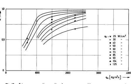
between X and X J . I n F i g . 12 we have p l o t t e d t h e f u n c t i o n c c*· min

f v e r s u s ¿ X * X » X .

Λ mm c

For pressures in the range 170^ Ρ ¿210 bar, a single curve

may be used. Fig. 12, 14> 15> 16 and 17 give the relations between f, q and q, for pressures of 170, I85, 195» 205 and

m h

210 bar. The curves plotted in these figures have the character

ri p

of growth—curves, for q*. 0 and for q Ss 3500 ^ 0 . For q,» 0,

m m " dqm h

the f versus q curve tends to a step function, m

2.7· The relation between heat flux, wall temperature and mass

flux

One of the most important design informations needed by the

thermal hydraulics engineer is the maximum wall temperature

at which the material of the wall will be exposed at a given

heat flux and mass flux. Material properties and security require

ments will here set the finallimits upon the amount of heat flux

which can be tolerated.This consideration has led to a decision not to

give the information containing the maximum wall temperature

in an implicit form using the t)C q relation with q as a

min m h

parameter, but in the explicit form. In Fig. 18, 19, 20, 21 and U S

22 diagrams are given that enable*to find immediately the rela

tion between the maximum wall temperature to be expected, heat

flux and mass flux, this respectively for pressures of I70, I85,

195> 205 and 210 bars. By use of these diagrams the minimum

(34)

30

Remark

A practically identical diagram has been given by SMOLIN,

P0LYAK0V and ESIKOV / 16 J for a pressure of 147 bar and a

tube diameter of 10,4 mm.

2.8. Determination of the heat transfer coefficient in the

transition and in the ultra crisis region

In the transition region between the onset of the heat transfer

crisis and the point where the wall temperature reaches a

maximum value, the heat transfer is characterised by an increas

ing heat transfer resistance of which the physical background

is still unknown. This forces us to approximate the

heat transfer by a linear interpolation between the points men

tioned. We obtain:

X — X

*r -

**<*. X„ . Λ**

**C * o**

-

« „ J

(8

l)

valid for X ^ X ¿ X /

c £* m m

The heat transfer in the ultracrisis region can be calculated

by the equation developed by HERKENRATH and MORKMORKENSTEIN

J_ 17_/· This equation in which all physical constants are

related to the gas phase assumed to be at wall temperature,

h a s t h e form:

O U V (O D ° *8 y,r ° ·8 „ 0 . 4 2.7

f .

o,o

6 Γ-ψ-J

¿ % J

ZJ.J

(f) (M)

' w qm0 c

c Λ ^

(35)

31

In this equation V » q / X V" + ( 1 Χ) V'_/

q =* 1000 kg/m sec. Equation (82) may be written in a more mO

p r a c t i c a l form as f o l l o w s :

0,0664 q,. D '2 0,8 ■ 0,2

h

—

-

2 -y¡-

C V V ^ . S

¿%J

L^-J

Z"xv» + (ix)v.7

(83)

The right hand side of equation (8—3) has been plotted in Fig. 23 with Ρ as a parameter and Τ Τ as the abcis. The left hand

W Β

side can be calculated for any situation and the temperature dif

ference Τ Τ be found by means of the diagram. In this way it is

possible to determine the tX X relationship for eaoh combination

of q and q at a given pressure. In Fig. 24, it has been shown

n

m

s maximum

t h a t for Τ Τ**", the f a c t o r (C

· f ) ° '

λ

τ τ

° '

2

has i t

W W

ρ

'

ff

v a l u e . This means t h a t f o r a given X value i . e . X ■ X , and for

Ξ q , D and Ρ » constant the expression

m

gi

_Λ

(

V < V V

(

1000

) (

PJ

J,

W t

, t

E Tff TB 0,0664 D0'2 L E E J

(84)

is the maximum attainable value for cC at this point.

Up to a pressure of 210 bar the value for Τ Τ may be approx

ff Β

imately estimated to be 10,7 deg. C. For each pressure the

numerical value of the expression (Cpi> fif) ' λ I is then

6 x 1 6 . Now equation (8—4) is a known function and represents part of the envelope of the 0C X curves in the ultra orisiβ region. The envelope ends for a q value indioated with

(36)

- 32

q causing a minimum wall temperature j u s t equal to T deg.C.

b. W

These q, - values are given in Fig. 25 as a function of q .

_{h m}

if Th.* pressure has practically no influence. Introducing the q

-h vaJ.ue in equation '8-4) gives the maximum X - value up to whioh

ecuation (8-4) is valid. For q - values smaller than q , X^ may b<« calculated, and for X^X^» the PC-X curve coincides with the envelope.

2.9« Approximate construction of the X- value at whioh the

ultra crisis region ends

For an;,r q - value a minimum wall temperature will be reaohed

and according to CUMO, FARELLO and FERRARI ¡_ 18_/ the ultra

crisis region ends at this point. The X- value corresponding to the end of the ultra orisis region will be indicated by

X-. ffith increasing q also X increases. For q, - q , X_

*

coincides with X_ a value to be indioated further by X^.This

value X is the only X- value that oan be found analytioally. For other q - values the X_- values have to be constructed, ffe meet a big difficulty when trying to do this however. It is true that the heat transfer w.ersens directly after the ultra

crisis, but it is still better than it would be with dry steam. Unfortunately the equation given by HERKENRATH and

MORK-MORKEN-STEIN, does not hold for this region. Using an adequate

equa-tion for the determinaequa-tion of the cK -X relation in the super-heated steam region affords us an "asymptotio" eurve, whioh meets together with the OC -X curve after it has exceeded X_.

(37)

33

constructed (see 6 11) and from the point 0( X determined EU EU

by equation (84), an approximative curve may be drawn by hand between this point and the asymptotic curve. This q curve serves

h

now as a kind of templet for the construction of other q curves. h

For q values smaller than q, , the intersection of the envelope

•h h

with the q curve drawn parallel on the q, curve gives a rough

h h

approximation of the value for X (see Fig. 26). For q bigger

than q , we construct first the q curve in the superheated

h h

region, then we draw a parallel line to the q curve just to the h

intersection point with the curve constructed with the HERKENRATH

MORKMORKENSTEIN equation (see Fig. 27). Also in this case an

estimation of the X value may be obtained. The foregoing conside

rations are all based on the fact that for lOOO<iq ^.3500 the value ** m

of Xm T, is smaller than 1. Additionally we give mean values for

EU

X_, as a function of the pressure Ρ with q as a parameter (see

υ m

Fig. 28). A minimum at about Ρ ■ 205 bar oan be observed. The X

values lie between 0,7 and 1,5·

2.10. The maximum heat ^ansfer coefficient in the ultra crisis

region

ffith the construction method given for 7L·, the maximum heat trans

fer coefficient in the ultra crisis region is also known. Such

trial and error method is of course very unsatisfactory and it is

very necessary, especially in the design of nuclear super heaters,

(38)

34

2.11. The heat transfer coefficient in the region of vapour

phase forced convection heat transfer

For the heat transfer coefficient in the region for X ^ 1 , there

i s an extensive l i t e r a t u r e available. For high pressure the

formula of HAUSEN J_ 19_/ can be applied. This formula has the

form:

Nu. « 0 , 0 2 4 / 1 + ( D / D2 / 37 Re. ? '7 8 6 P r0'4 5 (111)

i t ·*- ' —' i t i t

The physical constants are related to the intermediate tempe rature Τ * 0,5 (Τ + Τ ) . In the formula we substitute the

i t ' Β η

expression:

0,024

L

1 + ( D / 1 )

2 / 3

V

by the fixed factor 0,025. So the formula of HAUSEN becomes:

Nu. » 0,025 R e ° '7 8 6 P r ° '4 5 (112)

i t ' i t i t v

The calculation scheme i s again very easy. We take as a f i r s t

step Τ <* Τ . This gives for T. the value Τ , and we are W1 Β i t Β

able to calculate 0( · Then Τ » Τ + q / Q( , and T. = Τ +

+ <1,/2 OC · Now we calculate (X . Then Τ , * Τ + q,/n£ _ e t c . h 1 2 W3 B h ¿

In the case Τ . . Τ <C 0,001 Τ , the iteration prooedure W(, n+1 ; W η Wn

may be s t o p p e d . I n t h e c a s e where X ■ 1, by s u b s t i t u t i n g t h e

f o r m u l a of HAUSEN f o r t h e f o r m u l a of HERKENRATHMORKMORKENSTEIN,

we o b t a i n f o r t h e NUSSELT Number:

Cp <? 0 , 8 α 0 , 4 2»X Λ

*

l t

«

2>4

»ir »¡f

**(¿L&-, (-^-) <-*--> {**

™^\

i t » i t

°

(113)

The multiplication factor falls between the limits given in

(39)

- 35

coefficients by faotors of between 2—20, when adding small mass amounts of liquid in a turbulent gas stream seems to be

believable. As has been mentioned already in § 9> the HAUSEN formula must be seen as a kind of asymptotic line in the

0C -X plane, which can be approaohed more closely with an increasing X»value.

3. CONCLUSION

In general it is possible to describe the heat transfer prooesses in a. once through flow boiling system in an analyti-cal form in whioh the heat transfer coefficient Pi oan be expressed as a function of the mathematical quality X. For the liquid phase forced oonveotion flow equation (l-3) may be used, however with the reservation that thi« equation need« further

confirmation in the lower temperature range.

Equation (2-5) gives the X - value at whioh suboooled boiling start«. For X - 0, surfaoe boiling changes into saturated flow boiling. The heat transfer coefficient in the suboooled region, thus for X ^ X ^ O ^ m a y be desoribed by equation (3-11)» while the heat transfer ooeffioient in the saturated flow boiling region may be desoribed by equation (4-1). The looation of X the steam quality at whioh the heat transfer orisi· occurs may be formed using equation (5-3)· This equation is valid for -0,1

^ X ¿ 0,44. The beginning of the ultra orisi« region may he e

(40)

36 

The heat transfer coefficient at this point has to be deduced from Fig. 18, 19, 20, 21 and 22. The heat transfer coefficient in the transition region between the onset of the crisis and the point of minimum heat transfer may be interpolated using a linear relation between the two points. Equation (83) in accordanoe with Fig. 23 makes it possible to caloulate the

ûivalue in the ultra crisis region. The end of the ultra crisis region indicated by X can be constructed making use of the heat flux α to be taken from Fig. 25. This heat flux gives the value X~T» using equation (84), as well as the value

0C . Furthermore by using equation (11—2) the q curve may be

EU h

plotted in the region for which X > 1 . This latter ourve has to be seen as a kind of asymptote and the curve between the coordin ates Λ  X and this "asymptote" has to be estimated by

EU EU

drawing the ourve, on a trial and error basis. For q values h

differing from α , parallel lines have to be drawn until the ourve according to equation (83) will be intersected. In this very approximative way X^ and cC can be found. As has been mentioned already the heat transfer coefficient in the super heated steam region can be formed using equation (112). The heat transfer coefficient in the transition region between the end of the ultra crisis region and the region of superheated steam oan only be "found" by artistic curve fitting as has been disoussed before. For future work in this field it would be

interesting and important to study the following items in greater details

(41)

37

-b) Experimental verification of the theoretical background for the calculation of the point where the ultra orisis region starts.

c) Determination of the point when the ultra crisis region ends

and study of the influencing magnitudes.

(42)

- 38

T A B L E S

TABLE 1 : Calculation of Τ using equations (1-1), (l-2) and (1-3)

Experimental values of T- at I70 bar and 195 bar for D » 10 mm

TABLE 2 : Survey of experimental values concerning Χ,,, Χρς,„,ιηι

qh and qm for pressures of 170, I85, 195, 205 and

210 bar at D - 10 mm

(43)

39

-T A B L E 1.1

Τ

w

350 340 330 320 310 300 290 280 270 260 250 240 230 220 210 200 190 I80 170 160 150 HO 130 120 110 100

Τ ( 1 - 1 ) Β ν '

330,3 318,7 308,0 297,4 287,0 276,5 266,2 255,9 245,6 235,3 225,0 214,8 204,5 194,3 184,0 173,6 163,3 152,9 142,4 131,9 121,3 110,6 9 9 , 8 8 8 , 8 77,4 65,4

Ρ - 170 b a r 2

qm - 225Ο kg/m seo

a « 50OOOO W/m2

h

D - 10 mm

\

0-2)

331,5 319,6 308,8 297,9 287,5 277,0 266,7 256,9 246,2 236,0 225,8 215,6 205,3 195,2 185,0 174,9 164,8 154,5 144,3 134,0 123,7 113,4 103,0 9 2 , 6 8 2 , 2 71,7

Τ

Β

0 - 3 )

332,4 320,4 309,4 298,3 287,8 277,2 266,9 256,5 246,2 235,9 225,7 215,4 205,1 194,9 187,7 174,4 164,2 153,8 143,5 133,1 122,7 112,2 101,6 9 1 , 0 8 0 , 2 6 9 , 2

Τ measured

(44)

40

T A B L E 1.2

Τ w

3 6 3 , 6 ■ 360

350 340 330 320 310 300 290 280 270 260 250 240 230 220 210 200 190 180 H O 160 150 140 130 120

τΒ ( 1 - 1 )

3 2 3 , 2 318,7 3 0 7 , 7 2 9 6 , 6 285,9 2 7 5 , 2 2 6 4 , 6 2 5 4 , 1 2 4 3 , 6 233,1 2 2 2 , 6 2 1 2 , 1 2 0 1 , 6 1 9 1 , 2 180,5 169,8 1 5 9 , 0 1 4 8 , 2 137,1 1 2 6 , 0 114,6 102,9 9 0 , 7 7 7 , 5 6 2 , 6 4 3 , 4

TB 0 - 2 )

3 2 9 , 6 3 2 4 , 1 310,9 298,9 2 8 8 , 0 2 7 7 , 0 2 6 6 , 6 2 5 6 , 1 245,7 235,5 2 2 5 , 2 2 1 5 , 0 204,7 194,4 1 8 4 , 2 1 7 4 , 2 164,1 1 5 4 , 0 143,9 133,5 123,1 112,8 102,4 9 1 , 9 8 1 , 5 7 1 , 0

TBO - 3 )

333,9 3 2 7 , 6 3 1 3 , 1 3 0 0 , 5 2 8 9 , 3 277,9 2 6 7 , 2 256,4 245,8 2 3 5 , 3 224,8 214,4 203,9 193,5 1 8 3 , 0 1 7 2 , 6 1 6 2 , 2 151,7 1 4 1 , 3 130,5 1 1 9 , 0 108,9 9 8 , 0 8 6 , 8 7 5 , 5 6 3 , 7

Τ measured

329,5 3 2 6 , 0 3 1 5 , 0

Ρ 195 bar 2

q m 1000 kg/m sec

M 2

q^ 5OOOOO W/m h

(45)

41

T A B L E 1.3

Τ

w

363,62

360 350 340 330 320 310 300 290 280 270 260 250 240 230 220 210 200 190 I8O 170 I6O 150 140 130 120 110 100

«Β (1-1)

340,4

336,2

324,9

313,8

303,0

292,4

281,9

271,5

261,1

250,8

240,5

230,1

219,8

209,5

199,2

188,9

178,5

168,1

157,6

147,1

136,5

125,9

115,1

104,2

93,0

81,5

69,4

56,4

T

B

0 - 2 )

343,6

338,5

326,3

314,7

303,8

293,1

284,6

272,3

261,9

251,6

241,3

231,0

220,9

210,7

200,4

190,2

180,1

170,1

159,9

149,6

139,3

129,0

118,7

108,3

97,9

87,4

77,0

66,6

T

B

0 - 3 )

346,0

340,4

327,4

315,6

304,6

293,6

283,0

272,5

262,0

251,7

241,3

231,0

220,7

210,4

200,1

189,8

179,6

169,3

159,0

148,6

138,2

127,7

117,2

106,6

95,9

85,0

74,0

62,8

Τ measured

Β

341,5

337,0

327,5

Ρ

-m

195 bar

2 2250 kg/m seo

600.000 W/m

(46)

- 42

T A B L E 1.4

Τ

w

363,62

360 350 340 330 320 310 300 290 280 270 260 25O 240 230 220 210 200 HO 180 170 160 150 140 130

τ

Β

0 - ι )

314,8

310,7

299,1

288,1

277,1

266,4

255,6

244,9

234,3

223,7

213,1

202,6

192,0

181,2

170,4

159,6

148,7

137,5

126,3

114,7

103,0

90,6

77,0

61,4

38,6

T

B

0 - 2 )

321,9

316,4

302,9

290,9

279,7

268,8

258,0

247,6

237,2

226,9

216,4

206,3

196,0

185,7

175,5

165,5

155,3

145,3

135,2

124,8

114,5

104,1

93,8

83,5

73,2

T

B

(1-3)

329,5

322,3

306,8

293,6

282,0

270,3

259,2

248,3

237,5

226,8

216,2

205,6

195,0

184,6

174,0

163,5

153,0

142,5

131,9

121,1

110,2

99,3

88,2

76,8

65,1

Τ measured

_Β

325

- 195 Bar

m

* h

-35OO kg/m seo

(47)

43 q. m 1000 1500 2250 3500 T A \ 319400 4 2 1 4 0 0

4 1 2 3 0 0 5 2 1 4 0 0 638500 675600

619300 725900 8 3 1 9 0 0 9 4 6 7 0 0 1057000

9 25000 1024400 1463200 1239400

B L E 2 .

Χ„

C m e a s u r e d

0 , 4 1 1

0 , 3 4 7

0 , 3 7 8 0 , 3 4 7 0 , 3 1 7 0 , 2 7 9

0 , 3 5 1 0 , 3 2 2 0 , 2 7 9 0 , 3 1 0 0 , 2 7 2

0 , 3 5 4 0 , 3 3 8 0 , 2 7 3 0 , 3 0 2

χ ^

CX mm m e a s .

0 , 4 9 5 0 , 5 4 6

0 , 4 1 3 0 , 4 9 5 0 , 4 9 6 0 , 5 2 9

0 , 3 8 9 0 , 3 6 6 0 , 3 4 7 0 , 3 3 9 0 , 3 3 6

0 , 3 7 2 0 , 3 5 8 0 , 3 0 1

0 , 3 2 7 P m 170 b a r D « 10 mm

T A B L E 2 .

<1 m 7OO 15OO 225O 35OO

K

318800 375200 514900 625200 7 3 7 8 0 0 8 5 3 5 0 0

602900 8 3 0 2 0 0 1048400 1176300

9 4 4 1 0 0 1018100 122670 1436200 1674400

X„ _{C m e a s u r e d}

0 , 4 1 2 0 , 3 6 2

0 , 3 6 6 0, 353 0 , 3 3 5 0 , 3 0 5

0 , 3 4 1 0 , 2 8 7 0 , 2 5 8 0 , 2 3 3

0 , 3 5 1 0 , 3 0 9 0 , 2 7 3 0 , 2 2 5 0 , 1 8 2

PCmin m e a s .

0 , 6 6 5 0 , 6 1 7

0 , 4 2 0 0 , 3 8 5 0 , 3 7 3 0 , 3 4 9

0 , 3 6 3 0 , 3 4 6 0 , 2 9 5 0 , 2 7 4

0 , 3 7 2 0 , 3 3 4 0 , 3 0 2 0 , 2 5 0 0 , 2 2 1

(48)

44

-T A B L E 2 .

Sn

700 1500 2250 3500 I h 316300 405300 498600 610800 728700 844700 911100 715700 817000 924400 1042100 1146900 1254400 1019600 1237200 1389500 1639300

x„

C measured 0,342 0,303 0,357 0,339 0,294 0,248 0,187 0,344 0,318 0,303 0,275 0,253 0,199 0,306 0,261 0,177 0,119 P^rnin meas. 0,551 0,462 0,389 0,377 0,338 0,299 0,298 0,374 0,351 0,341 0,318 0,300 0,250 0,333 0,293 0,214 0,161

Ρ - 195 b a r

(49)

45

T A B L E 2 .

m 700 1000 1500 2250 3500 253300 315400 367600 3O68OO 4044OO 516600 5583OO 403OOO 493600 617900 7181OO 831800 628100 818500 1020000 1268800 12159OO 1435OOO 1645100 C measured 0,379 0,309 0,197 0,392 0,345 0,262 0,253 0,391 0,323 0,286 0,198 0,117 0,321 0,238 0,141 0,107 0,108 0,044 0,228

Lc* _{mm meas.}

0,624 0,610 0,428 0,462 0,378 0,319 0,315 0,452 0,398 0,325 0,306 0,204 0,352 0,279 0,192 0,044 0,187 0,057

0,122 Ρ

D

205 b a r

10 mm

T A B L E 2,

q m 700 1000 1500 225O 35OO q^ h 209 200 2537OO 3059OO 357OOO 426100 4O2OOO 5154OO 3085OO 5O97OO 6O95OO 8381OO 622800 80750O IOI83OO 1219300 Xn C measured 0,398 0,374 0,301 0,226 0,141 0,276 0,156 0,332 0,247 0,169 - 0 , 2 0 2 0,299 0,101 0,079 - 0 , 0 6 7 5

χ mm meas. 0,437 0,420 0,415 0,425 0,451 0,329 0,222 0,372 0,290 0,221 - 0 , 0 5 7 0,335 0,147 0,153

The Heat Transfer Coefficient as a Function of Steam Quality for High Pressure Once Through Flow Boiling, with Determination of the Transition Points Between the Regions of Particular Heat Transfer EUR 4561

U R 4 5 6 1 e

m

THE HEAT TRANSFER COEFFICIENT

AS A FUNCTION OF STEAM QUALITY

FOR HIGH-PRESSURE ONCE THROUGH FLOW BOILING,

WITH DETERMINATION OF THE TRANSITION POINTS

BETWEEN THE REGIONS OF PARTICULAR HEAT TRANSFER

if

mi

m

L. NOBEL

MKKPBÍ

LEGAL NOTICE

mi'

'm

wwMåmmm

mNmmêimmt

I

1*ΐ$»

illiillÉi

»ftp

mm

m

E U R 4 5 6 1 e

COMMISSION OF THE EUROPEAN COMMUNITIES

THE HEAT TRANSFER COEFFICIENT

AS A FUNCTION OF STEAM QUALITY

FOR HIGH-PRESSURE ONCE THROUGH FLOW BOILING,

WITH DETERMINATION OF THE TRANSITION POINTS

BETWEEN THE REGIONS OF PARTICULAR HEAT TRANSFER

by

L. NOBEL

1970

-

11 ­

In such cases it would be wrong to use bulk temperature only

as the reference temperature for the calculation of the charac­

teristic physical constants, as is frequently done e.g. as in

the PETHUKOV equation

J_ ¿±_]

reproduced here below:

* P

q.

„

m pB

8(1,82 lg Re ­1,64)

Í 1,07+1 2,7\/

~

V

(l,82 1g

lg Re

­1,64)

(Pr|

­l)j

(1­1)

For the supercritical region HERKENRATH /

$_/

modified the

PETHUKOV equation introducing the wall PRANDTL number and the

influence of the heat capacity taken at the wall temperature.

His formula:

0Í

Η

q

C

*m

pW

8(1,82 lg Re ­ 1 , 64)

i 1,07+1 2,7\/

l

V 80,82 1g

Re

­1,64)

(1­2)

gives good results in the case Pr„^Pr^.

'80,1

^

* ;

-

**1*ΐ$»**

11

as the reference temperature for the calculation of the charac

8(1,82 lg Re 1,64)

1,64)

l)j

(11)

8(1,82 lg Re 1 , 64)

1,64)

(12)

C a l c u l a t e ot using Τ

hich is to calculate the Xvalue

approximation that boiling starts as soon as the wall tempera

X « (T Τ ) C

(21)

τ τ /

i ;

5/8

OJ

16