Munich Personal RePEc Archive
Financial Development and Economic
Growth in Poland in Transition:
Causality Analysis
Gurgul, Henryk and Lach, Łukasz
AGH University of Science and Technology, Department of
Applications of Mathematics in Economics, AGH University of
Science and Technology, Department of Applications of Mathematics
in Economics
2012
Online at
https://mpra.ub.uni-muenchen.de/52303/
JEL classification: C32, O16, E44
Keywords: financial development, economic growth, transition economies, Granger causality
Financial Development and Economic Growth in
Poland in Transition: Causality Analysis
*
*
Financial support for this paper from the National Science Centre of Poland (Research Grant no.
2011/01/N/HS4/01383) and Foundation for Polish Science (START 2012 scholarship) is gratefully
acknowledged. We would like to thank two referees for valuable comments and suggestions on an earlier
version of this paper.
Henryk GURGUL
AGH University of Science and Technology in Cracow, Poland ([email protected])
Łukasz LACH
AGH University of Science and Technology in Cracow, Poland ([email protected])
Abstract
This study examines causal relationship between economic growth and financial development in
Poland on the basis of quarterly data for the period Q1 2000 – Q4 2011. In order to examine the
impact of financial crisis of 2008 on the structure of financial sector-GDP links in Poland we
performed the empirical research for the full period and the pre-crisis subsample (covering period Q1
2000 – Q3 2008).
The empirical research was performed in two variants: bank– and stock market–oriented approaches.
The results obtained for pre-crisis subsample suggest causality running from the development of the
stock market to economic growth and from economic growth to the development of the banking
sector. This implies that the direction of causality strongly depends on which particular area of the
financial sector is considered. When the crisis data was also taken into consideration the test results
suggested that during the financial crisis of 2008 the banking sector had much more significant impact
on economic growth than before the crisis. On the other hand, the positive causal impact of the
performance of WSE on economic growth in Poland was significant before 2008, while during the
crisis significant negative shocks occurred. Empirical results for both periods examined were found to
be robust to the type of control variable applied and the specification of testing procedure, which
clearly validates major conclusions of this paper.
1. Introduction
Economists have always been fascinated by the interdependence between financial development and
economic growth. In one of the earliest contributions on this subject Bagehot (1873) argued that the
financial system played a critical role in starting industrialization in England by supporting the
mobilization of capital for growth.
In general, two schools of economic thought justify the importance of financial development for
economic growth and their causal relationship. However, these schools have starkly contrasting points
of view.
The most prominent representative of the first school is Joseph Schumpeter. Schumpeter (1934)
claimed that economic growth is a result of new combinations of resources or innovations in existing
resources. He stressed that well–functioning banks are able to identify innovative entrepreneurs, i.e.
support the creation of new goods, new markets, and new production processes. These entrepreneurs
receive funds from banks which finance the most promising investment projects. Therefore, such
credit becomes critical to growth, implying causality running from financial development to economic
growth.
Most representative of the second school was Joan Robinson. She thought that economic growth
creates demand for more financial services and thereby leads to financial development (Robinson,
1952).
Previous empirical studies have been based either on time series data or on panel data. Time series
analyses are usually related to an individual country, thus many country-specific issues are likely to
be highlighted and deeply analyzed. Panel-based contributions are believed to provide quite robust
empirical findings due to considerable number of degrees of freedom. However, they are often subject
to criticism, because heterogeneity bias is in general difficult to control.
The main objective of our study is an investigation of the causal relationship between financial
development and economic growth by using time series data for Poland for the period 2000–2011. In
order to examine the impact of the financial crisis of 2008 on causal links between financial sector
and GDP in Poland we performed our research on the basis of the pre-crisis subsample (Q1 2000 – Q3
2008) and the full sample (Q1 2000 – Q4 2011).1
The plan of the paper is as follows. Theoretical and empirical contributions concerning the
relationship between financial development and economic growth are reviewed in the next section.
The main hypotheses are presented in the third section. Data description is shown in section 4. The
methodology applied is outlined in section 5. The empirical results and their discussion are provided
in section 6. Brief conclusions and some policy recommendations are given in the last part of the
paper.
2. Literature Overview
On the contrary to the Schumpeterian tradition of economic thought, Lucas (1988) claimed that
finance is not a major determinant of economic growth and its role in economic growth is overstated.
In the literature there were also other views on this topic. In review by Kemal et al. (2007) previous
empirical studies may be assigned to one of four schools of economic thought:
• Finance supports economic growth: This point of view is expressed in contributions by Bagehot
(1873), Schumpeter (1934), Hicks (1969), among others.
• Finance harms growth: In extensive review by Beck and Levine (2004) it is stressed that banks
and stock markets have done more harm than good to the morality, transparency, and wealth of
societies. In consequence, bank activity can even hamper economic growth.
• Financial development follows economic growth: According to Robinson (1952) economic
growth creates a demand for financial services. The financial sector adjusts to this demand.
• Financial development does not matter: According to Lucas (1988) the role of the financial
sector in economic growth is neutral.
Demetriades and Hussein (1996) found support for causation from economic growth to financial
development. On the other hand, empirical results on the relationship between financial development
and economic growth in Shan et al. (2001) and Sinha and Macri (2001) were not consistent. Evans et
al. (2002) checked the contribution of financial development to economic growth in a panel dataset of
1
We analyze the full sample and the pre-crisis one, as the crisis sample (covering the period Q4 2008 – Q4 2011) is too small to be separately evaluated in causality analysis.
82 countries. The results reported in their paper supported the hypothesis that for economic growth
financial development is not less important than human capital. However, Shan and Morris (2002)
observed for the most out of 19 OECD countries that there is no causal relationship in either direction,
inthe Granger sense, between financial development and economic growth.
Deidda and Fattouh (2002) investigated nonlinear interdependencies and found that in low–
income countries there is no significant relationship between financial development and economic
growth. However in high–income countries this dependence is positive and strongly significant.
Further evidence on the finance–led–growth hypothesis was documented by Fase and Abma
(2003) for several Asian economies. In addition, Lopez–de–Silanes et al. (2004) stressed that the
causality direction between financial development and economic growth depends on the institutional
environment.
Thangavelu and Ang (2004) provided empirical evidence on the causal impact of the financial
market on the economic growth of the Australian economy. Granger causality tests based on error
correction models conducted for Greece by Dritsakis and Adamopoulos (2004) and Dritsaki and
Dritsaki–Bargiota (2006) showed that there is a causal relationship between financial development
and economic growth. Shan (2005) used variance decomposition and impulse response functions for
10 OECD countries and China and found weak support for the hypothesis that financial development
“leads” economic growth. Tang (2006) in a study of the APEC countries stressed that only stock
market development shows a strong growth enhancing effect, especially among the developed
member countries. A study by Shan and Jianhong (2006) concerning China has supported the view
that financial development and economic growth exhibit a two–way causality and provided evidence
against the finance–led–growth hypothesis. The results by Al–Awad and Harb (2005) also indicated
that in the long run financial development and economic growth may be related to some extent. In the
short run the panel causality tests point to real economic growth as the force that drives changes in
financial development, while individual countries’ causality tests fail to give clear evidence of the
direction of causation. Zang and Kim (2007) with a dataset in the form of a panel of seven time
periods and 74 countries covering the period 1961–1995 concluded that the importance of financial
development in economic growth might be very badly over–stressed and that Robinson and Lucas
may be right. However, in a paper by Abu–Bader and Abu–Qarn (2008) empirical results strongly
supported the hypothesis that finance leads to growth in five out of the six countries that were
analysed.
The motivation to analyze the case of the Polish economy is twofold. First, Poland is the largest
economy in the CEE region and, to the best of our knowledge, there are no papers dealing with recent
data on economic growth and the financial development of this country. Because of the lack of
reliable datasets of sufficient size we used recent quarterly data and modern econometric techniques
(described in section 5). Moreover, since previous empirical studies have not reached a consensus on
financial sector-GDP growth links, thus it seems impossible to simply extrapolate these results to
obtain reliable conclusions for Polish economy. It seems interesting to examine whether stable
economic growth in Poland in the last decade was a cause or an implication of the rapid development
of various components of the financial sector, which also took place in Poland in the last decade.
3. Main Research Hypotheses
This section contains a formulation of the main research hypotheses concerning the link between
economic growth and financial development in case of Polish economy. Hypotheses 1-3 correspond
to the pre-crisis period, while Hypothesis 4 refers to the impact of financial crisis of 2008 on the
structure of financial sector-GDP links in Poland. In this paper we use abbreviations for all the
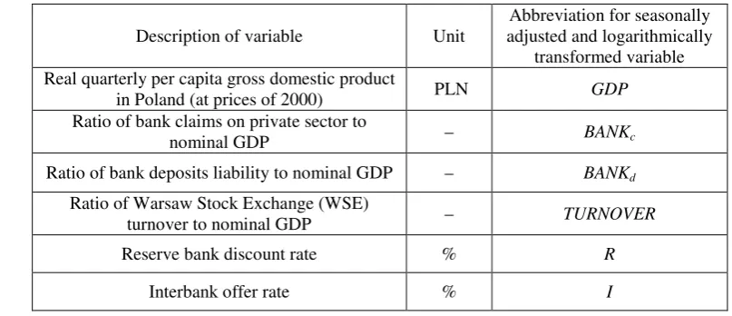
[image:6.595.88.492.559.733.2]variables. Table 1 contains some initial information.2
Table 1.
Units, abbreviations and a short description of examined variables
Description of variable Unit
Abbreviation for seasonally adjusted and logarithmically
transformed variable Real quarterly per capita gross domestic product
in Poland (at prices of 2000) PLN GDP Ratio of bank claims on private sector to
nominal GDP – BANKc
Ratio of bank deposits liability to nominal GDP – BANKd
Ratio of Warsaw Stock Exchange (WSE)
turnover to nominal GDP – TURNOVER
Reserve bank discount rate % R
Interbank offer rate % I
2
Details on applied dataset are presented in section 4.
At the very beginning of our computations we will check the stationarity of the time series listed in
Table 1. Stationarity is the main assumption of most statistical causality tests. Preliminary information
from the mass media and visual inspection of the dataset encouraged us to formulate the following:
Hypothesis 1: All time series under study are nonstationary.
The lack of stationarity suggests using the concept of cointegration or simply differencing the
respective time series. The applied tests allow us to establish the order of nonstationarity, i.e. to
determine the order of integration of the individual time series.
From economic literature it may be seen that the most common questions concerning
interdependencies between financial development and economic growth are the following:
•Does the banking sector cause economic growth or does causality run in the opposite direction?
•Do stock–market–related variables cause economic growth or does economic growth cause
stock market development?
•Is there a bilateral causal relationship (feedback) between banking sector development and
economic growth?
•Is there a bilateral causal relationship (feedback) between stock–market–related variables and
economic growth?
These questions concern both short and long run linear links as well as nonlinear relationships.
According to the Schumpeterian tradition banks stimulate economic growth. There are a number
of empirical contributions whose results support this point of view. However, in the more recent
literature the opposite direction of causality is also reported, i.e. the impact of economic growth on the
development of the banking system. This kind of economic thought is based on Robinson’s point of
view. It the light of the empirical results in the contributions reviewed, it seems that this point of view
may be true for highly developed countries. For countries like China and Greece feedback between
economic growth and the development of the banking system was reported. Causality running from
banking development to economic growth means that a better developed banking system finances
productive projects in a more successful way. An important result that clarifies the theoretical findings
is that causality is more marked in countries with a more developed institutional environment
(expressed by the rule of law and regulation). Feedback means that causality also runs from economic
growth to banking, which indicates that a more developed economy has a more developed banking
system. This implies, in particular, that credit for the private sector increases and the interest spread
diminishes as the economy develops. Both the Polish banking system and economic growth
experienced considerable expansion in the last decade. Therefore it is not easy to say in advance that
“finance leads growth” or that “finance follows growth”. Thus we formulate the following hypothesis:
Hypothesis 2: There was a feedback between the development of the banking system and
economic growth in Poland.
Most theoretical and empirical contributions report a significant causal relationship running from
stock market behaviour to economic growth. This observation is likely to be true also in the case of
the Warsaw Stock Exchange (WSE). Since July 2007 the WSE has experienced drops, although the
main macroeconomic indicators did not decline. Market participants were assured that drops in share
prices on the Warsaw stock market were of a temporary nature and did not detract from the good state
of the Polish economy. However, in the following year the condition of many Polish companies
worsened dramatically.
Large institutional investors (like banks or investment funds), which operate on the stock market
have good information about the financial state of companies and consumer demand. Insiders also
play an important role. Confidential information about an upcoming unprofitable event with respect to
a company or whole sector or just fear of crisis encourages the sale of equities. In consequence the
prices of shares decline and therefore a bear phase of the stock market begins. The companies have no
incentives to issue shares. Disposable capital is reduced, investment and, in consequence employment
decrease. Therefore output (GDP) and demand (consumption) also fall.
A different scenario takes place if the economic situation improves. Share issues start because
capital is demanded. This makes the development of companies, a rise in employment and a rise in
GDP possible.
According to the empirical contributions in the literature the more developed the country the
stronger the dependence between the stock market and the economic growth. Current movements on
the stock exchange determine the future economic situation.
In order to check the interdependence between turnover changes on the WSE and economic
growth we formulated the following:
Hypothesis 3: Turnover on the WSE Granger caused economic growth in Poland both in short
and long run.
As already mentioned Hypotheses 1-3 correspond to the pre-crisis (Q1 2000 - Q3 2008) period. The
last hypothesis refers to the impact of financial crisis of 2008 on the structure of financial sector-GDP
links in Poland. Since Poland was one of the few countries which managed to avoid serious economic
troubles after the bankruptcy of Lehman Brothers, one could formulate the following:
Hypothesis 4:Hypotheses 1-3 held true also for the full sample. In other words the structure of
causal links between financial sector and GDP in Poland was robust to the impact of financial
crisis of 2008.
The hypotheses listed above will be checked by some recent causality tests. The details of the testing
procedures will be shown in the following sections. The test outcomes depend to some extent on the
testing methods applied. Therefore, testing for the robustness of the empirical results is one of our
main tasks. Before describing the methodology, in the next section we will give description of the
time series included in our sample.
4. The Dataset and Its Properties
The major problem in most empirical studies is the selection of indicators reflecting the level of
financial development. The diversity of services involved makes the construction of financial
development indicators extremely difficult. Agents and institutions involved in financial
intermediation activities are also highly diversified, which causes additional difficulties. Taking into
consideration previous empirical studies (see e.g. Thangavelu and Ang, 2004; Shan and Morris, 2002)
we performed an investigation of the causal dependencies between economic growth and financial
development in Poland in the last decade using three indicators, namely the ratio of bank claims in the
private sector to nominal GDP, the ratio of bank deposit liability to nominal GDP, and the ratio of
Warsaw Stock Exchange turnover to nominal GDP. Therefore, our paper combines bank– and
market–based approaches for modelling the dynamic dependencies between GDP and the financial
sector.
Since the development of the financial sector and economic growth can be driven by a common
variable (Rajan and Zingales, 1998; Luintel and Khan, 1999; Dritsakis and Adamopoulos, 2004;
Thangavelu and Ang, 2004), we applied the interest rate as this common factor. Moreover, to examine
the stability of the links we used two types of interest rate – the reserve bank discount rate and the
interbank offer rate.
Further parts of this section contain statistical details on the data. Subsection 4.1 provides some
initial description of the variables under study. In subsection 4.2 the stationarity properties of all the
time series are examined. The identification of the orders of integration of the time series under study
is a crucial stage of causality analysis. If the precondition of stationarity is not fulfilled a standard
linear Granger causality test is likely to produce spurious results.3
4.1. Description of the Dataset
The dataset applied in this paper includes quarterly data on real per capita GDP (at constant prices of
year 2000), the ratio of bank claims in private sector to nominal GDP, the ratio of domestic bank
deposit liabilities to nominal GDP and the ratio of WSE turnover to nominal GDP in the period Q1
2000 – Q4 2011.4 Besides the GDP (measure of economic growth) and three measures of financial
development for bank–based (BANKc, BANKd) and market–based system (TURNOVER) two interest
rates (R, I) were applied to avoid the problem of the omission of important variables and additionally
to test the robustness of the empirical findings. Data on real GDP per capita, BANKc and BANKd was
3
Previous empirical (Granger and Newbold, 1974) and theoretical (Phillips, 1986) deliberations investigated this phenomenon in detail.
4
The dataset is provided by the authors in a separate file, which is downloadable from the Journal’s webpage.
obtained from Central Statistical Office in Poland, data on TURNOVER was gained from WSE
Monthly Bulletins. Finally data on R and I was gained from the National Bank of Poland.5
Since visual inspection of the unadjusted data provides a basis to claim that all variables (except
for the two interest rates) are most likely characterized by significant seasonality, and this feature
often leads to spurious results in causality analysis, the X-12 ARIMA procedure (which is currently
used by U.S. Census Bureau for seasonal adjustment) of Gretl software was applied to adjust the
variables. Finally, each seasonally adjusted variable was transformed into logarithmic form, since this
Box–Cox transformation may stabilize variance and therefore improve the statistical properties of the
data, which is especially important for parametric tests.
The application of quarterly data is important for two main reasons. First, since the data necessary
covered only the recent few years, a causality analysis based on annual data could not be carried out
due to lack of degrees of freedom.Moreover, as shown in some papers (Granger et al., 2000) the
application of lower frequency data (e.g. annual) may seriously distort the results of Granger causality
analysis because some important interactions may stay hidden.
A comprehensive preliminary analysis requires analysis of the charts for all the variables under
study. This may also provide some initial notion on the impact of financial crisis of 2008 on the
examined dataset. Figure 1 contains suitable plots of seasonally adjusted and logarithmically
transformed variables (as already mentioned seasonal adjustment was not required for R and I).
In the last decade there was relatively stable growth of the Polish economy, which is reflected in
the graph of GDP (upward tendency). One cannot forget that the Polish economy was one of the few
that managed to avoid an undesirable impact of the crisis of 2008. However, before 2002 (crisis of
2001) and after September 2008 one can observe a slight slowdown in the rate of growth of the Polish
economy.
5
Strictly speaking, R in quarter t is the rediscount rate measured at the end of period and I is the average of daily values of 3–Month Warsaw Interbank Offer Rate (WIBOR 3M) for a quarter t.
Figure 1. Plots of examined time series
Similarly, Figure 1 provides strong evidence for claiming that in the recent decade there was also
stable development of the financial sector in Poland. This is shown for the bank– (BANKc, BANKd)
and market–related (TURNOVER) variables. In contrast with economic growth, the financial sector in
Poland significantly reacted to the economic crises of 2001 and 2008. Figure 1 provides details about
significant drops in TURNOVER before 2002 and especially after September of 2008. The negative
impact of both economic crises is also demonstrated in plots of the ratios of bank claims in the private
sector and bank deposit liabilities to nominal GDP.
The plots of the last two examined time series describe some key aspects of the monetary policy
of the National Bank of Poland in the last decade. Both rates dropped from a level of about 20% in
year 2000 to a level of around 5% in year 2004. In general, starting from year 2004 both rates were
oscillating around 4.5%, reaching values of 4.75% (R) and 4.86% (I) in the last quarter of 2011. It
seems very likely that such large fluctuations in both types of interest rate should have an effect
(individual and mutual) on economic growth and on the performance of the financial sector in Poland
in years 2000–2011. Thus, we included these variables as additional (common) factors.
In the next subsection the preliminary analysis of the time series included in our dataset will be
extended by stationarity testing.
4.2. Stationarity Properties of the Dataset
Augmented Dickey–Fuller, Kwiatkowski–Phillips–Schmidt–Shin and Phillips–Perron tests were
applied to analyze stationarity properties of the time series under study. For each test we examined
two types of deterministic term (first one restricted to a constant and the other one containing constant
and linear trend). For the pre-crisis period all examined time series were found to be nonstationary at
a 5% significance level, regardless of the type of deterministic term, which clearly supported
Hypothesis 1.6 Some further calculations (conducted for first differences) confirmed that all the
variables under study are integrated of order one.7 Finally it should be noted, that all the variables
under study were found to be I(1) also for the full sample (covering period Q1 2000 – Q4 2011).
5. Methodology
In this paper several econometric tools were applied to test for both linear and nonlinear Granger
causality between GDP and financial development in the Polish economy. The main part of our
research was conducted in three variants, each of which involved GDP and one variable related to
financial sector (BANKc, BANKd and TURNOVER). As already mentioned, for the sake of the
correctness of computations (allowing control variables) and the robustness of the empirical results
two types of interest rate were also applied. Therefore, our analysis was based on six modelling
schemes. Each model was evaluated on the basis of pre-crisis data and the full sample.
6
For TURNOVER time series trend–stationarity was confirmed by the KPSS test, although the ADF and PP tests clearly rejected this posibility.
7
It should be underlined that detailed results of all computations which are not presented directly in the text in detailed form (usually to save space) are available from the authors upon request.
5.1. Linear Short and Long Run Granger Causality Tests
In this paper we applied three econometric methods suitable for testing for linear short and long run
Granger causality for nonstationary variables integrated in the same order, namely, the analysis of
unrestricted vector error correction model (VECM), the sequential elimination of insignificant
variables in VECM, and the Toda–Yamamoto procedure. Moreover, besides the asymptotic variant,
each procedure was additionally performed in a bootstrap framework. The application of such a
variety of methods is believed to ensure a verification of robustness and the validation of empirical
findings.
Since for both periods all variables under study were found to be I(1), the idea of cointegration
and analysis of unrestricted VEC model allowed an examination of both short and long run causal
dependencies. The finding that the variables are cointegrated implies the existence of long run
Granger causality in at least one direction (Granger, 1988). The simplest way to establish the direction
of causality is based on checking (using a t–test) the statistical significance of the error correction
terms in VECM. The test of joint significance (F–test) of lagged differences allows for short run
causality investigations.
The application of an unrestricted VEC model has one serious drawback, however. In order to
avoid the consequences of the autocorrelation of residuals it is often necessary to use a relatively large
number of lags, which may simultaneously reduce the number of degrees of freedom. This in turn
may have an undesirable impact on test performance, especially for small samples. Another problem
related to testing for linear causality using a traditional Granger test is multicollinearity, which is
especially significant for dimensions higher than two. For these reasons, a sequential elimination of
insignificant variables was additionally applied for each VECM equation separately. This procedure
sequentially omits the variable with the highest p–value (t–test) until all remaining variables have a p–
value no greater than a fixed value (in this paper it was 0.10).8
An alternative method for testing for linear Granger causality was formulated by Toda and
Yamamoto (1995). The prevalence of this method is due to the fact that it is relatively simple to
8
More technical details of this approach can be found in Gurgul and Lach (2010).
perform and free of complicated pretesting procedures, which may bias the test results, especially
when dealing with nonstationary variables (Gurgul and Lach, 2011). However, the key advantage is
the fact that this procedure is applicable even if the variables under study are characterized by
different orders of integration.9 On the other hand, the Toda–Yamamoto (TY) approach does not
allow us to distinguish between short and long run causal effects.10
All the aforementioned parametric methods have a few serious drawbacks. First of all, the
application of asymptotic theory requires specific modelling assumptions to hold true. Otherwise
spurious results may occur. Second, for extremely small samples the distribution of the test statistic
may be significantly different from an asymptotic pattern even if all modelling assumptions hold true.
One possible way of overcoming these difficulties is the application of the bootstrap method. By and
large, this procedure is used for estimating the distribution of a test statistic by resampling data. Since
the estimated distribution depends only on the available dataset, bootstrapping does not require such
strong assumptions as parametric methods. However, in some specific cases this concept is also likely
to fail, so it should not be treated as a perfect tool for solving all possible model specification
problems (Horowitz, 1995).
The bootstrap test applied in this paper was based on resampling leveraged residuals, because
such an approach may minimize the undesirable influence of heteroscedasticity. In recent years the
problem of the establishment of the number of bootstrap replications has attracted considerable
attention (Horowitz, 1995). The procedure of establishing the number of bootstrap replications
recently developed by Andrews and Buchinsky (2000) was applied in this paper. In all cases our goal
was to choose such a value of number of replications which would ensure that the relative error of
establishing the 10%–critical value would not exceed 0.05 with a probability equal to 0.95.11 All
aforementioned procedures were implemented using the Gretl software.
9
In such cases a standard linear causality analysis cannot be performed by the direct application of a basic VAR or VEC model. On the other hand, differencing or calculating the growth rates of some variables allows the use of the traditional approach, but it can also cause a loss of some information and lead to problems with the interpretation of results.
10
The long run dependencies between GDP and financial sector are especially important, as short run causal links may be related to business cycle or multiplier effects and die out without having lasting efects.
11
A detailed description of the resampling procedure applied in this paper may be found in Hacker and Hatemi (2006).
5.2. Nonlinear Granger Causality Test
The motivation to use nonlinear methods in testing for Granger causality is twofold. First, the
traditional linear Granger causality test was found to have very low power in detecting certain kinds
of nonlinear causal interrelations.12 Second, since linear tests are mainly based on checking the
statistical significance of suitable parameters only in a mean equation, testing for causality in any
higher–order structure (e.g. variance) is impossible (Diks and DeGoede, 2001).
The nonlinear causality testing procedure proposed by Diks and Panchenko (2006) was used in
this paper. We set up a common lag parameter (denoted as lDP) at a level of 1 and 2 while the
bandwidth (denoted as bDP) was set at the order of 0.5, 1 and 1.5.
13
A nonlinear causality is significant
if it was found for at least one combination of bDP and lDP. The detailed description of the role of these
technical parameters and the form of test statistic may be found in Diks and Panchenko (2006).
6. Empirical Results
This section contains the results of the short and long run linear Granger causality analysis as well as
the outcomes of nonlinear causality tests. The main goal of our empirical study was to examine the
research hypotheses presented in section 3. Outcomes presented in subsections 6.1-6.3 corespond to
the pre-crisis period while subsection 6.4 also discusses results obtained for the full sample. As
already mentioned, for both periods examined the reserach was performed on the basis of six
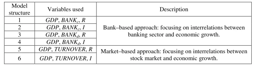
[image:16.595.89.505.544.651.2]schemes. Table 2 contains some initial details.
Table 2.
Specification of models applied in empirical study
Model
structure Variables used Description 1 GDP, BANKc, R
Bank–based approach: focusing on interrelations between banking sector and economic growth.
2 GDP, BANKc, I 3 GDP, BANKd, R 4 GDP, BANKd, I
5 GDP, TURNOVER, R Market–based approach: focusing on interrelations between stock market and economic growth.
6 GDP, TURNOVER, I
The empirical results presented in the following subsections are related in most cases only to an
examination of the causal links between economic growth and financial development. The results of
12
See, for example, Brock (1991). 13
These values have been commonly used in previous papers (see e.g. Diks and Panchenko (2006), Gurgul and Lach (2010)). Moreover, we applied discussed nonlinear procedure using all practical suggestions presented in Gurgul and Lach (2010).
testing for causality between interest rates and economic growth, as well as interest rates and financial
development are not the main focus of this study and hence they are not presented explicitly in the
text. However, some short remarks about the analysis of these links (less important for the subject of
the paper) in both periods under study are also made.
6.1. Results Obtained for Bank–Related Models Based on Pre-Crisis Data
The examination of causal dependencies between economic growth and financial development was
first performed for bank–related models. Since all variables examined in this part of the research
(GDP, BANKc, BANKd, R, I) were found to be I(1), a cointegration analysis was first performed.
6.1.1. Bank Claims and Economic Growth
Before conducting cointegration tests the type of deterministic trend was first specified using the five
possibilities listed in Johansen (1995). The results presented in subsection 4.2 (no trend–stationarity)
provided a basis to assume Johansen’s third case, that is the presence of a constant in both the
cointegrating equation and the test VAR. Next, we set the maximal lag length (for levels) at a level of
6 and then we established the appropriate number of lags using the information criteria (AIC, BIC,
HQ).
The results of both variants of Johansen’s test provided solid evidence to claim that GDP, each
bank–related variable and the interest rate are indeed cointegrated. All tests supported the hypothesis
that the dimension of cointegration space is equal to one at a 5% significance level.14 After performing
an analysis of the cointegration properties, we estimated suitable VEC models assuming 2 lags (for
levels) and one cointegrating vector in each case. Table 3 contains the p–values obtained while testing
for linear short and long run Granger causality using an unrestricted VEC model and the sequential
elimination of insignificant variables. Testing for causality in each direction was based on
asymptotic– and bootstrap–based critical values (bootstrap p–values are presented in square
brackets).15
14
In all testing variants the hypothesis that the smallest eigenvalue is equall to 0 was clearly accepted, which additionally validated the results of the previously performed unit root tests (Lütkepohl, 1993).
15
Throughout this paper the notation “x y” is equivalent to “x does not Granger cause y”. Moreover, the symbol “NCL” is the abbreviation of “no coefficients left”. Finally, bold face always indicates finding a causal link in a particular direction at a 10% significance level.
¬ →
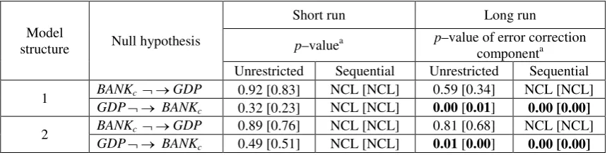
Table 3.
Analysis of causal links for model structure 1 and 2 (VEC–based approach) based
on pre-crisis data
Model
structure Null hypothesis
Short run Long run
p–valuea p–value of error correction componenta
Unrestricted Sequential Unrestricted Sequential
1 BANKc GDP 0.92 [0.83] NCL [NCL] 0.59 [0.34] NCL [NCL] GDP BANKc 0.32 [0.23] NCL [NCL] 0.00 [0.01] 0.00 [0.00]
2 BANKc GDP 0.89 [0.76] NCL [NCL] 0.81 [0.68] NCL [NCL] GDP BANKc 0.49 [0.51] NCL [NCL] 0.01 [0.00] 0.00 [0.00]
a
Number of bootstrap replications established by the Andrews and Buchinsky (2000) method varied between 2889 and 3739.
An analysis of the results presented in Table 3 leads to the conclusion that in the short run no causality
was detected. This result was found to be robust when exposed to VEC–based analysis as well as a
type of interest rate used. Similarly, the long run impact of GDP on BANKc was also found to be
robust to changes of testing procedure and the choice of control variable. On the other hand, evidence
of long run causality from BANKcto GDP was not suported neither by the results of an analysis of the
unrestricted VEC models nor any sequential variant.
For the sake of comprehensiveness the Toda–Yamamoto approach for testing for causal effects
between bank claims and economic growthwas additionally applied. The outcomes of this procedure
are presented in Table 4.
Table 4.
Analysis of causal links for model structure 1 and 2 (TY approach) based on
pre-crisis data
Model structure Parameters for TY procedurebNull hypothesis p–value
Asymptotic Bootstrapa
1 p1=2, p2=1 BANKc GDP 0.57 0.65 (N=3139) GDP BANKc 0.36 0.42 (N=3099)
2 p1=2, p2=1
BANKc GDP 0.44 0.51 (N=3479) GDP BANKc 0.62 0.54 (N=2759) a
Parameter N denotes the number of bootstrap replications established according to the Andrews and Buchinsky (2000)
procedure
.
b
Parameter p1 denotes order of the VAR model while parameter p2 stand for the highest order of integration of all examined
variables (Toda and Yamamoto, 1995).
In general, the results presented in Table 4 are in line with the outcomes contained in Table 3.
Causality was not reported in any direction, regardless of the type of critical values used.
In the last step of the causality analysis we performed nonlinear tests for three sets of residuals
resulting from linear models, that is the residuals of unrestricted VECM, the residuals resulting from
individually (sequentially) restricted equations and the residuals resulting from the augmented VAR
model applied in the Toda–Yamamoto method.16 For each combination of bDP and lDP three p–values
are presented: in the upper row the p–value for residuals of unrestricted VEC model (left) and p–value
for residuals of sequentially restricted equations (right) are presented. In the lower row the p–value
obtained after analysis of residuals of TY procedure is placed. Table 5 presents p–values obtained
while testing for nonlinear Granger causality between BANKc and economic growth. In all examined
[image:19.595.75.523.293.418.2]cases no filtering was used since no significant evidence of heteroscedasticity was found.17
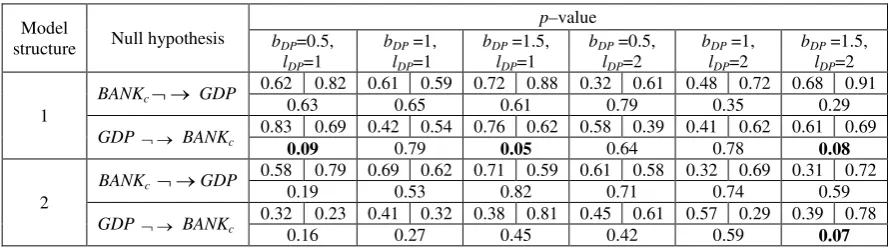
Table 5.
Analysis of nonlinear causal links for
BANK
cand
GDP
based on pre-crisis data
Model
structure Null hypothesis
p–value
bDP=0.5,
lDP=1
bDP =1,
lDP=1
bDP =1.5,
lDP=1
bDP =0.5,
lDP=2
bDP =1,
lDP=2
bDP =1.5,
lDP=2
1
BANKc GDP
0.62 0.82 0.61 0.59 0.72 0.88 0.32 0.61 0.48 0.72 0.68 0.91 0.63 0.65 0.61 0.79 0.35 0.29
GDP BANKc
0.83 0.69 0.42 0.54 0.76 0.62 0.58 0.39 0.41 0.62 0.61 0.69
0.09 0.79 0.05 0.64 0.78 0.08
2
BANKc GDP
0.58 0.79 0.69 0.62 0.71 0.59 0.61 0.58 0.32 0.69 0.31 0.72 0.19 0.53 0.82 0.71 0.74 0.59
GDP BANKc
0.32 0.23 0.41 0.32 0.38 0.81 0.45 0.61 0.57 0.29 0.39 0.78 0.16 0.27 0.45 0.42 0.59 0.07
As one can see, nonlinear causality running from GDP to the ratio of bank claims in the private sector
to nominal GDP was found for residuals resulting from post–TY residuals of both model structures.
On the other hand, nonlinear causality in the opposite direction was not reported in any research
variant.
To summarize, we found strong support to claiming that GDP causes BANKc both in the long and
short run. On the other hand, we found no evidence of causality running in the opposite direction. It is
important to note that in general both these findings were supported by the results of different
econometric methods (linear VEC–based and TY–based procedures supplemented with Diks and
Panchenko’s nonlinear test) and different choices of control variable. The stability of these results is
especially important in terms of the robustness and validation of empirical findings.
16
The residuals are believed to reflect strict nonlinear dependencies as the structure of linear connections had been filtered out after an analysis of linear models (Baek and Brock, 1992).
17
As stated in Diks and Panchenko (2006) the filtration of (conditional) heteroscedasticity may simply affect the dependence structure and consequently reduce the power of the test. Moreover, without knowing the true functional form of the process, a simple heteroscedasticity filter (like ARCH or GARCH model etc.) may not entirely remove the conditional heteroscedasticity in the residuals
6.1.2. Bank Deposit Liability and Economic Growth
This subsection contains results obtained after an analysis of causal dependencies between real per
capita GDP and the ratio of bank deposit liability to nominal GDP. At a 5% significance level both
variants of Johansen’s test provided solid evidence for claiming that for model structures 3 and 4 the
dimension of cointegration space is equal to two. As in the previous case (subsection 6.1.1) the
nonstationarity of all variables was confirmed once again. Next, we estimated a suitable VEC model
assuming 1 lag (for levels) and two cointegrating vectors to test for causality. As in previous
subsection, a TY procedure was additionally applied. Finally, a nonlinear test was applied to the
residuals resulting from all linear models. Table 6 contains a summary of results. Causality (non–
causality) at a10% significance level is marked in Table 6 by (). Symbols in square brackets refer
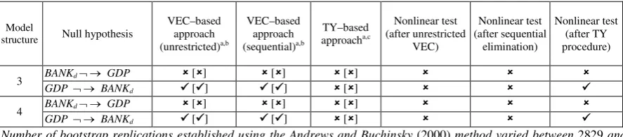
[image:20.595.77.521.389.487.2]to the results of bootstrap–based procedures.
Table 6.
Results of causality analysis for model structure 3 and 4 based on pre-crisis data
Model
structure Null hypothesis
VEC–based approach (unrestricted)a,b VEC–based approach (sequential)a,b TY–based approacha,c Nonlinear test (after unrestricted VEC) Nonlinear test (after sequential elimination) Nonlinear test (after TY procedure)
3 BANKd GDP [] [] []
GDP BANKd [] [] []
4 BANKd GDP [] [] []
GDP BANKd [] [] []
a
Number of bootstrap replications established using the Andrews and Buchinsky (2000) method varied between 2829 and
3839.
b
One lag (in levels) was found as optimal, thus short run causality could not be examined within a VECM framework.
c
Parameters for TY procedure: p1=1, p2=1.
In general, the results contained in Table 6 are in line with the results presented in previous
subsection. Swapping BANKc with BANKd did not change the conclusion that real per capita GDP in
Poland caused bank sector development in the short and long run in the last decade. On the other
hand, we found no evidence supporting causality running in the opposite direction. This way only
weak evidence supporting Hypothesis 2 was found. As in the previous subsection, all these empirical
findings were supported by the results of different econometric methods and different choices of
control variable, which surely validates our empirical findings.
¬ → ¬ →
¬ → ¬ →
6.2. Results Obtained for Stock Market–Related Models Based on Pre-Crisis Data
This subsection contains the results of the examination of causal dependencies between real per capita
GDP in Poland and the ratio of WSE turnover to nominal GDP. In other words, the dynamic links
between financial development and the economic growth of Poland in period Q1 2000 – Q3 2008
were examined within a stock market–based framework.
As in subsection 6.1, in the beginning a cointegration analysis was performed. First, we followed
the previously described preliminary procedure (selection of lag and the type of deterministic term).
The testing procedure was based on 2 lags (in levels) and the assumption of Johansen’s third case. At
a 5% significance level both variants of Johansen’s test provided solid evidence for claiming that for
model structures 5 and 6 the dimension of cointegration space is equal to one. After performing the
cointegration analysis, linear and nonlinear causality tests were also conducted. To ensure ease of
[image:21.595.77.522.421.513.2]interpretation and to save space the results are briefly presented in Table 7.
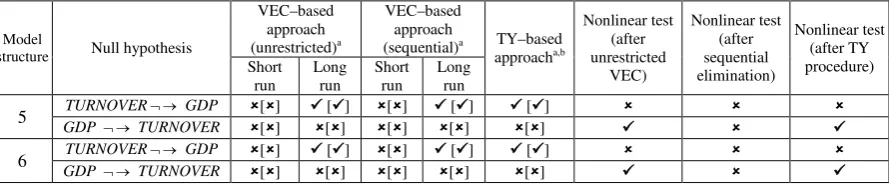
Table 7.
Results of causality analysis for model structure 5 and 6 based on pre-crisis data
Model
structure Null hypothesis
VEC–based approach (unrestricted)a
VEC–based approach
(sequential)a TY–based approacha,b Nonlinear test (after unrestricted VEC) Nonlinear test (after sequential elimination) Nonlinear test (after TY procedure) Short run Long run Short run Long run
5 TURNOVER GDP [] [] [] [] [] GDP TURNOVER [] [] [] [] []
6 TURNOVER GDP [] [] [] [] [] GDP TURNOVER [] [] [] [] []
a
Bootstrap–based results are presented in square brackets. Number of bootstrap replications established using the Andrews and Buchinsky (2000) method varied between 2669 and 3479.
b
Parameters for TY procedure: p1=2, p2=1.
As one can see, the results presented in this table lead to a different conclusion from the one drawn in
subsection 6.1. The real per capita GDP was found to be positively (comp. the plots of examined
variables) caused by TURNOVER both in the short and long run. This phenomenon was indicated
regardless of the choice of control variable and type of linear test applied, which provides clear
evidence of robustness. On the other hand, causality in the opposite direction was found to be much
less likely and possible only in the short run nonlinear sense. To summarize, Hypothesis 3 was clearly
6.3. Supplementary Results for Pre-Crisis Period
As already mentioned, the results of testing for causality between interest rates and economic growth,
as well as interest rates and financial development are not the main focus of this study and hence they
are not presented in details. Moreover, a number of the results obtained for the pairs GDPvs interest
rate and financial development vs interest rate were found to depend on the type of testing procedure
applied and the type of interest rate. However, there is a group of results which was found to be stable
and valid. We will briefly report these major observations.
For model structures 1–4 the interest rate was found to have a short and long run impact on
BANKcand BANKd. Evidence of causality running in the opposite direction was markedly weaker and
reported only in the nonlinear test. In general, a similar long run causal pattern was also found for real
per capita GDP and the interest rate within the framework of model structures 1–4. Moreover, solid
support for claiming that GDP caused both interest rates in the short run was also found, which
indicated the indirect short run impact from GDP to both bank–related variables. It is worth noting
that these indirect links were confirmed by testing direct causality between GDP and BANKc as well
as between GDP and BANKd (see subsection 6.1).
On the other hand, no causal links were found between the ratio of WSE turnover to nominal
GDP and either interest rate in both the short and long run. This lack of causality in any direction
implies that fluctuations in WSE turnover were not affected directly by the monetary policy of the
National Bank of Poland and vice versa. Moreover, it proves that in the period Q1 2000 – Q3 2008
dynamic relations between GDP, interest rates and financial development were not consistent for
different variables related to the financial sector in Poland.18
6.4. The Impact of 2008 Financial Crisis
In this subsection we focus on a comparison between outcomes obtained for pre-crisis-based models
(presented in subsections 6.1-6.3) and the full-sample-based ones. Using the all available data
18
These findings lead to the conclusion that development of stock market was an indirect causal factor for development of the banking sector in Poland in the last decade. Since this causal link is of great importance for a number of social groups in Poland (investors, bankers, policy makers, savers) we additionally performed an analysis of causal dependencies between both bank–related variables and TURNOVER within a two– dimensional framework. The results confirmed that TURNOVER causes BANKc and BANKd both in the short and long run. Evidence of causality in the opposite direction was markedly weaker (indicated only by nonlinear test).
(covering period Q1 2000 – Q4 2011) we repeated all the steps of empirical procedure including unit
root testing, cointegration analysis and short and long run linear and nonlinear causality tests.
As already mentioned, the results of unit root tests confirmed that all variables were I(1) also in
the period 2000-2011. In the next step we re-examined cointegration properties of all six models and
came to the conclusions that at 5% significance level the dimensions of cointegration spaces were
exactly the same for both periods. Finally, we rerun all causality tests for Q1 2000 – Q4 2011 period.
In order to save the space but also simultaneously highlight main differences between empirical
results obtained for both periods we present a brief comparison of outcomes of both research
[image:23.595.82.515.328.629.2]scenarios in Table 8:19
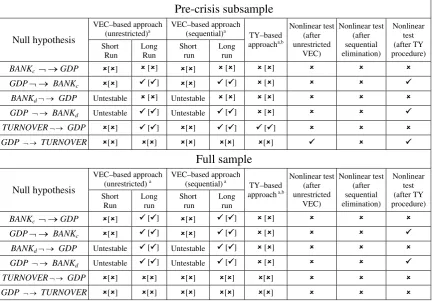
Table 8.
Comparison of results of causality analysis based on pre-crisis and full sample
Pre-crisis subsample
Null hypothesis VEC–based approach (unrestricted)a VEC–based approach (sequential)a TY–based approacha,b Nonlinear test (after unrestricted VEC) Nonlinear test (after sequential elimination) Nonlinear test (after TY procedure) Short Run Long Run Short run Long runBANKc GDP [] [] [] [] []
GDP BANKc [] [] [] [] []
BANKd GDP Untestable [] Untestable [] []
GDP BANKd Untestable [] Untestable [] []
TURNOVER GDP [] [] [] [] []
GDP TURNOVER [] [] [] [] []
Full sample
Null hypothesis
VEC–based approach (unrestricted) a
VEC–based approach (sequential) a
TY–based approach a,b
Nonlinear test (after unrestricted VEC) Nonlinear test (after sequential elimination) Nonlinear test (after TY procedure) Short Run Long run Short run Long run
BANKc GDP [] [] [] [] []
GDP BANKc [] [] [] [] []
BANKd GDP Untestable [] Untestable [] []
GDP BANKd Untestable [] Untestable [] []
TURNOVER GDP [] [] [] [] []
GDP TURNOVER [] [] [] [] []
a
Bootstrap–based results are presented in square brackets. Number of bootstrap replications established using the Andrews and Buchinsky (2000) method varied between 2949 and 3879.
b
Parameters for TY procedure: p1=2, p2=1 (except for the pair GDP and BANKd - in this case: p1=p2=1).
19
The summary of empirical results presented in Table 8 leads to several important conclusions. First of
all, we should mention that before the crisis of 2008 there was a unidirectional long run causality from
GDP to both bank-related variables while in the full period under study (also covering the crisis
period) the long run causality from BANKc and BANKd to GDP was also reported. On the other hand,
the long run causality from TURNOVER to GDP was not statistically significant for the full sample.
Both these findings provided evidence that Hypothesis 4 should clearly be rejected. To summarize,
the data presented in Table 8 provides a basis to claim that during the financial crisis of 2008 the
banking sector had much more significant impact on economic growth than before the crisis. On the
other hand, the causal impact of the performance of WSE on economic growth in Poland was
significant mostly for pre-crisis subsample. Finally it is worth to note that in general the outcomes of
an analysis of indirect links between financial-sector-related variables and GDP in period Q1 2000 –
Q4 2011 (through an analysis of causal links with R and I) were in line with results of testing the
direct causal links between BANKc, BANKd, TURNOVER and GDP.
7. Concluding Remarks
Most contributors have stressed that economic growth does not seem, as a rule, to depend on “prior”
changes in the financial system. Further deregulation of financial systems and financial institutions in
developed economies should improve and extend financial services. But this liberalization of policy
will not necessarily cause (in the Granger sense) a subsequent speeding up of economic growth.
Moreover, some economists think that financial crises might be caused by too intensive liberalization
of the financial sector, far in excess of the growth of the real sector. Other studies however are in line
with the conviction that financial development promotes economic growth, thus supporting the old
Schumpeterian hypothesis. The literature overview suggests that the link between financial
development and economic growth may be country–specific and probably depends on differences in
the industrial structures and cultures of societies.
In general, the results of the causality analysis performed for the pre-crisis subsample indicated
the existence of a significant unidirectional short and long run impact of real per capita GDP on both
bank–related proxies for financial development in Poland. These results were found to be robust to the
econometric method applied and the type of control variable used. Causality running from economic
growth to the banking sector may indicate that a more developed economy has a more developed
banking system. On the other hand, we found no evidence of causality running in the opposite
direction.
By contrast, causality tests performed for market–based models on the basis of the pre-crisis
subsample supported the existence of significant short and long run causality from financial
development to economic growth in Poland in the last decade. The robustness of this major finding
was also confirmed. In general, causality from real per capita GDP to the ratio of WSE turnover to
nominal GDP could not be confirmed by most of the tests applied, which led to serious doubts about
its existence.
To summarize, the empirical results provided evidence for claiming that before the crisis of 2008
the causal links between economic growth and the financial development of the Polish economy
strongly depended on the segment of financial sector. In general, we found that development of the
Warsaw Stock Exchange caused real per capita GDP growth and that economic growth caused the
development of the banking sector in Poland. These findings lead to the conclusion that the
development of the stock market was a causal factor for the development of the banking sector in
Poland in the last decade, which was also confirmed by direct causality tests performed within a two–
dimensional framework.
Research on the direction of causality between financial development and economic growth is
important because it has essential policy implications on the best economic strategy to enhance the
growth, in particular, of economies in transition. Financial development in Poland seems to stimulate
to some extent the economic growth of the country. Moreover, we can conclude (on the basis of the
dataset for Poland) that a better developed stock market leads to higher economic growth. This occurs
because the development of stock markets can imply risk diversification and better resource
allocation. Financial deregulation conducted in the period of transition improved competition and
allowed greater accessibility to financial products. Therefore we can take for granted that financial
deregulations in Poland in transition had a positive impact on economic growth.
In order to examine the impact of financial crisis of 2008 on financial sector-GDP causal links in
Poland we compared the results of the research performed for full sample (covering the period Q1
2000 – Q4 2011) and the pre-crisis subsample (Q1 2000 – Q3 2008). This comparison provided a
basis to claim that during the financial crisis of 2008 the banking sector had much more significant
impact on economic growth than before the crisis. On the other hand, the causal impact of the
performance of WSE on economic growth in Poland was significant mostly for the pre-crisis
subsample. The fact that positive causality running from TURNOVER to GDP was significant only
before the crisis means that during the crisis this causal impact could be significantly negative. This
important conclusion arises from the fact that the positive impact (reported for pre-crisis period) was
most likely cancelled out by negative shocks (observed in the crisis period), which in consequence led
to the lack of significant causalities in the full period.
We recognize, however, that our study might have inherent limitations. For example, our tests
could suffer from omitting some variables. Nevertheless, these probable drawbacks are likely to exist
in most, if not in all, time series analyses of this kind. The reason for this is lack of sufficient dataset.
In our opinion, future time series analyses should examine whether banking and stock markets are
related to certain components of GDP, such as investments, or to certain intensive sectors on the
supply side of the economy, such as the manufacturing industry.
Finally, we believe that our study provides a basis for further time series quantitative
investigations of the historical and contemporary role of banking and the stock market in the
economic development of Poland and other countries in transition.
References
[1]Abu–Bader S, Abu–Qarn AS (2008): Financial Development and Economic Growth: The Egyptian
Experience. Journal of Policy Modeling, 30: 887–898.
[2]Al–Awad M, Harb N (2005): Financial development and economic growth in the Middle East. Applied
Financial Economics, 15: 1041–1051.
[3]Andrews DWK, Buchinsky M (2000): A Three–Step Method for Choosing the Number of Bootstrap
Repetitions. Econometrica, 68, 23–52.
[4]Baek E, Brock W (1992): A general test for Granger causality: Bivariate model. Technical Report, Iowa
State University and University of Wisconsin, Madison.
[5]Bagehot W (1873): Lombard Street. Reprinted (1962): Homewood, IL: Irwin, R.D.
[6]Beck T, Levine R (2004): Stock Markets, Banks and Growth: Panel Evidence. Journal of Banking and
Finance, 28: 423–442.
[7]Brock W (1991): Causality, chaos, explanation and prediction in economics and finance. In: Casti J,
Karlqvist A (eds.): Beyond Belief: Randomness, Prediction and Explanation in Science. CRC Press, Boca
Raton, Fla., 230–279.
[8]Deidda L, Fattouh B (2002): Non–linearity between finance and growth. Economics Letters, 74: 339–345.
[9]Demetriades PO, Hussein AK (1996): Does financial development cause economic growth? Time series
evidence from 16 countries. Journal of Development Economics, 51: 387– 411.
[10]Diks CGH, DeGoede J (2001): A general nonparametric bootstrap test for Granger causality. In: Broer
HW, Krauskopf W, Vegter G (eds.): Global analysis of dynamical systems. Bristol, Institute of Physics
Publishing, 391–403.
[11]Diks CGH, Panchenko V (2006): A new statistic and practical guidelines for nonparametric Granger
causality testing. Journal of Economic Dynamics and Control, 30: 1647–1669.
[12]Dritsakis N, Adamopoulos A (2004): Financial Development and Economic Growth in Greece: An
Empirical Investigation with Granger Causality Analysis. International Economic Journal, 18: 547–559.
[13]Dritsaki C, Dritsaki–Bargiota M (2006): The Causal Relationship between Stock, Credit Market and
Economic Development: An Empirical Evidence for Greece. Economic Change and Restructuring, 38: 113–
127.
[14] Evans A, Green C, Murinde V (2002): Human capital and financial development in economic growth: new evidence using translog production function. International Journal of Finance and Economics, 7: 123–140.
[15]Fase MMG, Abma RCN (2003): Financial environment and economic growth in selected Asian countries.
Journal of Asian Economics, 14: 11–21.
[16]Granger CWJ, Newbold P (1974): Spurious regression in econometrics. Journal of Econometrics, 2: 111–
120.
[17]Granger CWJ (1988): Some recent developments in the concept of causality. Journal of Econometrics, 39:
199–211.
[18]Granger CWJ, Huang B, Yang C (2000): A bivariate causality between stock prices and exchange rates:
evidence from recent Asian Flu. The Quarterly Review of Economics and Finance, 40: 337–354.
[19]Gurgul H, Lach Ł (2010): The causal link between Polish stock market and key macroeconomic
aggregates. Betriebswirtschaftliche Forschung und Praxis, 4: 367–383.
[20]Gurgul H, Lach Ł (2011): The role of coal consumption in the economic growth of the Polish economy in transition. Energy Policy, 39: 2088-2099.
[21]Hacker RS, Hatemi–J A (2006): Tests for causality between integrated variables using asymptotic and
bootstrap distributions: theory and application. Applied Economics, 38: 1489–1500.
[22]Hicks J (1969): A theory of economic history. Clarendon Press, Oxford.
[23]Horowitz JL (1995): Bootstrap methods in econometrics: Theory and numerical performance. In: Kreps
DM, Wallis KF (eds.): Advances in Economics and Econometrics: Theory and Applications. Cambridge,
Cambridge University Press, 188–232.
[24]Johansen S (1995): Likelihood–based Inference in Cointegrated Vector Autoregressive Models. Oxford
University Press, Oxford.
[25]Kemal AR, Qayyum A, Hanif MN (2007): Financial Development and Economic Growth: Evidence from
a Heterogeneous Panel of High Income Countries. The Lahore Journal of Economics, 12: 1–34.
[26]Lopez–de–Silanes F, Glaeser E, La Porta V, Shleifer A (2004): Do Institutions Cause Growth? Journal of
Economic Growth, 9: 271–303.
[27]Lucas RE (1988): On the Mechanics of Economic Development. Journal of Monetary Economics, 22: 3–
42.
[28]Luintel KB, Khan M (1999): A quantitative reassessment of the finance–growth nexus: Evidence from a
multivariate VAR. Journal of Development Economics, 60: 381–405.
[29]Lütkepohl H (1993): Introduction to Multiple Time Series Analysis, second ed., Springer–Verlag, New
York.
[30]Phillips PCB (1986): Understanding the spurious regression in econometrics. Journal of Econometrics, 33:
311–340.
[31]Rajan RG, Zingales L (1998): Financial dependence and growth. American Economic Review, 88: 559–
586.
[32]Robinson J (1952): The Generalization of General Theory and other essays. Macmillan, London.
[33]Schumpeter JA (1934): Theorie der Wirtschaftlichen Entwicklung [The theory of economic development].
Leipzig: Dunker & Humblot, (1912); translated by Redvers Opie. Cambridge, MA: Harvard U. Press.
[34]Shan J, Morris A, Sun F (2001): Financial development and economic growth: an egg–and–chicken
problem. Review of international Economics, 9: 443–454.
[35]Shan J, Morris A (2002): Does financial development lead economic growth? International Review of
Applied Economics, 16: 153–168.
[36]Shan J (2005): Does financial development ‘lead’ economic growth? A vector autoregression appraisal.
Applied Economics, 37: 1353–1367.
[37]Shan J, Jianhong Q (2006): Does Financial Development ‘lead’ Economic Growth? The case of China.
Annals of Economics and Finance, 1: 231–250.
[38]Sinha D, Macri J (2001): Financial development and economic growth: the case of eight Asian countries.
Economia Internazionale, 54: 219–234.
[39]Tang D (2006): The effect of financial development on economic growth: evidence from the APEC
Countries, 1981–2000. Applied Economics, 38: 1889–1904.
[40]Thangavelu SM, Ang JB (2004): Financial Development and Economic Growth in Australia: An
Empirical Analysis. Empirical Economics, 29: 247–260.
[41]Toda HY, Yamamoto T (1995): Statistical inference in vector autoregressions with possibly integrated
processes. Journal of Econometrics, 66: 225–250.
[42]Zang H, Kim YC (2007): Does financial development precede growth? Robinson and Lucas might be
right. Applied Economics Letters, 14: 15–19.