A time scale analysis of systematic risk: wavelet based approach

Munich Personal RePEc Archive

A time-tcale analysis of systematic risk:

wavelet-based approach

Khalfaoui Rabeh, K and Boutahar Mohamed, B

GREQAM d’Aix-Marseille, IML université de la méditerranée

28 June 2011

Online at

https://mpra.ub.uni-muenchen.de/31938/

A Time-Scale Analysis of Systematic Risk: Wavelet-Based Approach

R. Khalfaoui∗and M. Boutahar†

Abstract

The paper studies the impact of different time-scales on the market risk of individual stock market returns and of a given portfolio in Paris Stock Market by applying the wavelet analysis. To investigate the scaling properties of stock market returns and the lead/lag relationship between them at different scales, wavelet variance and cross-correlations analyses are used. According to wavelet variance, stock returns exhibit long memory dynamics. The wavelet cross-correlation analysis shows that comovements between stock returns are stronger at higher scales (lower frequencies); scales corresponding to period of 4 months and longer, i.e. scales 7 and 8. The wavelet analysis of systematic risk shows that all individual assets and the diversified portfolio have a multi-scale behavior, which indicates that the systematic risk measured by Beta in the market model is not stable over time. The analysis of VaR at different time scales shows that risk is more concentrated at higher frequencies dynamics (lower time scales) of the data.

JEL Classification:C02; G12; G32

keywords:Wavelets, Systematic risk, Value-at-Risk

1

Introduction

There are several methods for analyzing financial time series, most of them used the time domain in econometric modeling. A natural concept in financial time series is the notion of multiscale features. That is, an observed time series may contain several structures, each occurring on a different time scale. Wavelet method was applied to separate the dynamics in a time series over a variety of different time horizons. Hence, wavelet analysis provides an efficient way to localize changes across time scales while maintaining the entropy conservation. This local property makes wavelets a suitable tool for analyzing economic and financial stochastic processes. Therefore, by decomposing a time series on different scales, one may expect to obtain a better understanding of the data generating process as well as dynamic market mechanisms behind the time series.

In recent years the interest for wavelet methods has increased in economics and finance. Ramsey and Zhang(1997) analyzed foreign exchange data using waveform dictionaries, Kim and In (2005) studied the relationship between stock markets and inflation using maximum overlap discrete wavelet transform estimator of the wavelet correlation.

In and Kim(2006) examined the relationship between Australian stock and futures markets over various time

hori-zons. Sharkasi et al.(2006) used wavelet transform to analyze the reaction of stock markets to crashes and events in emerging and mature markets, Kim and In (2007) studied the relationship between changes in stock prices and bond yields in the G7 countries.Durai and Bhaduri(2009) studied the relationship between stock prices, inflation and output using maximum overlap discrete wavelet transform.

In the area of finance, wavelet analysis appears useful, as different traders view the market with different time reso-lutions, for example hourly, daily, weekly or monthly. Markets consist of agents working in different time horizons. Therefore, the dynamics of interrelation between markets consist of scales that possibly behave differently. Different

∗_{GREQAM laboratory, University of Mediterranean II, 2 rue de la charité Marseille 13002. FRANCE. e-mail: [email protected]}

†_{IML, University of Mediteranean II, Faculty of science of Luminy, 163 Luminy Avenue Marseille 13288. FRANCE. e-mail:}

types of traders analyze the multi-scale dynamics of time series. In fact, they analyzed the risk management at differ-ent time-horizon and tried to find the corresponding investmdiffer-ent strategies.1 Norsworthy et al.(2000) analyzed stocks from the US market and find that beta coefficients generally decrease as we move into higher scales. Some studies applied wavelet-based risk analysis for estimating Value-at-Risk of time series. Gençay et al.(2005) proposed a new method to estimate systematic risk (the Beta) using multiscale decomposition through wavelet filters. Their findings in US, UK and Germany markets provides a stronger relationship between portfolio return and risk as the scale in-creases. Fernandez (2006) used wavelet analysis to test multiscale CAPM using portfolio from emerging markets and find that beta coefficient changes with different time scales.Heni and Boutahar(2011) focused on modelling the conditional mean and conditional variance of exchange rates. They estimated the GARMA-FIGARCH model using the wavelet-based maximum likelihood estimator.

Others studies are based on analyzing market risk by estimating Value at Risk at different time scales. Masih et al.

(2010) analyzed stocks from emerging Gulf Cooperation Council (GCC) equity markets and found that VaR measured at different time scales suggests that risk tends to be concentrated more at the higher frequencies of the data.

This paper is organized as follows: In section 2, wavelet analysis is explained. In section 3, we provide wavelet Value-at-Risk methodology. In section 4, we defined the Wavelet-Market Model. Empirical results are discussed in section 5. An extension is given in section 6. We conclude in section 7.

2

Wavelets

2.1 The Maximal Overlap Discrete Wavelet Transform

An alternative wavelet transform for the discrete wavelet transform (DWT)2of a time series is the Maximal Overlap Discrete Wavelet Transform (MODWT). Unlike the classical DWT, the MODWT is a non-orthogonal transform. It has many advantages over the DWT such as non-dyadic length sample size, invariant translation (i.e. shifting the time series by an integer unit will shift the MODWT wavelet and scaling coefficients the same amount), provides in-creased resolution at coarser scales and produces more asymptotically efficient wavelet variance estimator than DWT

(seePercival(1995)). The MODWT goes by several names in the statistical and engineering literature , such as, the

"stationary DWT" (Nason and Silverman(1995)), "translation-invariant DWT" (Coifman and Donoho(1995)), and "time-invariant DWT" (Pesquet et al.(1996)).

Percival and Walden (2000) define the MODWT of a time series Xt, t=1, . . . , N as follows: for an even

posi-tive inetegr L(Ldenotes the width of the initial filter), let{hl; l=0, . . . , L−1}and{gl; l=0, . . . , L−1}be the

Daubechies wavelet and scaling filters, respectively. The MODWT wavelet and scaling coefficients are the solutions of multiresolution decomposition analysis (pyramid algorithm3) ofMallat(1989). Thus, we have

˜

ωjt=

Lj−1

∑

l=0

˜

hjlXt−l mod N,t=0,1, . . . ,N−1, (2.1)

and

˜

νjt= Lj−1

∑

l=0

˜

gjlXt−l mod N, t=0,1, . . . ,N−1, (2.2)

whereLj≡(2j−1)(L−1) +1 is the length of the wavelet filter (seeGençay et al.(2002) for more detail) and where

the MODWT wavelet and scaling filters ˜hjl and ˜gjlare calculated by rescaling the DWT filters coefficients, such that

1_{Investors work on many different time scales, and with wavelets we can separate these different time scales. Investors should take into}

account also their investment horizon when they make risk management and portfolio allocation decisions. 2_{SeePercival and Walden(2000) for more details.}

F re q u e n c y Time Time F re q u e n c y

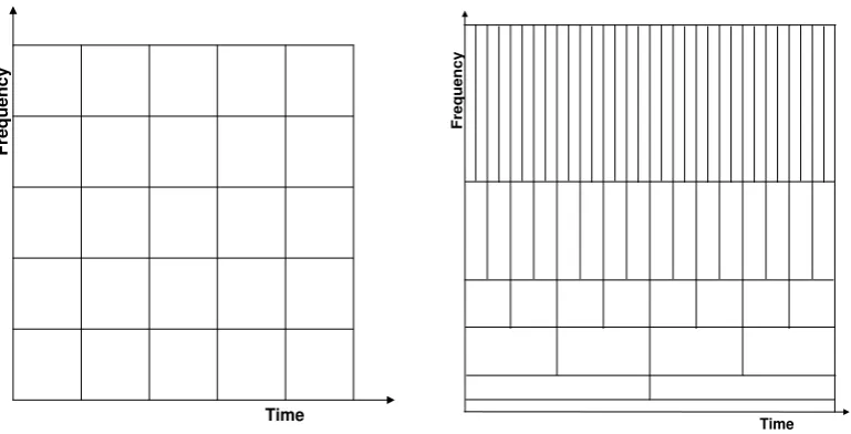
Figure 2.1 The short-time Fourier transform (left panel) and the wavelet transform (right panel) partitioning of the time–frequency plane.

˜

hjl=hjl/2j/2and ˜gjl=gjl/2j/2and circularly shifting by unit intervals for all levels of the transform. The MODWT

filters satisfies the following three properties:

L−1

∑

l=0

˜ hl=0,

L−1

∑

l=0

˜

gl=1, (2.3)

L−1

∑

l=0

˜ h2_jl=

L−1

∑

l=0

˜ g2_jl= 1

2j, (2.4)

∞

∑

l=−∞

˜

hlh˜l+2n= ∞

∑

l=−∞

˜

glg˜l+2n=0. (2.5)

Figure. 2.1 shows the time-frequency resolution properties of the Gabor transform or short-time (time-variable) Fourier transform and the wavelet transform. The gabor transform (left panel) has constant resolution at all times and frequencies and the wavelet transform provides good frequency resolution (and poor time resolution) at low frequencies and good time resolution (and poor frequency resolution) at high frequencies.4

2.2 Wavelet variance, covariance and correlation

2.2.1 Analysis of variance

Because wavelet transform can break down the original time series into components of different scales, it provides a powerful tool to detect the pattern of variations in observed data. In particular, it is interesting to calculate the wavelet variance on scale-by-scale basis.Percival(1995) andPercival and Mofjeld(1997) proved that the variance of a given time series is captured by the variance of the MODWT coefficients. Hence, the total variance of a time series can be partitioned using the MODWT as

kXk2= J

∑

j=1 ω˜_j

2

+kν˜Jk2. (2.6)

4_{Both Gabor and wavelet transform are based on Fourier transform. The Gabor transform uses constant window-function which cannot face}

where ω˜_j 2

is the detail variance (variance of X due to changes at scales λj) and kν˜Jk2 is the smooth variance

(variance due to changes at scalesλJ). The wavelet-variance analysis consists of partitioning the variance of a time

seriesXt into pieces that are associated to different time scales. It tells us what scales are important contributors to the

overall variability of a series (seePercival and Walden(2000) andGençay et al.(2002)). The wavelet variance of the wavelet coefficients ˜ωjtat scaleλjis defined as

˜

σ2 X(λj) =

1 2λj

Var(ω˜jt), (2.7)

where ˜ωjtis defined in equation (2.1) and scaleλj is associated with frequency interval

1/2j+1,1/2j. The total variance ofX can be decomposed as

J

∑

j=1

˜

σ_X2(λj) =Var(Xt). (2.8)

Mondal and Percival(1995) defined an unbiased MODWT estimator of ˜σ2

X(λj)as follows

ˆ

σ_X2(λj) =

1 Mj

N

∑

t=Lj

˜

ω2_jt, (2.9)

whereMj=N−Lj+1 is the number of maximum overlap coefficients andLj= (2j−1)(L−1) +1 is the length of

the wavelet filter.

Given the usefulness of the wavelet variance for univariate time series, the following section investigates thewavelet covarianceandwavelet correlationfor bivariate time series.

2.2.2 Analysis of covariance

To determine the relationship between two time series on a scale-by-scale basis the notion of wavelet covariance has to be used. Whitcher et al.(2000a) has been introduced the definition of wavelet covariance and wavelet correlation between two processes. LetXt andYt be two stationary discrete time series, and let ˜ωX,jt and ˜ωY,jt be the scale λj wavelet coefficients computed from applying MODWT to each time serisXt andYt, respectively. The wavelet

covariance of(Xt,Yt)for scaleλjis defined as

γXY(λj) =

1 2λj

Cov(ω˜X,jt,ω˜Y,jt). (2.10)

An unbiased estimator of the wavelet covariance based upon the MODWT is given by

ˆ

γXY(λj) =

1 Mj

N

∑

t=Lj

˜

ωX,jtω˜Y,jt (2.11)

By introducing an integerτ between ˜ωX,jt and ˜ωY,jt,Whitcher et al.(2000a) defined thewavelet cross-covarianceof (Xt,Yt)for a scaleλj and lagτas

γXY,τ(λj) =

1 2λj

Cov(ω˜X,jt,ω˜Y,j,t+τ). (2.12)

Return

Pr

o

b

a

b

il

ity

d

e

n

s

ity

VaR(1%)

1%

Profit/Loss

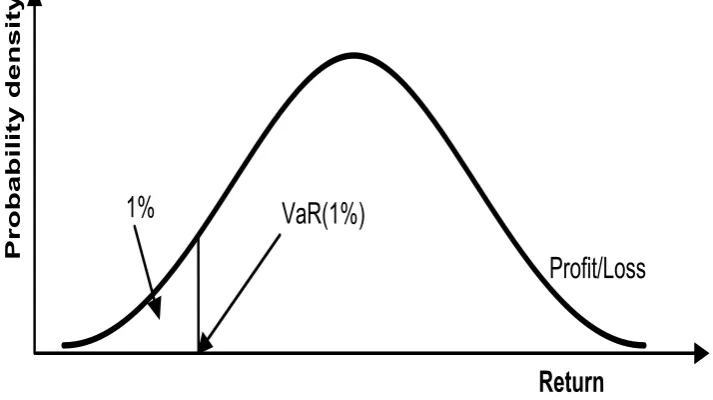
Figure 3.1 Value-at-Risk quantification using the normal probability density function

The MODWT wavelet cross-correlation coefficients for a scaleλjand lagτare simply obtained by using the wavelet

cross-covarianceγXY,τ(λj)and the standard deviations ˜σX2(λj)and ˜σY2(λj):

ρXY,τ(λj) =

γXY,τ(λj)

˜

σX(λj)σ˜Y(λj)

(2.13)

where ˜σ2

X(λj)and ˜σY2(λj)are the MODWT wavelet variance defined in equation (2.7). The wavelet cross-correlation

is used to determine lead/lag relationships on a scale by scale between two time series.

3

Value at Risk: VaR

Measure of risk management is the interest of traders in financial markets. There are many types of measures of risk, such that volatility, semi-variance or downside risk and expected shortfall. One of the most important risk measures in finance is the VaR, which measures the maximum trading loss that a bank can face over a given horizon (usually one day) and under a specified significance level (popular significance levels usually are 99% and 95%).5Considerpt, the

value of a given portfolio P at a particular timet(for example, dayt). Letrt be the return of this portfolio during the

period(t−1,t). The VaR is interpreted as the maximum loss of the portfolio not exceeded with a given probability over the period(t−1,t). Mathematically, VaR is defined at the period time∆tand for significance levelα% as

P(rt≤VaR(α)) =α, (3.1)

From the equation (3.1) and Figure 3.1 we observed that VaR estimates the statistically significant losses at the distribution tails.

Several methods for VaR estimation are discussed in the literature.6 These methods are grouped in three categories: non-parametric methods (Historical Simulation, Weighted Historical Simulation, Filtered Historical Simulation, ...), semi-parametric methods (extreme value theory, ...) and parametric methods (ARCH, univariate GARCH, multivariate GARCH, RiskMetrics). When looking at the time-varying volatility models for VaR estimation, one can see that these methods look at the historical data of the time-horizon chosen. Therefore, a tool is needed which enables the analyst

to decompose the signal into all of its components, separating higher frequent behavior from the lower frequent one, in order to analyze which of these components produce relevant information. The wavelet VaR fills this gap.

4

The Wavelet-market model

The market price is influenced by different market participants, such as intraday traders, daily traders, short term traders and long term traders. These participants have different trading strategies over different investment time-horizons. Therefore, market prices are formed by the influence of financial participants which caracterized by different time-frequencies. Thus, the market risk has a multi-scale structure. Most of the traders used a constant risk over a period (day, ...). In this section we introduced a market model at different scales: The Wavelet-market model. After decomposing a return series into jcrystals j=1, . . . ,J(details and smooths), The decomposition is based on MODWT using Mallat’s algorithm

rt=D1(t) +. . .+DJ−1(t) +DJ(t) +SJ(t). (4.1)

whereSJ(t)andDj(t),j=1, . . . ,Jare defined as follows

SJ(t) =

∑

sJkφJk(t), (4.2)

Dj(t) =

∑

djkψjk(t), j=1, . . . ,J. (4.3)

whereφjk(t)andψjk(t)are the father and mother wavelet that are given by the following two equations.7 jandkare

the number of scale crystals (intervals or frequencies) and the number of coefficients in each component.

φjk(t) =2−j/2φ

t−2jk 2j

f or j=1, . . . ,J (4.4)

ψjk(t) =2−j/2ψ

t−2jk 2j

f or j=1, . . . ,J (4.5)

To define the Wavelet-market model we run an Ordinary Least Square regression of each stock crystals on each crystals of the market portfoliorm:

rit(λj) =αi(λj) +βi(λj)rmt(λj) +εit(λj), j=1, . . . ,J. (4.6)

whererit(λj)andrmt(λj)are the details at scale(λj)of the assetiand the market return. In the Wavelet-market model

(equation 4.6 ), the wavelet beta estimator for asseti, at scaleλj, is defined as

ˆ

βi(λj) =

ˆ

γrirm(λj)

ˆ

σ2 rm(λj)

, j=1, . . . ,J. (4.7)

where ˆγrirm(λj)and ˆσ 2

rm(λj)are defined in (2.11) and (2.9). We define also, the waveletR

2 _{coefficient for asseti, at}

scaleλj, as

R2_i(λj) =βˆi2(λj)

ˆ

σ2 rm(λj)

ˆ

σ2 ri(λj)

, j=1, . . . ,J. (4.8)

From the Wavelet-market model, the market risk of a given asseti, at scale(λj), is decomposed to systematic risk and

unsystematic risk (independent of the market), thus we write

σ2

i(λj) =βi2(λj)σm2(λj) +σεi2(λj),i=1, . . . ,N j=1, . . . ,J. (4.9)

whereβ2

i (λj)σm2(λj)andσεi2(λj)are the systematic and unsystematic risks, at scaleλj, respectively.

For a given portfolioPofNassets, the wavelet variance-covariance matrix of theNasset returns, at scaleλjis defined

as follows

Σ_P(λj) =β(λj)β

′

(λj)σm2(λj) +Σε(λj), j=1, . . . ,J. (4.10)

whereβ(λj) = 

    

β1(λj) β2(λj)

.. .

βN(λj) 

    

andΣ_ε(λj) = 

    

σ2

ε1(λj) 0 · · · 0 0 σ2

ε2(λj) · · · 0 ..

. ... . .. ...

0 0 · · · σ2

εN(λj) 

    

, j=1, . . . ,J.

Assume thatE(rP) =0, the Wavelet-VaR of the portfolioPis given by

VaRλj(α) =F−1(α) q

κ′Σ_P(λj)κ, j=1, . . . ,J. (4.11)

whereκis aN×1 vector of portfolio weights andF−1(α)is the inverse of the cumulative normal distribution function. For an equally weighted portfolio, such thatκi=1/N∀i, the Wavelet-VaR is

VaR_λj(α) =F−1(α)





 σ2

m(λj) N

∑

i=1

βi(λj)/N !2

+ 1

N2 N

∑

i=1 σ2

εi(λj) 



 1/2

, j=1, . . . ,J. (4.12)

For a well-diversified portfolio, i.e. N is large, the Wavelet-VaR is approximately calculated by the systematic risk, such that we have

VaRλj(α)≈

1 NF

−1_(α)σ m(λj)

N

∑

i=1 βi(λj)

, j=1, . . . ,J. (4.13)

5

Data and empirical results

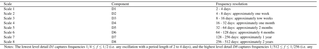
In this section, our analysis is based on stock market price of ten assets from Paris Stock Market. We decompose the returns series into their time-scale components using the MODWT analysis based on the Daubechies least asymmetric (LA) wavelet filter of lengthL=8.8 For any given time series, the level jwavelet coefficients are associated with changes at scaleλj=2j−1. Hence, the scale 2j−1corresponds to frequencies in the interval f ∈

1/2j+1,1/2j, the wavelet coefficient (detail) ˜ω1 associated with changes on the scale λ1 captures frequencies f ∈[0.25,0.5], thus is

associated to 2-4 days periods, similarly ˜ω2contains frequencies f∈[1/8,1/4], is associated with a period length of

4 to 8 days. While scalesλ3 toλ8 are associated to 8-16, 16-32, 32-64, 64-128, 128-256 and 256-512 day periods, respectively.

8_{It has been shown that LA(8) filter gives the best performence for the wavelet time series decomposition. This wavelet filter has been}

5.1 Data

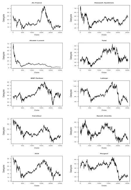
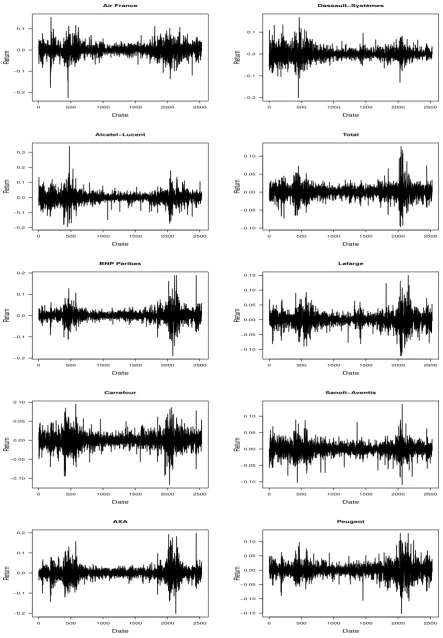
The data employed are daily closing stock market price for ten assets of many different sectors that are listed in France SBF 120 stock market Index, obtained from DataStream. The sample period runs from December 29, 2000 to September 06, 2010 (2529 observations). Table 5.1 shows additional information about the data used. For each stocki, we collect daily returns series, defined as returns of daily closing pricepit: rit =ln(pit)−ln(pi,t−1). Figure

5.1 depicts Level price series for the data and Figure 5.2 shows growth in the return series for all the stock prices.

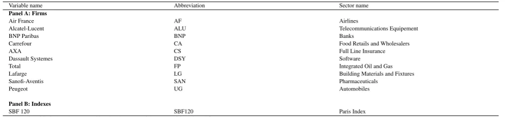
Table 5.1

Definition of variables used in the study

Variable name Abbreviation Sector name

Panel A: Firms

Air France AF Airlines

Alcatel-Lucent ALU Telecommunications Equipement BNP Paribas BNP Banks

Carrefour CA Food Retails and Wholesalers AXA CS Full Line Insurance Dassault Systemes DSY Software Total FP Integrated Oil and Gas Lafarge LG Building Materials and Fixtures Sanofi-Aventis SAN Pharmaceuticals

Peugeot UG Automobiles

Panel B: Indexes

SBF 120 SBF120 Paris Index Note: The table depicts the names, abbreviated names and the setors of the selected firms.

Table 5.2

Basic statistics for return series Panel A: Descriptive statistics

Air France

Alcatel-Lucent

BNP Paribas

Carrefour AXA Dassault Systèmes

Total Lafarge Sanofi-Aventis

Paugeot SBF120 Mean (%) -0.032 -0.130 0.007 -0.022 -0.040 -0.015 -0.0001 -0.024 -0.016 -0.024 -0.015 Std.dev. 0.027 0.035 0.024 0.018 0.029 0.025 0.017 0.022 0.018 0.022 0.015 Maximum 0.154 0.340 0.189 0.094 0.198 0.168 0.127 0.150 0.136 0.129 0.103 Minimum -0.225 -0.194 -0.189 -0.116 -0.202 -0.200 -0.096 -0.121 -0.109 -0.152 -0.093 Skewness -0.305 0.145 0.320 -0.150 0.357 0.113 0.137 -0.0005 -0.008 0.044 0.049 Kurtosis 5.096 7.430 9.637 3.976 6.731 5.488 5.940 4.866 4.354 4.010 5.617 JB testp−value 0.000∗ 0.000∗ 0.000∗ 0.000∗ 0.000∗ 0.000∗ 0.000∗ 0.000∗ 0.000∗ 0.000∗ 0.000∗ LBp−value 0.023∗ 0.000∗ 0.000∗ 0.000∗ 0.000∗ 0.000∗ 0.000∗ 0.000∗ 0.000∗ 0.000∗ 0.000∗

Panel B: Pearson correlation among variables

Air France 1.000 0.470 0.520 0.413 0.549 0.417 0.358 0.492 0.315 0.477 0.611 Alcatel-Lucent 1.000 0.501 0.457 0.562 0.535 0.431 0.476 0.361 0.466 0.684 BNP Paribas 1.000 0.507 0.728 0.450 0.568 0.588 0.411 0.556 0.786 Carrefour 1.000 0.588 0.415 0.554 0.466 0.498 0.428 0.701 AXA 1.000 0.490 0.630 0.624 0.475 0.575 0.848 Dassault Systèmes 1.000 0.397 0.385 0.324 0.376 0.604 Total 1.000 0.525 0.505 0.487 0.795 Lafarge 1.000 0.352 0.561 0.709 Sanofi-Aventis 1.000 0.344 0.616

Peugeot 1.000 0.656

SBF120 1.000

Notes: This table reports the basic statistics of return series, including mean (Mean), standard deviation (Std. dev), Skewness and Kurtosis. JB test_p−valueis the Jarque-Bera statistic for test of normality. LBp−valueis Ljung-Box statistic for serial correlations of up to 36 orders in returns series. Significance at the 5% is given by *. In this table column 1 of panel B shows names of stocks of some firms listed in France SBF 120 Index. The remaining columns show the correlation between stock prices of the ten firms and SBF 120 Index used in the analysis.

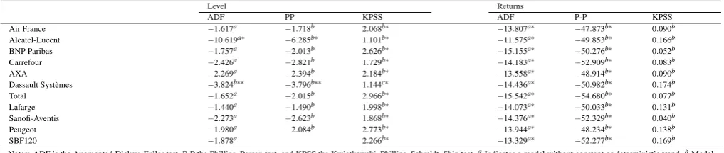
We study the stationarity properties of the series by performing three standard unit root tests: Augmented Dickey-Fuller (ADF), Phillips-Perron (P-P), and Kwiatkowski et al. (KPSS) tests. The ADF and P-P tests are based on the null hypothesis of a unit root, while KPSS test considers the null of no unit root. The obtained results in Table 5.3 shows that all of the return series are stationary at 1% significance level.

Table 5.2 summarizes selected basic statistics and correlation matrix for return series. On average, theTotalstock price experienced higher returns than all others stocks. SBF 120 stock market index has the smallest standard deviation. This shows that all stocks used in our study have higher volatility than SBF 120 stock market index. Skewness is positive in most cases and the Jarque-Bera test statistic (JB) strongly rejects the hypothesis of normality.

Air France

Date

Closing pr

ice

0 500 1000 1500 2000 2500

10 15 20 25 30 35

Dassault−Systèmes

Date

Closing pr

ice

0 500 1000 1500 2000 2500

20 30 40 50 60 70

Alcatel−Lucent

Date

Closing pr

ice

0 500 1000 1500 2000 2500

0 10 20 30 40 50 60 70

Total

Date

Closing pr

ice

0 500 1000 1500 2000 2500

30 35 40 45 50 55 60

BNP Paribas

Date

Closing pr

ice

0 500 1000 1500 2000 2500

20 30 40 50 60 70 80 90

Lafarge

Date

Closing pr

ice

0 500 1000 1500 2000 2500

40 60 80 100 120

Carrefour

Date

Closing pr

ice

0 500 1000 1500 2000 2500

30 40 50 60 70

Sanofi−Aventis

Date

Closing pr

ice

0 500 1000 1500 2000 2500

40 50 60 70 80

AXA

Date

Closing pr

ice

0 500 1000 1500 2000 2500

5 10 15 20 25 30 35

Peugeot

Date

Closing pr

ice

0 500 1000 1500 2000 2500

10 20 30 40 50 60

Air France

Date

Retur

n

0 500 1000 1500 2000 2500

−0.2 −0.1 0.0 0.1

Dassault−Systèmes

Date

Retur

n

0 500 1000 1500 2000 2500

−0.2 −0.1 0.0 0.1

Alcatel−Lucent

Date

Retur

n

0 500 1000 1500 2000 2500

−0.2 −0.1 0.0 0.1 0.2 0.3

Total

Date

Retur

n

0 500 1000 1500 2000 2500

−0.10 −0.05 0.00 0.05 0.10

BNP Paribas

Date

Retur

n

0 500 1000 1500 2000 2500

−0.2 −0.1 0.0 0.1 0.2

Lafarge

Date

Retur

n

0 500 1000 1500 2000 2500

−0.10 −0.05 0.00 0.05 0.10 0.15

Carrefour

Date

Retur

n

0 500 1000 1500 2000 2500

−0.10 −0.05 0.00 0.05 0.10

Sanofi−Aventis

Date

Retur

n

0 500 1000 1500 2000 2500

−0.10 −0.05 0.00 0.05 0.10

AXA

Date

Retur

n

0 500 1000 1500 2000 2500

−0.2 −0.1 0.0 0.1 0.2

Peugeot

Date

Retur

n

0 500 1000 1500 2000 2500

−0.15 −0.10 −0.05 0.00 0.05 0.10

Table 5.3

Unit root tests of time series.

Level Returns

ADF PP KPSS ADF P-P KPSS Air France −1.617a _−1.718b _2.068b∗ _−13.807a∗ _−47.873b∗ _0.090b Alcatel-Lucent −10.619a∗ −6.285b∗ 1.101b∗ −11.575a∗ −49.853b∗ 0.166b BNP Paribas −1.757a _−2.013b _2.626b∗ _−15.155a∗ _−50.276b∗ _0.052b Carrefour −2.426a _−2.821b _1.729b∗ _−14.183a∗ _−52.909b∗ _0.083b AXA −2.269a _−2.394b _2.184b∗ _−13.558a∗ _−48.914b∗ _0.090b Dassault Systèmes −3.824b∗∗ _−3.796b∗∗ _1.144c∗ _−14.436a∗ _−50.982b∗ _0.174b Total −1.652a _−2.015b _2.966b∗ _−15.542a∗ _−54.680b∗ _0.077b Lafarge −1.440a −1.490b 1.998b∗ −14.073a∗ −50.033b∗ 0.131b Sanofi-Aventis −2.273a _−2.623b _1.868b∗ _−14.376a∗ _−52.329b∗ _0.040b Peugeot −1.980a _−2.084b _2.773b∗ _−13.944a∗ _−48.234b∗ _0.138b SBF120 −1.878a _2.266b∗ _−13.329a∗ _−52.277b∗ _0.169b Notes: ADF is the Augmented Dickey–Fuller test, P-P the Phillips–Perron test, and KPSS the Kwiatkowski–Phillips–Schmidt–Shin test.a_{Indicates a model without constant or deterministic trend.}b_Model with constant and deterministic trend.∗Denotes rejection of the null hypothesis at the 1% level.∗∗Denotes rejection of the null hypothesis at the 5% level.∗∗∗Denotes rejection of the null hypothesis at the 10%level.

5.2 Empirical results

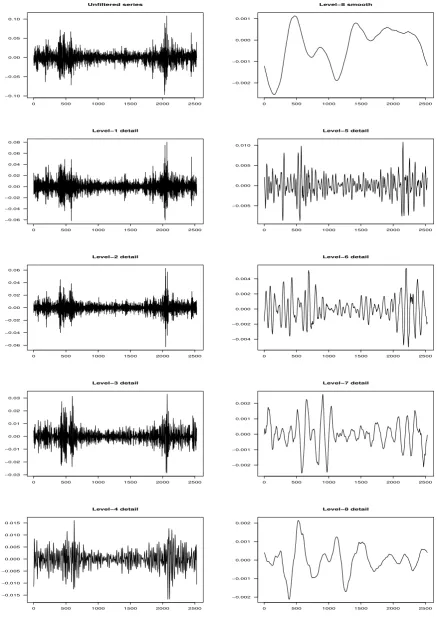
Firstly, we decomposed the return series into their time-scale components using MODWT. The filter used in the de-composition is the Daubechies least asymmetric (LA) wavelet filter of lengthL=8, or LA(8) wavelet filter, while our decomposition goes to scale 8 (scaleJ≤log₂N, N is the length of the time series). The LA(8) wavelet decomposition of daily returns for SBF 120 and weighted portfolio are shown in Figures 5.3 and 5.4. We plotted the returns of SBF 120 index and the weighted portfolio constructed from the ten assets and their corresponding details and smooths. We used daily data, the first level detailD1represents the variations within two days or four, while the next level details D2-D8represent the variations within 2jdays horizon (see Table 5.4 for explanation).

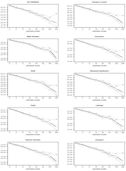
We performed a wavelet variance analysis on a scale-by-scale basis, thus we plotted the wavelet variance coefficients against scalesλj, j=1, . . . ,8 and we determine which scale contributes more in the variance of the process.9

As we can see in Figure 5.5, all stock returns show similar movements of wavelet variance. We can observe an approx-imate linear relationship between the wavelet variance and the wavelet scale. The variance of stock returns decreases as the wavelet scale increases, indicating that stock return variances are high in short terms (high frequencies) and low in long terms (low frequencies). As shown inKim and In(2005), the decrease in wavelet variance implies that an investor with a short investment horizon has to respond to every fluctuation in realized returns, while for an investor with a much longer horizon, the long run risk is significantly less.

To show the degree of association between stock market index and the constructed portfolio across scales, we focused in cross-correlation analysis.10 Hence, the cross-correlation function provides the degree of relationship between two time series as a function of time lag (h). This function measures the linear synchronization between the stock mar-ket index and the portfolio construced from the ten chosen assets. The results of wavelet cross-correlation between stock market index and our portfolio are reported in Figure 5.6. We observed that the first two scales, associated with periods of 2-4 days and approximately one week, indicate only a small number of lags (mostly arround zero) where the wavelet cross-correlation is different from zero (for scale 1 and for lags -1, 0 and 1 the values are -0.556, 0.920 and -0.515, respectively). We observed also that the wavelet cross-correlation appear to be roughly symmetric about zero lag from scale 1 up to scale 4. The asymmetry of cross-correlation function between stock market index and the portfolio becomes more pronounced as the scale increases. For instance, for scale 3 the values are 0.060 and 0.086 for lags -15 and 15, respectively, and for scale 5 the values are -0.436 and -0.515 for the same lags. On scales 6, 7 and 8 the symmetry disappear completely and we observed a positive correlation at scale 7 and scale 8 (128-256 days and 256-512 days). This indicates that when we are dealing with long run (more than two months), the prices of the

9_{The confidence interval is based on a Chi-squared distribution, an approximate(1−α)confidence interval for the wavelet variance can} be defined as follows: hξσ˜2

x(λj)/Kξ,1−α 2,ξσ˜

2

x(λj)/Kξ,α 2 i

, whereξ is the degree of freedom,K_ξ,1−α 2 andKξ,

α

2 are lower and upperα/2 quantiles. For a detailed explanation on how to construct the confidence interval of wavelet variance, seeGençay et al.(2002).

10_{The wavelet cross-correlations are computed from the equation (2.13) and the confidence interval for the wavelet cross-correlation (see}

Gençay et al.(2002)) is defined as follows:

tanh

h ρˆXY,τ(λj)

±Φ−1_(1−ρ)/q_Nˆ j−3

portfolio are positively correlated with future prices of stock market index.

As a summary, the wavelet cross-correlation analysis between the given portfolio at different time scales shows that the links among stock market returns vary with wavelet scales, moreover wavelet cross-correlation values are low at the lowest scales and high at highest ones.

Table 5.4

Interpretation of time scales.

Scale Component Frequency resolution Scale 1 D1 2 - 4 days

Scale 2 D2 4 - 8 days: approximately one week Scale 3 D3 8 - 16 days: approximately tow weeks Scale 4 D4 16 - 32 days: approximately one month Scale 5 D5 32 - 64 days: approximately 2 months Scale 6 D6 64 - 128 days: approximately 4 months Scale 7 D7 128 - 256 days: approximately 1 year Scale 8 D8 256 - 512 days: approximately 2 years

Notes: The lowest level detailD1captures frequencies 1/4≤f≤1/2 (i.e. any oscillation with a period length of 2 to 4 days), and the highest level detailD8captures frequencies 1/512≤f≤1/256 (i.e. any oscillation with a period length of 256 to 512 days).

5.2.1 Systematic risk analysis

Lintner(1965) andSharpe(1963,1964) showed that in asset pricing model a company’s total risk consists of two types

of risk: Unsystematic risk (idyosincratic risk) and systematic risk. 11 In our study, we only based on the changes of systematic risk over time horizons. The systematic risk, as denoted byβi in the asset pricing model, is a measure

of the slope of the regression in equation (4.6). The estimated Beta is therefore the measurement of systematic risk and represents a proxy for the true Beta. The systematic risk can differ from period to period and can be changed depending upon the management of each company. Moreover, managerial decisions about investments and financing influence the performance of the firm. Thus, the Beta could provide investors and company managers with various implications about a firm’s financial and investment policies.

To show the instability of systematic risk over time, we measured the Beta of various stocks over different time horizons using MODWT wavelet filter.

Table 5.5 reports the results of estimating Beta coefficient andR2 goodness of fit coefficient for the equation (4.6). Hence, the estimated coefficientβi(λj), j=1, . . . ,8 measures the contribution of scaleλjmovements in stock market

index to assets. As shown in Table 5.5 all the Beta coefficients are positive, indicating the positive correlation between assets and stock market index. We observed also, that the market risk of some stocks such asAir France, AXA, Dassault-Systèmes, Total, Lafarge andPeugeot increases with scales. For instance, from scale 1 up to scale 6Air FranceandAXAsystematic risk increased from 0.957 to 1.708 and 1.624 to 1.943, respectively, and from 0.965 and 1.435 forDassault-Systèmesbetween scale 1 to scale 5.

We observed also, that the systematic risk of almost stocks and for the proposed portfolio are less than one for the 2-4 days time horizon (short term). This, indicating that the market movements have a reduced impact on assets which provides less risk than market index in short term dynamics.

Figure 5.7 depicts the systematic risk variations of the ten assets with time scales. We observed that Beta seem to slightly decrease from the lowest to the highest scale for some stocks (for instance,BNP Paribas,Total, Sanofi-Aventis andCarrefour firms) and seem to slightly increase between lowest and highest scale for some others (for instance,Alcatel-LucentandAir Francefirms). Generally, when looking the plots of Beta of stocks, we remark that the systematic risk change non-monotocally with time scale, implying the different trading strategies of traders. We observed that long-term traders are averse to risk; at scale 7,AXA,Sanofi-AventisandPeugeotstocks are interrested by long-term traders than short-term traders (these assets have the smallest Beta at scale 7). At scales 1 and 2, Air France and Alcatel-Lucent stocks are interrested by short-term traders (these assets have small Beta). Therefore, we can say that short-term traders are "amateur" of risk.

11_{The total risk of an asset or a portfolio is measured by the variance or standard deviation of stock return. The idyosincratic risk is the}

Unfiltered series

0 500 1000 1500 2000 2500

−0.10 −0.05 0.00 0.05 0.10

0 500 1000 1500 2000 2500

Level−8 smooth

−0.0020 −0.0015 −0.0010 −0.0005 0.0000 0.0005 0.0010

0 500 1000 1500 2000 2500

Level−1 detail

−0.05 0.00 0.05

0 500 1000 1500 2000 2500

Level−5 detail

−0.010 −0.005 0.000 0.005

0 500 1000 1500 2000 2500

Level−2 detail

−0.06 −0.04 −0.02 0.00 0.02 0.04 0.06

0 500 1000 1500 2000 2500

Level−6 detail

−0.004 −0.002 0.000 0.002 0.004

0 500 1000 1500 2000 2500

Level−3 detail

−0.02 −0.01 0.00 0.01 0.02 0.03

0 500 1000 1500 2000 2500

Level−7 detail

−0.002 −0.001 0.000 0.001 0.002

0 500 1000 1500 2000 2500

Level−4 detail

−0.015 −0.010 −0.005 0.000 0.005 0.010 0.015

0 500 1000 1500 2000 2500

Level−8 detail

−0.002 −0.001 0.000 0.001 0.002

Unfiltered series

0 500 1000 1500 2000 2500

−0.10 −0.05 0.00 0.05 0.10

0 500 1000 1500 2000 2500

Level−8 smooth

−0.002 −0.001 0.000 0.001

0 500 1000 1500 2000 2500

Level−1 detail

−0.06 −0.04 −0.02 0.00 0.02 0.04 0.06 0.08

0 500 1000 1500 2000 2500

Level−5 detail

−0.005 0.000 0.005 0.010

0 500 1000 1500 2000 2500

Level−2 detail

−0.06 −0.04 −0.02 0.00 0.02 0.04 0.06

0 500 1000 1500 2000 2500

Level−6 detail

−0.004 −0.002 0.000 0.002 0.004

0 500 1000 1500 2000 2500

Level−3 detail

−0.03 −0.02 −0.01 0.00 0.01 0.02 0.03

0 500 1000 1500 2000 2500

Level−7 detail

−0.002 −0.001 0.000 0.001 0.002

0 500 1000 1500 2000 2500

Level−4 detail

−0.015 −0.010 −0.005 0.000 0.005 0.010 0.015

0 500 1000 1500 2000 2500

Level−8 detail

−0.002 −0.001 0.000 0.001 0.002

* * * * * * * * 5e−04 1e−03 2e−03 5e−03 1e−02 2e−02 5e−02 1e−01 2e−01 Air FRANCE wavelet scale L L L L L L L L U U U U U U U U

2 4 8 16 32 64 128 256

* * * * * * * * 5e−04 1e−03 2e−03 5e−03 1e−02 2e−02 5e−02 1e−01 2e−01 5e−01 Alcatel−Lucent wavelet scale L L L L L L L L U U U U U U U U

2 4 8 16 32 64 128 256

* * * * * * * * 5e−05 1e−04 5e−04 1e−03 5e−03 1e−02 5e−02 1e−01 BNP Paribas wavelet scale L L L L L L L L U U U U U U U U

2 4 8 16 32 64 128 256

* * * * * * * * 1e−04 5e−04 1e−03 5e−03 1e−02 5e−02 1e−01 Carrefour wavelet scale L L L L L L L L U U U U U U U U

2 4 8 16 32 64 128 256

* * * * * * * * 2e−04 5e−04 1e−03 2e−03 5e−03 1e−02 2e−02 5e−02 1e−01 2e−01 5e−01 AXA wavelet scale L L L L L L L L U U U U U U U U

2 4 8 16 32 64 128 256

* * * * * * * * 2e−04 5e−04 1e−03 2e−03 5e−03 1e−02 2e−02 5e−02 1e−01 2e−01 Dassault Systèmes wavelet scale L L L L L L L L U U U U U U U U

2 4 8 16 32 64 128 256

* * * * * * * * 5e−05 1e−04 5e−04 1e−03 5e−03 1e−02 5e−02 1e−01 Total wavelet scale L L L L L L L L U U U U U U U U

2 4 8 16 32 64 128 256

* * * * * * * * 1e−04 5e−04 1e−03 5e−03 1e−02 5e−02 1e−01 Lafarge wavelet scale L L L L L L L L U U U U U U U U

2 4 8 16 32 64 128 256

* * * * * * * * 5e−05 1e−04 5e−04 1e−03 5e−03 1e−02 5e−02 1e−01 Sanofi−Aventis wavelet scale L L L L L L L L U U U U U U U U

2 4 8 16 32 64 128 256

* * * * * * * * 2e−04 5e−04 1e−03 2e−03 5e−03 1e−02 2e−02 5e−02 1e−01 2e−01 Peugeot wavelet scale L L L L L L L L U U U U U U U U

2 4 8 16 32 64 128 256

Level 8

−1.0

−0.5

0.0

0.5

1.0

−24 −12 0 12 24

Lag (days)

Level 7

−1.0

−0.5

0.0

0.5

1.0

−24 −12 0 12 24

Lag (days)

Level 6

−1.0

−0.5

0.0

0.5

1.0

−24 −12 0 12 24

Lag (days)

Level 5

−1.0

−0.5

0.0

0.5

1.0

−24 −12 0 12 24

Lag (days)

Level 4

−1.0

−0.5

0.0

0.5

1.0

−24 −12 0 12 24

Lag (days)

Level 3

−1.0

−0.5

0.0

0.5

1.0

−24 −12 0 12 24

Lag (days)

Level 2

−1.0

−0.5

0.0

0.5

1.0

−24 −12 0 12 24

Lag (days)

Level 1

−1.0

−0.5

0.0

0.5

1.0

−24 −12 0 12 24

Lag (days)

Figure 5.6 Wavelet cross-correlation between the SBF 120 and the Weighted portfolio returns. The individual

cross-correlation functions correspond to wavelet scalesλ1, . . . ,λ8(i.e. the correlation coefficient of the value of portfolio

Air France

wavelet scale

Beta

1 2 3 4 5 6 7 8

1.0 1.5 2.0 2.5

Alcatel−Lucent

wavelet scale

Beta

1 2 3 4 5 6 7 8

1.6 1.8 2.0 2.2 2.4

BNP Paribas

wavelet scale

Beta

1 2 3 4 5 6 7 8

0.4 0.6 0.8 1.0 1.2 1.4

Carrefour

wavelet scale

Beta

1 2 3 4 5 6 7 8

0.0 0.2 0.4 0.6 0.8

AXA

wavelet scale

Beta

1 2 3 4 5 6 7 8

1.4 1.6 1.8 2.0

Dassault Systèmes

wavelet scale

Beta

1 2 3 4 5 6 7 8

0.8 1.0 1.2 1.4

Total

wavelet scale

Beta

1 2 3 4 5 6 7 8

0.5 0.6 0.7 0.8 0.9

Lafarge

wavelet scale

Beta

1 2 3 4 5 6 7 8

0.4 0.6 0.8 1.0 1.2 1.4

Sanofi−Aventis

wavelet scale

Beta

1 2 3 4 5 6 7 8

0.4 0.5 0.6 0.7 0.8

Peugeot

wavelet scale

Beta

1 2 3 4 5 6 7 8

0.8 0.9 1.0 1.1 1.2

Figure 5.7 Betas of assets as a function of scale. The wavelet-Beta estimate for each stock i, at scaleλj, was computed as

ˆ

Table 5.5

Market model regression.

Air France

Alcatel-Lucent

BNP Paribas

Carrefour AXA Dassault-Systèmes

Total Lafarge Sanofi-Aventis

Peugeot Portfolio

Panel A: Unfiltered series

Beta 1.104 1.597 1.294 0.877 1.668 1.013 0.923 1.059 0.756 0.997 0.956

R2 0.373 0.469 0.619 0.491 0.719 0.365 0.632 0.503 0.380 0.430 0.842

Panel B: Beta

Scale 1 0.957 1.519 1.297 0.900 1.624 0.965 0.969 0.994 0.800 0.919 0.954 Scale 2 1.099 1.596 1.254 0.879 1.678 1.011 0.939 1.061 0.748 1.058 0.961 Scale 3 1.378 1.723 1.365 0.813 1.722 1.017 0.823 1.211 0.777 1.091 0.980 Scale 4 1.464 1.519 1.535 0.900 1.782 1.231 0.824 1.212 0.548 1.185 0.922 Scale 5 1.551 2.112 1.064 0.927 1.943 1.435 0.842 1.134 0.554 1.163 0.994 Scale 6 1.708 2.260 9.310 0.590 1.952 1.201 0.534 1.275 0.505 0.888 0.865 Scale 7 1.756 2.236 1.117 0.535 1.630 0.978 0.667 0.905 0.403 0.807 0.793 Scale 8 2.021 2.993 1.757 0.437 1.556 1.445 0.586 1.681 0.131 1.425 0.892

Panel C:R2

Scale 1 0.306 0.443 0.647 0.506 0.730 0.338 0.671 0.463 0.427 0.397 0.847 Scale 2 0.399 0.497 0.615 0.505 0.699 0.368 0.633 0.522 0.374 0.459 0.840 Scale 3 0.501 0.528 0.591 0.468 0.717 0.395 0.581 0.602 0.363 0.508 0.841 Scale 4 0.439 0.386 0.608 0.471 0.738 0.442 0.515 0.536 0.200 0.473 0.812 Scale 5 0.504 0.507 0.473 0.408 0.705 0.501 0.511 0.539 0.195 0.408 0.796 Scale 6 0.679 0.630 0.472 0.274 0.781 0.533 0.395 0.606 0.260 0.411 0.856 Scale 7 0.636 0.513 0.298 0.205 0.607 0.399 0.477 0.400 0.122 0.190 0.805 Scale 8 0.739 0.635 0.757 0.239 0.789 0.457 0.574 0.602 0.018 0.521 0.894

5.2.2 VaR analysis

After analyzing market risk by estimating the Beta coefficients from regression in equation (4.4), we will measure the market risk of the ten stocks and the portfolio constructed from these stocks by computing the VaR at different time scales. The results are reported in table 5.6 and table 5.7. We computed the contribution to VaR (column 5 in table 5.7) of the portfolio constructed from the ten stocks using the measure:

ˆ

σ2 m(λj)

∑N_i=1κiβˆi(λj) 2

+∑N_i=1κ2 i σˆεi2(λj)

ˆ

σ2 m

∑N_i=1κiβˆi 2

+∑N_i=1κ2 iσˆεi2

(5.1)

ˆ

σ2

εi(λj)are given by

ˆ

σ_εi2(λj) =σˆi2(λj)−βˆi2(λj)σˆm2(λj),i=1, . . . ,N; j=1, . . . ,J (5.2)

In Figure 5.8 we depicted Value at Risk of all stock returns and of the weighted diversified portfolio. We observed that all VaRs decrease monotocally from low scale (high frequency dynamics) to high scales (low frequency dynamics). This, indicates that market risk is concentrated at the lower scale of the data (short term dynamics).

6

Extension: Performance measurement

This section extends the analysis to the performance evaluation of a portfolio. There are more measures of perfor-mance such asSortino ratio(Sortino and Meer(1991)), the Treynor ratio(Treynor(1961)),Farinelli-Tibiletti ratio

(Tibiletti and Farinelli(2003)),Sharpe ratio(Sharpe(1964)) and others. In our analysis we focused inSharpe ratio.

This ratio is widely used and is the best known performance measure in the investment strategies. For comparison purposes, we considered both traditionalSharpe ratioand modifiedSharpe ratio. The traditional approach is defined as follows: Suppose we have a portfolio with returnRport f olioand observe a benchmark portfolio (market index) with

a returnRbenchmark, then the traditionalSarpe ratiois

SRTraditional=

Rport f olio−Rbenchmark σport f olio

●

●

●

●

●

●

●

● ●

●

●

●

●

●

●

● ●

●

Air France Alcatel−Lucent BNP Paribas Carrefour AXA

Dessault Systèmes Total

Lafarge Sanofi−Aventis Peugeot Portfolio

1 2 3 4 5 6 7 8

0.00 0.01 0.02 0.03 0.04

wavelet scale

Value at Risk

Figure 5.8 Individual VaR and diversified VaR (weighted portfolio constructed from ten stocks of firms) at different time scales. VaR were computed at the 95% significance level.

whereσport f oliois the standard deviation of portfolio over a sample period. The modified Sharpe ratio is given by

SRmodi f ied=

Rport f olio−Rbenchmark

VaRport f olio

(6.2)

whereVaRport f oliois the VaR of a given portfolio.

Using wavelet analysis, we computed theSharpe ratioat different time scales.

SRmodi f iedandSRTraditionalare all negative, indicating that the portfolio constructed from various ten stocks

underper-formed the market index during scales.

7

Concluding remarks

Using wavelets we examined the dynamics of stock returns of 10 firms from Paris Stock Market during the period between December 29, 2000 and September 06, 2010. The MODWT was applied to decompose the daily returns into multiscale components. Firstly, we provide a multiscale decomposition of the variance and the correlation to identify the time-frequency properties of the stock returns. Wavelet variance analysis shows that all stocks exhibit a long memory behavior, i.e. we observed an approximate linear relationship between the wavelet variance and the wavelet scale, with a slow decreasing in the wavelet variance as the wavelet scale increases. Wavelet cross-correlation analysis is used to measure the degree of association (the dynamic linking) between stocks returns among scales. The results show that at low scales the relationship between stock returns is generally close to zero, while at high scales, the association become stronger. Our findings are consistent with some recent studies, such as, the study ofGallegati

(2005) on examining the features of stock returns and aggregate economic activity, the studies ofKim and In(2005,

Table 5.6

Value at Risk at different time scales.

Air France Alcatel-Lucent BNP Paribas Carrefour AXA VaR Contribution to

VaR (%)

VaR Contribution to VaR (%)

VaR Contribution to VaR (%)

VaR Contribution to VaR (%)

VaR Contribution to VaR (%) Scale 1 0.0308 33.60 0.0407 49.38 0.0287 49.51 0.0225 52.75 0.0339 48.17 Scale 2 0.0222 24.43 0.0287 24.54 0.0203 24.78 0.0156 25.38 0.0256 27.44 Scale 3 0.0169 14.28 0.0207 12.81 0.0155 14.46 0.0103 11.12 0.0178 13.29 Scale 4 0.0124 7.69 0.0137 5.64 0.0110 7.28 0.0072 5.48 0.0116 5.67 Scale 5 0.0081 3.32 0.0110 3.65 0.0057 1.98 0.0053 3.01 0.0087 3.21 Scale 6 0.0057 1.61 0.0080 1.93 0.0038 0.89 0.0031 1.04 0.0062 1.64 Scale 7 0.0031 0.49 0.0044 0.59 0.0029 0.51 0.0019 0.39 0.0025 0.27 Scale 8 0.0022 0.25 0.0017 0.09 0.0005 0.01 0.0009 0.10 0.0010 0.05 Recomposed data 0.0449 0.0579 0.0409 0.0310 0.0489 Raw data 0.0449 0.0579 0.0409 0.0310 0.0489 Dassault Systèmes Total Lafarge Sanofi-Aventis Peugeot VaR Contribution to

VaR (%)

VaR Contribution to VaR (%)

VaR Contribution to VaR (%)

VaR Contribution to VaR (%)

VaR Contribution to VaR (%) Scale 1 0.0296 50.63 0.0211 53.69 0.0260 49.49 0.0218 51.37 0.0260 47.48 Scale 2 0.0210 25.66 0.0150 27.13 0.0186 25.38 0.0155 26.12 0.0198 27.70 Scale 3 0.0140 11.38 0.0093 10.57 0.0136 13.51 0.0112 13.63 0.0133 12.46 Scale 4 0.0104 6.32 0.0063 4.91 0.0092 6.23 0.0067 4.87 0.0096 6.57 Scale 5 0.0076 3.35 0.0044 2.34 0.0054 2.18 0.0044 2.09 0.0066 3.11 Scale 6 0.0041 1.01 0.0024 0.72 0.0048 1.68 0.0029 0.95 0.0037 0.97 Scale 7 0.0022 0.29 0.0016 0.31 0.0021 0.34 0.0019 0.39 0.0027 0.51 Scale 8 0.0012 0.08 0.0007 0.06 0.0008 0.05 0.0006 0.04 0.0012 0.10 Recomposed data 0.0416 0.0288 0.0370 0.0305 0.0377 Raw data 0.0416 0.0288 0.0370 0.0305 0.0377 Notes: The contribution to VaR is computed as the ratio of stock returns variances. We computed the wavelet variance using equation (2.7) and we divided them by the total variance.

Table 5.7

VaR at different time scales for weighted portfolio and market index.

SBF120 (α=5%) portfolio (α=5%)

VaR Contribution to VaR (%) VaR Contribution to VaR (%) Scale 1 0.0178 51.61 0.0105 51.03

Scale 2 0.0127 26.25 0.0075 26.70 Scale 3 0.0087 12.36 0.0052 13.02 Scale 4 0.0055 5.03 0.0034 4.85 Scale 5 0.0037 2.23 0.0024 2.54 Scale 6 0.0026 1.17 0.0016 1.00 Scale 7 0.0014 0.35 0.0009 0.24 Scale 8 0.0005 0.05 0.0004 0.03 Recomposed data 0.0248 0.0259

Raw data 0.0248 0.0259

Notes: The VaR of SBF 120 stock market index is computed asVaR(λj) =σm(λj)F−1(), whereσm(λj)is the standard deviation of stock market index return at scaleλjandF−1()is the quantile of the inverse normal cumulative distribution. The VaR of the portfolio is computed using the equation (4.12). The contribution to VaR computed for SBF 120 is the ratio between wavelet variance and the total variance, and the contribution to VaR of the portfolio (column 5) is computed using the equation (5.1).

on VaR. The results showed that the risk (measured by VaR) is concentrated more at higher frequencies (lower scales). These results are consistent with the results ofGençay et al.(2005),He et al.(2009) andMasih et al.(2010).

References

Coifman, R. R., Donoho, D. L., 1995. Translation-invariant de-noising. Lecture Notes in Statistics: Wavelet and Statistics, 125–150.

Daubechies, I., 1992. Ten lectures on wavelets. Society for Industrial and Applied Mathematics, Philadelphia, PA, USA.

Durai, S. R. S., Bhaduri, S. N., 2009. Stock prices, inflation and output: Evidence from wavelet analysis. Economic Modelling 26 (5), 1089 – 1092.

Fernandez, V., 2006. The capm and value at risk at different time-scales. International Review of Financial Analysis 15 (3), 203–219.

Table 6.1

Comparisons of the traditional and modified ratios.

Modified Sharpe ratio Traditional Sharpe ratio Scale 1 -0.0140 -0.0011

Scale 2 -0.0139 -0.0022 Scale 3 -0.0199 -0.0046 Scale 4 -0.0306 -0.0124 Scale 5 -0.0433 -0.0236 Scale 6 -0.0655 -0.0598 Scale 7 -0.1082 -0.2412 Scale 8 -0.2608 -1.5540 Unfiltered series -0.0057 -0.6017

Gençay, R., Selçuk, F., Whitcher, B., 2002. In: An Introduction to Wavelets and Other Filtering Methods in Finance and Economics. Academic-Press.

Gençay, R., Selçuk, F., Whitcher, B., 2005. Multiscale systematic risk. Journal of International Money and Finance 24 (1), 55–70.

He, K., Xie, C., Chen, S., Lai, K. K., 2009. Estimating var in crude oil market: A novel multi-scale non-linear ensemble approach incorporating wavelet analysis and neural network. Neurocomputing 72 (16-18), 3428 – 3438.

Heni, B., Boutahar, M., 2011. A wavelet-based approach for modelling exchange rates. Statistical Methods and Ap-plications 20, 201–220.

In, F. H., Kim, S., 2006. Multiscale hedge ratio between the australian stock and futures markets: Evidence from wavelet analysis. Journal of Multinational Financial Management 16 (4), 411 – 423.

Jorion, P., 1996. In: Risk and Turnover in the Foreign Exchange Market. National Bureau of Economic Research, Inc.

Kim, S., In, F., 2007. On the relationship between changes in stock prices and bond yields in the g7 countries: Wavelet analysis. Journal of International Financial Markets, Institutions and Money 17 (2), 167–179.

Kim, S., In, F. H., 2005. The relationship between stock returns and inflation: new evidence from wavelet analysis. Journal of Empirical Finance 12 (3), 435–444.

Lintner, J., 1965. The valuation of risk assets and the selection of risky investments in stock portfolios and capital budgets. The Review of Economics and Statistics 47 (1), 13–37.

Mallat, S. G., 1989. A theory for multiresolution signal decomposition: The wavelet representation. IEEE Transac-tions on Pattern Analysis and Machine Intelligence 11, 674–693.

Masih, M., Alzahrani, M., Al Titi, O., 2010. Systematic risk and time scales: New evidence from an application of wavelet approach to the emerging gulf stock markets. International Review of Financial Analysis 19 (1), 10–18.

Mondal, D., Percival, D. B., 1995. On estimation of the wavelet variance. Biometrika 82, 619–631.

Nason, G. P., Silverman, B. W., 1995. The stationary wavelet transform and some statistical applications. Springer-Verlag, pp. 281–300.

Norsworthy, J. R., Li, D., Gorener, R., 2000. Wavelet-based analysis of time series: an export from engineering to finance. IEEE Engineering Management Society 2, 126 – 132.

Percival, D. B., 1995. On estimation of the wavelet variance. Biometrika 82, 619–631.

Percival, D. B., Guttorp, P., 1994. Long-memory processes, the allan variance and wavelets. Wavelets in geophysics.

Percival, D. B., Walden, A. T., 2000. Wavelet methods for time series analysis. Cambridge University Press.

Pesquet, J. C., Krim, H., Carfantan, H., 1996. Time invariant orthonormal wavelet representations. IEEE transactions on signal processing 44, 1964–1970.

Ramsey, J. B., Zhang, Z., 1997. The analysis of foreign exchange data using waveform dictionaries. Journal of Em-pirical Finance 4 (4), 341–372.

Sharkasi, A., Crane, M., Ruskin, H. J., Matos, J. A., 2006. The reaction of stock markets to crashes and events: A com-parison study between emerging and mature markets using wavelet transforms. Physica A: Statistical Mechanics and its Applications 368 (2), 511 – 521.

Sharpe, W. F., 1963. A simplified model for portfolio analysis. Journal of Financial and Quantitative Analysis 09 (02), 277–293.

Sharpe, W. F., 1964. Capital asset prices: A theory of market equilibrium under conditions of risk. Journal of Finance 19, 425–442.

Sortino, F. A., Meer, R. v. d., 1991. Downside risk. The Journal of Portfolio Management 17 (4), 27–31.

Tibiletti, L., Farinelli, S., 2003. Upside and downside risk with a benchmark. Atlantic Economic Journal 31 (4), 387–387.

Treynor, J. L., 1961. Market value, time, and risk. Unpublished manuscript.