A Dynamic Optimization on Energy
Efficiency in Developing Countries
Wang, Dong
24 November 2012
A Dynamic Optimization on Energy Efficiency in Developing
Countries
Dong Wang
Crawford School of Public Policy, Australian National University, Canberra, Australia
Business School of Sichuan University, Chengdu, China
Email: [email protected]
ABSTRACT
This paper introduces a way for measuring the energy efficiency in economics besides
the methods in physics. The linkage among energy efficiency, energy consumption and
other macroeconomic variables is demonstrated primarily. Based on the methodology of
dynamic optimization, a maximum problem of energy efficiency over time is subjected
to the extended Solow growth model and instantaneous investment rate. In this model,
energy consumption is set as control variable and investment is regarded as state
variable. The analytic solutions can be derived and the diagrammatic analysis provides
saddle-point equilibrium. With assigning values to parameters, a numerical simulation is
presented; meanwhile the optimal paths of investment and energy consumption can be
drawn. The discussion on modelling and implications is organized in the end. The
dynamic optimization encourages governments in developing countries to pursue higher
energy efficiency as it can reduce energy use without influencing the achievement of
steady state in terms of Solow model.
1
Introduction
Social planners and policymakers have been attracted by dynamic optimization issues
for many years. To some degree, ‘path choice problem’always lies in the centre of policy debate not only in developed countries, but especially in developing countries.
Although a large quantity of researches have discussed on the optimal path of economic
growth, energy consumption or pollution reduction, seldom economists have set their
feet in the energy efficiency issues under the view of dynamic. In fact, the improvement
of energy efficiency is a dynamic procedure in the development and it is always related
to growth, investment, technology change and many other economic variables.
Energy efficiency can be defined in three dimensions. The first definition stems from
the laws of thermodynamics in physics. It is defined as a ratio of best practice energy
input over energy input, ceteris paribus, which refers to technical efficiency1 (Jin &
Arons, 2009) and cannot be greater than one. The second definition is based on
economic concepts and named energy intensity2, which is the ratio of energy input over
output (National Bureau of Statistics of China, 2010). However, this definition only
considers energy as a unique input with ignoring the other factors in the production such
as capital and labour. David Stern (2012) has developed this definition of economic
energy efficiency under the multi-input framework. In his work, the economic technical
efficiency is on the basis of Pareto principle and is associated with capital as another
input. He stated that any economy has two inputs for production. The one is energy and
the other is capital. People should utilize the input composition to attain the goal of
output and growth. Thus, by this argument, there must be an optimal solution about the
input combination in development, which can be seen as the economic energy efficiency.
The things people need to do are to make the economy operating under the best energy
efficiency condition. In this paper, I adapt the meaning of energy efficiency is based on
the Stern’s definition. In other words, I consider how to allocate and utilize energy and
1
The thermodynamic definition of the energy efficiencyηis η = 𝑊𝑖𝑛𝑚𝑖𝑛
𝑊𝑖𝑛𝑟𝑒𝑎𝑙≤ 1
2 energy intensity =𝐸
capital as two inputs efficiently for achieving the desired output and growth.
The attendant question is why the economic energy efficiency is crucial? In many
developing countries, it is inevitable that the energy consumption is increasing with a
rapid economic growth and the improvement of living standards. This may lead to
energy security and environmental problems meanwhile. Probably, a continuous
increase in energy efficiency is an appropriate solution for this dilemma, even though
energy efficiency cannot be increased infinitely in terms of the second law of
thermodynamics.
Apparently, advanced technology applications can increase energy efficiency. Besides
that, the underlying drivers are capital, human resources and even energy itself. Firstly,
investment and skilled labour can promote technology and energy utilization; secondly,
different types of energy have different potential for energy efficiency promotion. The
modern energy contains more exergy3, meaning that higher energy efficiency could be
achieved. However, the transition from conventional energy to modern energy in
developing countries also needs sufficient capital accumulation and adequate economic
growth. Hence, the improvement of energy efficiency is interlinked with investment
capacity, labour force quality and economic growth stages.
Nonetheless, the labour force shifts spontaneously and cannot be controlled or planned
easily. While the investment whether in its scale or speed, is controllable in most
situations. Additionally, investment can influence the improvement of energy efficiency
by means of technology and furthermore, influence the energy consumption and
economic growth. That is to say, the pace of energy efficiency improvement should
feature dynamic and be restricted by capital, growth and energy itself. Consequently,
there may be a dynamic optimal path of energy efficiency improvement in development.
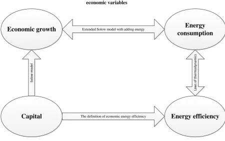
The mechanism is illustrated as Figure 1.
3
It is of importance and inspiration on both theory and practice. In theory, if we can
model the dynamic path of energy efficiency linking with energy consumption and
economic growth, we can introduce energy efficiency into traditional
‘energy-economy-environment’ (3E) analysis. Furthermore, the coming 3E analysis on
technology transformation, factor allocation and energy transition could access to
energy efficiency discussion. In practice, the modelling could reveal the best choice of
controlled path for developing countries on how to enhance energy efficiency given the
limited capital stock and investment.
The purpose of this paper is to model the dynamic optimal path of energy efficiency
improvement given the investment shift and production function. Firstly, a function is
established for measuring energy. Secondly, Solow growth is extended by adding energy
and deriving the instantaneous state equation of investment. Lastly, the steady-state
solution can be solved by dynamic optimization method. The paper is organised by six
parts. The literature review follows the introduction, and then the methodology is
introduced in section three. Results and a numerical simulation are presented in section
Economic growth Energy
consumption
Capital Energy efficiency
Extended Solow model with adding energy
S o lo w m o d e l L aw s o f th e rm o d y n am ic s
[image:5.595.99.550.104.386.2]The definition of economic energy efficiency
four followed by some discussions in section five. The conclusion is arranged at the end
of the paper.
2
Literature review
The reviewed literature includes three categories: the application of dynamic
optimization in exhaustible resource economics; the recent work on the dynamic
relationship among energy, economy and environment; and the literature on energy
efficiency.
Dynamic optimization has been applied for resource exploration problems since 1970s
(Pindyck, 1978, 1980). He established a basic model on the optimal exploration of
non-renewable resources in 1978 and developed it in 1980 with adding uncertainty into
exhaustible resource market analysis. Both of the two models are based on cost benefit
analysis. Basically, they are general models and they only focus on the optimization in
production. The shortcoming is that the energy depletion in the models has not been
linked with economic growth and any other macroeconomic variables.
Some other economists (Stiglitz, 1974; Garg and Sweeney, 1978; Dasgupta and Heal,
1979) brought the optimal exploration problem into the framework of neoclassical
model of growth. They have discussed well on the optimal sustainable growth path
under the condition that the resources are scarcity and diminishing all the time. But the
technology element was assumed exogenous in their models, which has aroused a wide
controversy. Having the endogenous growth model been raised (Romer, 1990; Lucas,
1988), the technology change became endogenous so that the long-run analysis was
feasible and reasonable. Nevertheless, the literature on endogenous growth model rarely
includes the natural resources problems. The two recent papers for China’s issues are
written by Peng (2007) and Li et al. (2012). They developed the endogenous growth
model with treating natural resources as a constraint and got an optimal path of
development eventually. But they do not mention the issues about energy efficiency.
issues from dynamic perspective. The most famous example is Forster model which was
raised in 1980. The model constructed an instantaneous utility function which depends
on the level of consumption and pollution by means of the principle of utility theory.
Since the pollution can be associated with energy use in Forster model, we can establish
a maximum problem with energy as a control variable. It is a regular model for
considering the optimization problem in energy and environmental fields. In addition,
Chiang provided a similar optimal example about anti-pollution policy (1992). Besides,
Conrad (2001) linked energy with carbon emission and solved an optimal path for
resource allocation. These researches provide a thinking direction on energy and
environment, and inspire me somehow. But they do not discuss the energy efficiency
either.
On the side of energy efficiency, the papers, usually, are case by case instead of
providing a general and theoretical framework. Moreover, most of the discussions are
on the technology level with using the technical definition not economic definition of
energy efficiency. For instance, Jaffe and Stavins (1994) stated the five dimentions of
optimal energy use for analying the energy-efficiency gap; two recent papers on energy
efficiency are on the level of technology applications and management (Sanchez & Ruiz,
2009; Brennan, 2010). Although Stern (2012) models the international trends of energy
efficiency detailedly, his work does not involve the dynamic improvement path issue.
Thus, a generalised analysis on the optimal energy efficiency path from economics
perspective is needed.
3
Methodology
The optimal energy efficiency path is hard to discover mainly because the energy
efficiency is hard to be defined apporprately. In this section, the modelling will start
with a quantative definition which is given by mathmatical and geometrical method.
And then, Solow model will be extended with taking energy consumption into account.
After these preparations, the dynamic maximum problem with constraints will be
3.1The meaning of economic energy efficiency
The economic energy efficiency can be defined as a function of capital stock and energy
consumption under the multi-input framework. Obviously, energy efficiency depends on
energy use. The reasons that we encompass capital in the model are from the views of
stock and flow angles. For one thing, the level of capital stock determines the level of
development and technology, which is the foundation in energy efficiency improvement.
For another thing, the capital flow is directly associated with investment, which is the
key driver of economic growth and technology progress in developing countries. Thus,
capital is tightly related with the energy efficiency. In this model, technology is assumed
exogenous and it is embodied by investment and capital stock level.
With the energy and capital as two inputs, to some extent, economic energy efficiency is
similar to production function. On the other hand, some certain level of energy
efficiency can be evaluated and compared with each other, similar to the methods used
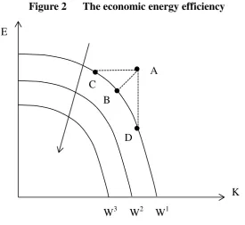
[image:8.595.183.459.444.696.2]in the theory of ordinal utility. This definition is demonstrated geometrically in Figure 2.
Figure 2 The economic energy efficiency
In figure 2, the three curves represent three levels of energy efficiency under different
technology, capital, energy consumption or output conditions. All points on the curves
are efficient states. The direction of the arrow means energy efficiency increasing,
E
K A
B C
D
implying that ‘the less, the better’ for inputs. Given the level of output, the less inputs
use means the more efficient energy economic system is. W stands for energy efficiency,
as a result, 𝑊3 > 𝑊2 > 𝑊1.
The energy efficiency curve is concave rather than curving inward mainly because of
diminishing marginal rate of substitution. That is how much capital input increase can
substitute one unit of energy we reduce. It is similar to the production-possibility curve.
There are two ways for increasing energy efficiency, which are demonstrated by both
arrow and dotted line. A is on the right of curve W1, meaning that A use more energy
and capital than the system indeed need given the best efficient curve W1. So A is
inefficient point. B, C and D on W1 are all the efficient points. Now, we have three paths
to haul the inefficient point A back to the efficient state W1
,
which is called diminishingthe energy distance. If we reduce both energy and capital, we can get B; if we only
reduce energy with holding capital input unchanged, we can get D; if we only reduce
capital with holding energy input unchanged, we can get C.
Another important thing is about other macroeconomic variables change including
technology, investment and output. For any certain output, technology progress can
improve the best level of efficiency (the curves). Put differently, the state shift from W1
to W3 may result from technology advance which is associated with the level of capital.
In this situation, we call the economy climbing the energy efficiency curves. Modelling
in this paper is indicating this situation instead of energy distance.
An equation for quantifying the level of energy efficiency W is
( ) = 2 > (1)
Where W is the level of energy efficiency; K is capital input and E is Energy input. α is
3.2The extended Solow model
For linking energy with growth and investment, we should extend neoclassical growth
model. Holding technology as an exogenous variable, Stern (2011) developed the Solow
model and discussed the role of energy in growth. However, his model is so
complicated that it cannot be solved. In this paper, I provide a simple extended model as
follow.
= (1 ) 1 1 1 ( )
Equation (2) embeds Solow model, which is a Cobb-Douglas function of value added,
with adding energy (E), which produces gross output Y. The term of 1 is the
traditional component of Solow model with capital (K) and labour (L). β and γ are
parameters. γ reflects the relative importance of energy and Solow value added.
Besides, we can get an equation on instantaneous investment state which reveals capital
flow.
̇ = ( ) 1 1 ( )
Here, ̇ is the growth rate of the capital stock which refers to investment. s is the rate
of saving. The capital depreciates at a constant rate δ. The term ( ) is different
from Solow model. It implies that, under the energy constraint, the true accumulated
capital should be adjusted by energy consumption. Hence, the instantaneous increment
of capital is the proportion of gross output with subtracting the depreciation of capital
stock from the net accumulative capital.
3.3The maximum dynamic problem
Modelling on the maximum dynamic problem of energy efficiency under the growth
∫ 𝑊( ) ( )
s. t. = (1 ) 1 ( )
̇ = ( ) ( )
( ) = ( )
The equation (2) and (3) are two constraints and equation (3) is state equation.
Accordingly, capital (K) is the state variable and energy (E) is the control variable. The
equation (4) does not include discounting rate in terms of the specific problem of energy
efficiency. As mentioned above, the main meaning of the function (1) is for indicating
the degree of energy efficiency and for comparing different levels of efficiency. Thus, it
has little meaning in discounting.
Concerning about the boundary condition, the initial value of the state variable is given
by E0, and the terminal value is free. T is the ending time and it is flexible or . In
this free ending point problem, the transversality condition is
( ) = ( ) = ( )
Substituting equation (2) into (3) and integrating them as one constraint, the
Hamiltonian is given by
= ( ) [s( ) ]
= 2 [s ((1 ) 1 ) ] ( )
The first order condition is
̇ = ( )
̇ = ( ) ( )
4
Results
4.1Diagrammatic analysis
I use phrase-diagram to analyze the steady-state of this constrained problem. Suppose
that labour is constant, denoting ̅. That is, during the observed years, the gross number
of the labour force in the country should not change. Solving for the steady-state point,
the first order condition can be rewritten as
= = (1 )
̇ = 𝜕𝐻
𝜕𝐾= (1 ) ̅1 1 (11)
̇ = [(1 ) 1 ] = (1 )
From equation (10), we can get
= ( 1) (1 )
The derivative of E is
̇ = ( 1) ̇ (1 )
Substitute equation (11) into (14),
̇ =( 1) ̇ =( 1)[ (1 ) ̅1 1 ] = (1 )
= [ (1 ) ̅ 1 ]
1 1
( ̇ = curve ) (1 )
Equation (16) is for ̇ = curve. It only depends on the parameters of the system and
the scale of population. This is a constant in the E—K space as illustrated in Figure 3.
Solving equation (12), we can get the solution is
=
(1 ) ̅1 ( ̇ = curve ) (1 )
Equation (17) is for ̇ = curve as illustrated in Figure 3. Consequently, the
differential system of E and K in E—K space is
̇ =( 1)( ) ( 1) (1 ) ̅1 1 (1 )
̇ = ( 1) (1 ) ̅1 (1 )
The direction of movement depends on the signs of the derivatives ̇ and ̇ at
particular point in the E—K space. We can find by the differentiation from equation (18)
and (19).
̇
=( 1)
( 1)2
̅1 2 ( )
̇
= ( 1) ( 1)
The negative sign of equation (20) implies that with K increasing, ̇ should be
decreasing. The negative sign of equation (21) implies that with E increasing, ̇ should
be decreasing. The directions are denoted in Figure 3 followed by drawing the possible
path of their movement. The phrase-diagram analysis indicates that the equilibrium
point Q is a saddle point. The mathematical solution is derived from equation (16) and
∗ = [ (1 ) ̅1
]
1 1
∗=
(1 ) [
(1 ) ̅1
]
1 1
̅1 [ (1 ) ̅1
]
1
Figure 3 The phrase—diagram analysis
4.2The solutions of dynamic optimal path
Firstly, we solve the co-state variable µ, from the equation (11) and calculate the
integral of ̇ for time t. The equation (11) can be rearranged as a regular linear
differential equation of first order.
̇ [ (1 ) ̅1 1] =
So, the analytic solution of µ is
𝐸̇ =
K E
𝐾̇ = +
+ E*
(t) = ∫[𝛿 𝑠(1 𝛾)𝐿̅1−𝛽𝐾𝛽−1]𝑑𝑡
[𝐶 ∫ ∫ [𝛿 𝑠(1 𝛾)𝐿̅1−𝛽𝐾𝛽−1]𝑑𝑡
]
= C [𝛿 𝑠(1 𝛾)𝐿̅1−𝛽𝐾𝛽−1]𝑡
[ (1 ) ̅1 1] [𝛿 𝑠(1 𝛾)𝐿̅
1−𝛽𝐾𝛽−1]𝑡
Combining with the transersality condition in equation (5), we can get the particular
solution is
(t) =[𝛿 𝑠(1 𝛾)𝐿̅𝛼 1−𝛽𝐾𝛽−1] [𝛿 𝑠(1 𝛾)𝐿̅
1−𝛽𝐾𝛽−1]𝑡
[1 {[𝛿 𝑠(1 𝛾)𝐿̅1−𝛽𝐾𝛽−1]𝑡+1}
]
For simplicity, Let (1 ) ̅1 1= 𝐴, the solution of (t) can be
simplified as
(t) =𝐴 𝐴𝑡[1 (𝐴𝑡+1)] ( )
Secondly, the state variable K can be solved by substituting the equation (22) into (16).
The optimal time path of the capital stock optimal capital path is
= [ 𝐴𝑡(1 (𝐴𝑡+1))(1 ) ̅1 𝐴 𝐴𝑡(1 (𝐴𝑡+1)) ]
1 1
( )
Furthermore, we substitute equation (22) into (13) for solving the optimal path of
control variable E.
= ( 1) 𝐴𝑡[1 (𝐴𝑡+1)] ( )
Note that equation (23) and (24), in equation (23), K does not depend on α, which is the
parameter of capital in energy efficiency function (1). That is to say, whatever how
important capital is in determining the energy efficiency, it cannot affect the optimal
path of capital stock. While in equation (24), α is a crucial multiplier in determining
optimal energy consumption. That is, if capital plays an important role in energy
efficiency, it will have a great influence on the optimal energy consumption given the
4.3Simulation: a numerical example
In this subsection, I will assign numbers on the parameters on the basis of common
economic practice. And then, I plot the optimal path in the graphs for further discussion.
Suppose that α=10, β=0.3, γ=0.2, δ=0.1, s=0.6, ̅ = . This is reasonable for many
developing countries.
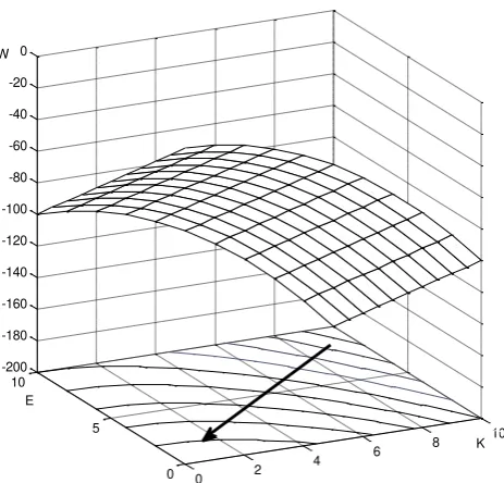
Consequently, the economic energy efficiency function is
= 2 1
This function can be visualized in Figure 4. We can see that the projection of W surface
lies in the E—K plane and the energy efficiency increases following the direction of the
arrow. Indeed, the curves in E—K plane are the ones have been illustrated in Figure 2.
Every curve represents a state of efficiency. The process of increasing energy efficiency
[image:16.595.214.446.488.710.2]is the process of climbing the curves.
Figure 4 The simulation of economic energy efficiency function
Next, I will simulate the optimal paths of K and E. Note that usually, the capital stock 0 2
4 6
8 10 0
5 10
-200 -180 -160 -140 -120 -100 -80 -60 -40 -20 0 W
E
K>>0. Given the numerical example, A ≈ . Hence, the function of K is
= ( . .1 .1𝑡 .1𝑡 . ) .
.7
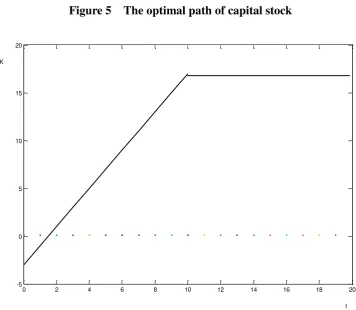
[image:17.595.145.502.195.505.2]The curve is drawn in Figure 5.
Figure 5 The optimal path of capital stock
As Figure 5 illustrated, the path of capital stock increases at first, after ten periods, it
will remain constant.
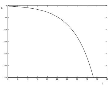
On the side of energy consumption, the simulated function is
= .1𝑡 1.
The path can be investigated in Figure 6. As we can see, the energy consumption will
always decline over time. Besides, its speed is slow at first but becomes more and more
rapidly then.
0 2 4 6 8 10 12 14 16 18 20 -5
0 5 10 15 20
K
Figure 6 The optimal path of energy consumption
5
Discussion
The modelling and results reveal some interesting policy implications.
Firstly, under the neoclassical growth mechanism and investment constraint, we can get
the maximum of economic energy efficiency continuously. Even though the economic
energy efficiency has two meanings including reducing the energy distance and
climbing the best efficient curves, the optimization modelling mainly reflects the latter
one and focus on long-term effect. In this paper, technology progress is assumed
exogenous and it is an underlying reason for energy efficiency improvement in long-run.
In other words, the effect of technology is not direct but embodied by investment in this
model. For achieving the maximum efficiency, the economy should run in the optimal
investment state by energy consumption being controlled. In reality, energy
consumption is relative easy to control for many developing countries as investment is a
fluctuant variable in many circumstances.
0 5 10 15 20 25 30 35 40 45 50 -300
-250 -200 -150 -100 -50 0
E
The second important thing is about the state of equilibrium. The saddle-point reveals
that there is the only stable branch to reach the target point Q. If the economy gets onto
the unstable branch unfortunately, it could never reach the optimization. Thus, the path
choice is still vital for social planners. Additionally, the phrase—diagram indicates that
the increase in investment is accompanying with an increase in the rate of energy
consumption. This is proved by Figure 5 and 6 in the numerical simulation.
Next, we discuss the two transition paths of state variable and control variable. The
result in Figure 5 is in accord with the statement of Solow model. After the steady state,
the capital stock will not increase. In other words, the investment is only equal to the
depreciation of capital. Hence, even though energy consumption is included in Solow
model, it does not change the basic conclusion of neoclassical growth model. On the
other hand, the curve in Figure 6 is also easy to understand. With the continuous
improvement of energy efficiency, the amount of energy consumption is decreasing all
the time. Initially, the rate of decline is small. But with the accumulation of technology
and capital, the rate of decline becomes more faster. As capital will not change over ten
periods, technology will be a key factor in long-run. Thus, the shift of slope can be
explained by the scale effect of technology.
Lastly, the imposed restriction that the population is constant is somewhat unreasonable.
It is mainly for getting an appropriate solution in modelling. In fact, population is
always increasing in many developing countries. However, this restriction could also
remind governments in those countries that population plan could be important for a
better development.
6
Conclusion
The modelling on the dynamic optimization demonstrates some implications and
inspirations. In development, energy efficiency is a key factor linking with other
macroeconomic variables. On one hand, industrialization and modernization lead to the
appetite for energy. The improvement of energy efficiency is essential for utilizing and
largely depends upon the investment and technology, which are key drivers in
development. Pursuing the maximum energy efficiency is not contradictory with
investing and consuming energy. In contrast, they can be harmonized in growth and
development. This fact could help developing countries crucial for developing countries
realize a sustainable development.
Moreover, the modelling provides specific methods for approaching a better
development. As the extended Solow model works well, governments can energy
consumption effectively and make the optimal state of investment at any time. As a
result, the levels of best energy efficiency could be attained in succession; the capital
stock will increase until reaching the steady level of the golden rule which is illustrated
in Solow model; while the energy consumption will decline continuously. Eventually,
References
Brennan, TJ 2010, 'Optimal energy efficiency policies and regulatory demand-side
management tests: How well do they match?', Energy Policy, Vol. 38, pp. 3874-3885.
Chiang, AC 1992, 'Chapter 7: optimal control', in Elements of Dynamic Optimization,
Waveland Press, Illinois, pp. 200-204.
Conrad, K 2001, 'The optimal path of energy and CO2 taxes for intertemporal resource
allocation', CESifo Working paper, no.552, viewed 20 November 2012,
<http://www.cesifo-group.de/portal/pls/portal/docs/1/1190566.PDF>
Dasgupta, PS & Heal, GM 1979, Economic theory and exhaustible resources, Oxford
University Press, UK.
Forster, BA 1980, 'Optimal energy use in a polluted environment', Journal of
Environmental Economics and Management, Vol.7, pp. 321-333.
Garg, PC & Sweeney, JL 1978, 'Optimal growth with depletable resources', Resources
and Energy, Vol. 1, pp. 43-56.
Jaffe, AB & Stavins, RN 1994, 'The energy-efficiency gap', Energy Policy, vol.22, no.10,
pp. 804-810.
Jin, Y & Arons, JS 2009, 'Chapter 3: the metabolic society', in Resource, Energy,
Environment, Society: Scientific and Engineering Principles for Circular Economy,
Chemical Industry Press, Beijing, pp. 92-93.
Li, H, Long, R & Lan, X 2012, 'Economic growth in resource-based cities: based on
ecological constrains', China Soft Scinece Magazine, vol.26, no.6, pp. 53-59.
Lucas, R 1988, 'On the mechanics of economic development', Journal of Monetary
National Bureau of Statistics of China, 2010, Handbook of Energy Statistics, China
Statistics Press, Beijing.
Peng, S 2007, 'Natural resource depletion and sustainable economic growth based on a
four-sector endogenous growth model', Journal of Industrial Engineering and
Engineering Management, vol.21, no.4, pp. 119-124.
Perrot, P 1998, A to Z of Thermodynamics, Oxford University Press, England.
Pindyck, RS 1978, 'The optimal exploration and production of nonrenewable resources',
Journal of Political Economy, vol.86, no.5, pp. 841-861.
Pindyck, RS 1980, 'Uncertainty and exhaustible resource markets', Journal of Political
Economy, vol.88, no.6, pp. 1203-1225.
Romer, PM 1990, 'Endogenous technological change', Journal of Political Economy,
Vol.98, pp. 71-102.
Sanchez, JA & Ruiz, PM 2009, 'Locally optimal source routing for energy-effiency
geographic routing', Wireless Netw, Vol.15, pp. 513-523.
Stern, DI 2011, 'The role of energy in economic growth', Annals of the New York
Academy of Sciences, pp. 26-51.
Stern, DI 2012, 'Modelling international trends in energy efficiency', Energy Economics,
Vol. 34, pp. 2200-2208.
Stiglitz, J 1974, 'Growth with exhaustible natural resources: efficient and optimal
growth paths', Review of Economic Studies, Vol.41, pp. 123-137.