Hydrologic extremes – an intercomparison of multiple gridded statistical downscaling methods

www.hydrol-earth-syst-sci.net/20/1483/2016/ doi:10.5194/hess-20-1483-2016

© Author(s) 2016. CC Attribution 3.0 License.

Hydrologic extremes – an intercomparison of multiple gridded

statistical downscaling methods

Arelia T. Werner1and Alex J. Cannon2

1_{Pacific Climate Impacts Consortium, Victoria, British Columbia, Canada}

2_{Climate Research Division, Environment and Climate Change Canada, Victoria, British Columbia, Canada}

Correspondence to: Arelia T. Werner ([email protected])

Received: 22 April 2015 – Published in Hydrol. Earth Syst. Sci. Discuss.: 26 June 2015 Revised: 4 March 2016 – Accepted: 17 March 2016 – Published: 19 April 2016

Abstract. Gridded statistical downscaling methods are the main means of preparing climate model data to drive dis-tributed hydrological models. Past work on the validation of climate downscaling methods has focused on tempera-ture and precipitation, with less attention paid to the ulti-mate outputs from hydrological models. Also, as attention shifts towards projections of extreme events, downscaling comparisons now commonly assess methods in terms of cli-mate extremes, but hydrologic extremes are less well ex-plored. Here, we test the ability of gridded downscaling models to replicate historical properties of climate and hy-drologic extremes, as measured in terms of temporal se-quencing (i.e. correlation tests) and distributional proper-ties (i.e. tests for equality of probability distributions). Out-puts from seven downscaling methods – bias correction constructed analogues (BCCA), double BCCA (DBCCA), BCCA with quantile mapping reordering (BCCAQ), bias correction spatial disaggregation (BCSD), BCSD using min-imum/maximum temperature (BCSDX), the climate imprint delta method (CI), and bias corrected CI (BCCI) – are used to drive the Variable Infiltration Capacity (VIC) model over the snow-dominated Peace River basin, British Columbia. Out-puts are tested using split-sample validation on 26 climate extremes indices (ClimDEX) and two hydrologic extremes indices (3-day peak flow and 7-day peak flow). To charac-terize observational uncertainty, four atmospheric reanaly-ses are used as climate model surrogates and two gridded observational data sets are used as downscaling target data. The skill of the downscaling methods generally depended on reanalysis and gridded observational data set. However, CI failed to reproduce the distribution and BCSD and BCSDX the timing of winter 7-day low-flow events, regardless of

re-analysis or observational data set. Overall, DBCCA passed the greatest number of tests for the ClimDEX indices, while BCCAQ, which is designed to more accurately resolve event-scale spatial gradients, passed the greatest number of tests for hydrologic extremes. Non-stationarity in the observa-tional/reanalysis data sets complicated the evaluation of downscaling performance. Comparing temporal homogene-ity and trends in climate indices and hydrological model out-puts calculated from downscaled reanalyses and gridded ob-servations was useful for diagnosing the reliability of the var-ious historical data sets. We recommend that such analyses be conducted before such data are used to construct future hydro-climatic change scenarios.

1 Introduction

Ouarda, 2009). Conversely, Canadian annual low-flow in-dices showed spatially uniform decreases over 1970 to 2005 (Monk et al., 2011). Thus, future changes in hydrologic ex-tremes need to be estimated at regionally relevant resolutions (∼10 km) and consider both temperature and precipitation effects.

Global climate models (GCMs) are one of our only tools for projecting the future climate, but they operate at scales too coarse (∼100 km) for use in regional studies. Hence, be-fore projecting changes in hydrologic extremes, some inter-vening steps are required. Approaches to converting coarse-scale GCM simulations to project changes to peak flows and low flows vary. Some examples include direct down-scaling of streamflow extremes by sparse Bayesian learning and multiple linear regression (Joshi et al., 2013), weather generators combined with hydrologic models (Cunderlik and Simonovic, 2007), regional frequency analysis of re-gional climate model (RCM) projections (Clavet-Gaumont et al., 2013), and, most commonly, statistical downscaling of GCM or RCM projections run through a physically based hydrologic model (Elsner et al., 2010a; Maurer et al., 2010; Schnorbus et al., 2014; Shrestha et al., 2012; Bürger et al., 2011). The uncertainty in hydrologic projections from GCMs is greater than that from emissions scenarios or model parameterizations (Bennett et al., 2012; Prudhomme and Davies, 2008) and all GCMs represent the climate imper-fectly in different ways (Gleckler et al., 2008; Knutti et al., 2008); therefore, to fully characterize the uncertainty in projected hydrological extremes, an ensemble of GCMs is required.

Gridded statistical downscaling methods provide a com-putationally efficient and effective means of producing plau-sible hydro-climatology from a large ensemble of GCMs (Salathe et al., 2007; Salathé, 2005; Wood et al., 2004). A number of studies have compared multiple statistical down-scaling methods for use in climatological or hydrologi-cal projections. Maurer and Hidalgo (2008) compared con-structed analogues (CA) and bias correction spatial disag-gregation (BCSD) using the National Centers for Environ-mental Prediction/National Center for Atmospheric Research Reanalysis I (NCEP1) (Kalnay et al., 1996) as a surrogate GCM. Methods were comparable in producing precipitation and temperature at a monthly and seasonal level, but skil-fully downscaled daily data depended on the ability of the climate model to show daily skill. Bürger et al. (2012a) com-pared five methods for their ability to represent climatic ex-tremes including BCSD and expanded downscaling (XDS). The fixed diurnal temperature range in BCSD was seen as a shortcoming in Bürger et al. (2012a). XDS performed best, passing 48 % of single tests on average for 27 Climate In-dices of Extremes (ClimDEX), with BCSD close behind, passing 45 % (Bürger et al., 2012a). Pierce et al. (2013) found that projected increases in annual precipitation versus de-creases in California were due to disagreements in the oc-currence of the heaviest precipitation days (>60 mm day−1)

amongst three dynamical and two statistical downscaling methods (BCCA and BCSD). Maurer et al. (2010) compared BCSD, BCCA, and CA for their ability to reproduce hydro-logic extremes. BCCA, when combined with the Variable In-filtration Capacity (VIC) model, consistently outperformed the other methods in simulating 3-day peak flow and 7-day low flow. BCCA is an improvement over CA because it in-cludes bias correction and over BCSD because it inin-cludes daily GCM anomalies (Maurer et al., 2010). An additional method described as statistical downscaling and bias cor-rection (Abatzoglou and Brown, 2012) and as asynchronous regression (Gutmann et al., 2014), both of which interpo-late from the GCM to a fine scale and then apply quantile mapping bias correction (i.e. basically reversing the steps of BCSD), was found to reproduce extreme precipitation events at the grid scale but overestimate them on aggregate scales (Maraun, 2013). Studies to date have not assessed the strength of downscaling methods for use with climatic and hydrologic extremes concurrently.

Gridded climate observations underpin hydrologic pro-jections. They are used to calibrate the downscaling tech-nique and the hydrologic model, serving as targets and in-puts, respectively. Gridded observations are commonly eval-uated via comparison with station observations (Hutchinson et al., 2009; Werner et al., 2015), intercomparison with other gridded observations (Eum et al., 2014), or by using them to drive a hydrologic model and comparing outputs to ob-served water balance fluxes and streamflow over large basins (Livneh et al., 2013; Maurer et al., 2002). We know that statistical downscaling methods perform poorly when non-stationarity occurs between the calibration and validation pe-riods (Maurer et al., 2013), but we have not evaluated how apparent non-stationarity caused by natural climate variabil-ity (Huang et al., 2014; Maraun, 2012) is amplified or di-minished with methods used to create gridded observations, which could also affect the success of downscaling methods. Furthermore, stationarity in mean annual precipitation and temperature does not dictate stationarity in climatic or hy-drologic extremes. Not all, but some, previous studies have included as many years as possible in the calibration, with the goal of maximizing the available historical record available for resampling in the temporal disaggregation step applied in BCSD (Bürger et al., 2012a; Salathé, 2005; Werner, 2011). This approach is also supported by other studies that found bias correction is more robust for larger samples from longer time series, especially for extremes such as flood events (Huang et al., 2014; Themeßl et al., 2011). The pros and cons of this extended calibration period have not been fully eval-uated. This investigation will help the hydrologic modelling community build a better evaluation system for gridded ob-servations to ensure their strength not only for projections of mean monthly changes over large basins∼100 000 km2, but also for extremes in basins as small as 500 km2.

When used to make climate change projections, dis-tributed hydrologic models such as VIC are best driven with gridded daily data, which is usually produced via gridded statistical downscaling techniques such as BCSD, CA, and BCCA, three gridded methods that have been tested to date. Applying BCSD using minimum and maximum monthly temperature instead of mean monthly temperature has not been tested and may correct some issues with diurnal tem-perature range (Bürger et al., 2012a). It is important to note that the effect of BCSD on daily temperature range (DTR) when used with daily data and ways to ensure minimum temperature is less than maximum temperature has been tested by Thrasher et al. (2012) and is not the focus of this study. A few other methods have been developed recently that warrant investigation. These include double bias cor-rected constructed analogue (DBCCA), which is similar to BCCA but applies a second quantile mapping bias correc-tion as a post-processing step to correct drizzle and other residual biases (Maurer et al., 2010). Additionally, the cli-mate imprint delta method (CI) (Hunter and Meentemeyer, 2005) and the “reverse” BCSD (similar to SDBC in Ahmed

et al., 2013, and AR in Gutmann et al., 2014), which we refer to as bias corrected climate imprint (BCCI) due to its use of CI for interpolation, have not been explored for their applicability to hydrology. A recently developed hy-brid of BCCA and BCCI, referred to as BCCAQ (Cannon et al., 2015; Murdock et al., 2014), has the potential to be an improvement versus other gridded statistical downscaling techniques and has not been tested with hydrologic extremes. This work will also help to inform use of the resulting BCSD and hydrologic model output provided by the Pacific Cli-mate Impacts Consortium (PCIC; http://www.pacificcliCli-mate. org/data). Finally, PCIC also makes available Canada-wide downscaled climate change projections using both the BCSD and BCCAQ methods (http://www.pacificclimate.org/data). This study provides the first rigorous intercomparison of these two methods.

The ClimDEX indices are recommended by the World Meteorological Organization Expert Team on Climate Change Detection and Indices (ETCCDI) (Zhang et al., 2011) as a means of summarizing daily temperature and precipitation statistics, focusing particularly on aspects of climate extremes. They have been developed to allow seam-less comparison of climate conditions on an international basis. There are many projects applying the ETCCDI in-dices to detect changes in extremes historically (e.g. mann et al., 2013a), to project future changes (e.g. Sill-mann et al., 2013b), and to provide future changes via data portals to allow local analysis (http://www.cccma.ec.gc.ca/ data/climdex/). Two commonly investigated hydrologic ex-tremes include 3-day peak flow, which represents potential flood conditions, and 7-day low flow, which represents po-tential drought conditions (e.g. Maurer et al., 2010). Floods can be damaging to river and floodplain infrastructure, while droughts can be detrimental for human water use and aquatic habitat. We follow the framework developed by Bürger et al. (2012a), evaluating methods for their abilities in produc-ing the temporal sequencproduc-ing and distributional properties of climate indices and hydrologic extremes.

The objectives of this study are the following.

1. To compare several reanalyses in the study region against two gridded observation data sets.

2. To test the ability of the BCCA, DBCCA, BCCI, CI, BCSD (mean temperature), BCSDX (minimum and maximum temperature), and BCCAQ downscaling techniques to simulate 26 ClimDEX indices using four reanalyses and two gridded observations.

4. To learn more about the strengths and weaknesses of two gridded observations for use with hydrologic mod-elling.

5. To see whether the strength of a method to downscale for climate extremes relates to abilities for use with hy-drologic extremes.

2 Study area

The Peace River basin will be the focus of this work. The snow-dominated regime of this basin makes the findings of this work applicable to many mid-latitude areas. The Peace River is located in interior north-eastern BC and encom-passes the 101 000 km2drainage area upstream of Taylor, BC (Fig. 1). Elevations range from 400 to 2800 m. The region is highly influenced by the Pacific Ocean and Arctic air masses. The region has a continental climate (Demarchi, 1996), with monthly average temperatures ranging from−12.0◦C in Jan-uary to 12.3◦C in July, averaging 0.2◦C. Precipitation fol-lows a seasonal pattern of summer maximum and spring min-imum. The Peace River has a nival regime, with approxi-mately 54 % of the annual precipitation (440 mm) falling as snow (mostly during October–April) and 64 % of the natural streamflow occurring during the freshet months of May–July. Low flows occur during the winter and early spring in head-water (INGEN) and downstream (BCGMS) basins (Fig. 2). Due to the topographical complexity and strong climate gra-dients this region provides a stringent test of downscaling techniques. Additionally, the Peace River basin is the focus of two studies that explore uncertainty in hydrologic projec-tions, one due to GCMs, emissions scenarios, and parameter sets (Bennett et al., 2012), the other due to statistically ver-sus dynamically downscaled GCMs (Shrestha et al., 2014a). This study provides a good complement to these by exploring new sources of uncertainty in the same basin.

3 Methods

3.1 Gridded observations

Two daily, gridded observational data sets were available over the study area. The first was generated for BC for appli-cation with the Variable Infiltration Capacity (VIC) macro-scale distributed hydrologic model following the methods of Maurer et al. (2002) and Hamlet and Lettenmaier (2005). Daily gridded surfaces of minimum and maximum temper-ature and daily precipitation accumulation were produced at the spatial resolution of 1/16◦, which is ∼6 km2 depend-ing on latitude, for January 1950 to December 2005. Sta-tion data were contributed from multiple networks includ-ing those of Environment Canada, BC Ministry of Forests, Lands and Natural Resource Operations, BC Hydro, and the US National Weather Service Co-operative Observer

Pro-Figure 1. The Peace River basin (above Taylor, BC) study area

analysed for ClimDEX indices (black boundary) and the five sub-basins investigated for hydrologic extremes, including the Finlay River above the Akie River (FINAK), the Ingenika River above the Swannell River (INGEN), the Parsnip River above the Misinchinka River (PARMS), the Peace River above the Pine River (PEAPN), and the Peace River at Bennett Dam (BCGMS).

−100 0 100 200

0

2000

4000

6000

8000

Discharge

(

m

3 se

c

−

1 )

OCT NOV DEC JAN FEB MAR APR MAY JUN JUL AUG SEP

Day of year

BCGMS 5th−25th % / 75th−95th %

25th−75th % Median

−100 0 100 200

0

100

200

300

400

500

600

Discharge

(

m

3se

c

−

1)

OCT NOV DEC JAN FEB MAR APR MAY JUN JUL AUG SEP

Day of year

INGEN 5th−25th % / 75th−95th %

25th−75th % Median

Figure 2. Annual daily hydrograph 1985–1995 for the (top)

gram, each with a varying range of quality control. Stations were interpolated to grids using the SYMAP inverse-distance weighting algorithm (Shepard et al., 1984). The raw grid-ded fields were temporally homogenized to remove inter-polation artefacts introduced by using a temporally varying mix of stations and corrected for topographic effects using ClimateWNA, a 1961–1990 PRISM based high-resolution climatology for western North America (Daly et al., 1994; Wang et al., 2006). This data set is referred to as VIC Forc-ings.

The second data set was created for all of Canada using the Australian National University Spline (ANUSPLIN) imple-mentation of trivariate thin plate smoothing splines (Hutchin-son et al., 2009). The Canada-wide ANUSPLIN observa-tional data set was created at a 1/12◦grid spacing (∼10 km) for daily minimum temperature, maximum temperature, and precipitation amounts for the period 1950–2010 by Hopkin-son et al. (2011) and McKenney et al. (2011). Station data from Environment Canada observing sites were interpolated onto the high-resolution grid using the ANUSPLIN smooth-ing splines with elevation, longitude, and latitude as inter-polation predictors. Precipitation occurrence and square-root transformed precipitation amounts were interpolated sepa-rately on each day, combined, and transformed back to orig-inal units. Observed station data were quality controlled and corrected for station relocation, changes in the definition of the climate day, and trace precipitation amounts.

3.2 Reanalyses

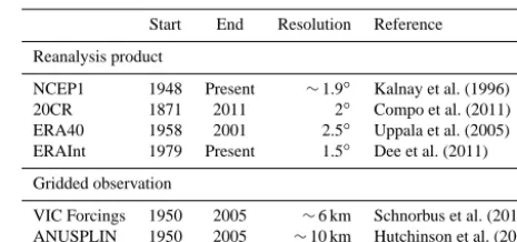
Four atmospheric reanalysis products were selected to span a range of complexity and spatial resolution. Chosen meth-ods include NCEP1, European Centre for Medium-Range Weather Forecasts (ECMWF) Re-Analysis 40 (ERA40), ECMWF Re-Analysis Interim (ERAInt), and the National Oceanic and Atmospheric Administration – Cooperative In-stitute for Research in Environmental Sciences 20th Century Reanalysis V2 (20CR). NCEP1 is a popular reanalysis prod-uct applied in the validation of statistical downscaling tech-niques (Bürger et al., 2012a; Maurer et al., 2010). It spans the period from 1948 to the present, is∼1.9◦in resolution, and includes a wide range of observations assimilated from ship to satellite data (Kalnay et al., 1996). ERA40 is available from 1958 to 2002 and is archived at the coarsest resolution (2.5◦) of the four products selected for this study. It was the first to assimilate satellite radiance data directly (Uppala et al., 2005). ERAInt covers the satellite era from 1979 through to the present. Data used here are archived at 1.5◦_{, although}

the underlying forecast model runs at 0.75◦. It has an im-proved atmospheric model and assimilation system over that used in ERA40 (Dee et al., 2011). 20CR is one of the longest reanalysis records available, starting in 1871 and running to 2012. At 2◦ resolution it assimilates only surface observa-tions of synoptic pressure, monthly sea surface temperature and sea ice distribution (Compo et al., 2011). Table 1

sum-Table 1. Availability of gridded observations and reanalyses.

Start End Resolution Reference

Reanalysis product

NCEP1 1948 Present ∼1.9◦ _{Kalnay et al. (1996)}

20CR 1871 2011 2◦ Compo et al. (2011) ERA40 1958 2001 2.5◦ Uppala et al. (2005) ERAInt 1979 Present 1.5◦ Dee et al. (2011)

Gridded observation

VIC Forcings 1950 2005 ∼6 km Schnorbus et al. (2014) ANUSPLIN 1950 2005 ∼10 km Hutchinson et al. (2009)

marizes the availability of the gridded observations and re-analyses.

3.3 Downscaling techniques

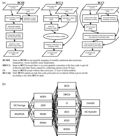
Seven statistical approaches are selected based on their wide use and/or potential strength in downscaling coarse-scale models to gridded observations for representing extremes. BCSD has been applied across North America (Maurer and Hidalgo, 2008; Salathé, 2005; Schnorbus et al., 2014; Wood et al., 2002, 2004). Monthly minimum temperature, maxi-mum temperature, and precipitation from GCMs or reanaly-ses are bias corrected, using quantile mapping, against grid-ded observations aggregated to the large-scale model grid. Bias corrected, spatially disaggregated monthly data are tem-porally disaggregated to a daily time step via random sam-pling of historical months. Days in the selected month are rescaled (multiplicative for precipitation and additive for temperature) to match the bias corrected monthly precipi-tation and average temperature (Fig. 3a). Two variations of BCSD are tested; one derives minimum and maximum tem-perature from mean temtem-perature in the coarse-scale model by assuming a uniform monthly diurnal temperature range (BCSD); the other uses monthly minimum and maximum temperature directly from the large-scale model (BCSDX).

Figure 3. (a) Diagram of the bias corrected spatial disaggregation (BCSD), bias corrected constructed analogues (BCCA), and bias corrected

climate imprint (BCCI) downscaling methods and a summary of adjustments made to these methods to create BCSD with monthly minimum and maximum temperature (BCSDX), double BCCA (DBCCA), climate imprint (CI), and BCCA corrected to BCCI (BCCAQ). (b) Workflow diagram for assessment of downscaling techniques in replicating ClimDEX and hydrologic extremes.

Two climate imprint methods are tested, the CI delta method (Hunter and Meentemeyer, 2005) and bias corrected CI (BCCI), which applies quantile mapping to the interpo-lated series from CI (Fig. 3a). For the imprint methods, long-term averages (i.e. 30 years) from the fine-scale data pro-vide a “spatial imprint” that is used to represent environmen-tal gradients. The ratio of daily to average monthly values is multiplied by the fine-scale monthly values for a location to get the daily precipitation. This is similar for minimum and maximum temperature, except values are calculated as

the difference between the monthly mean and the daily value (Hunter and Meentemeyer, 2005).

Be-cause the optimal weights used to combine the analogues in BCCA are derived on a day-by-day basis, without reference to the full historical data set, the algorithm may be prone to Huth’s paradox, wherein models that are calibrated based on short-term variability may be biased and fail to produce re-alistic long-term trends (Benestad et al., 2008; Huth, 2004). Reordering data for each fine-scale grid point within a month effectively breaks the overly smooth representation of sub reanalysis-grid-scale spatial variability inherited from BCCI (Maraun, 2013), thereby resulting in a more accurate repre-sentation of event-scale spatial gradients; this also prevents the downscaled outputs from drifting too far from the BCCI long-term trend. Over longer timescales, the spatial variabil-ity of BCCAQ converges to that of BCCI.

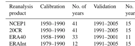
Statistical methods are calibrated from 1950 to 1990 for 20CR and NCEP1, and from 1958 to 1990 and from 1979 to 1990 for ERA40 and ERAInt, respectively (Table 2). Cal-ibration periods were selected to include the longest over-lapping record between the gridded observation and reanal-yses to replicate the approach taken in Werner et al. (2011). Thus, the 20CR and NCEP1 reanalyses results will serve to evaluate the gridded observations and these two reanalyses, and also to validate the calibration–validation approach taken with BCSD for a series of studies conducted in this region (Bürger et al., 2012a, b; Schnorbus et al., 2014; Shrestha et al., 2012; Werner et al., 2013). The resulting modelling framework for these two gridded observations, four reanaly-sis products, and seven gridded statistical downscaling tech-niques is displayed in Fig. 3b. All statistical downscaling methods use precipitation and temperature as predictors and predictands.

3.4 ClimDEX

ClimDEX is a common climate indices package that com-putes values for 27 core indices based on daily precipi-tation and minimum and maximum temperature (Karl et al., 1999; Peterson, 2005; and http://etccdi.pacificclimate.org or http://www.clivar.org/panels-and-working-groups/etccdi/ etccdi.php/). These indices describe events such as the num-ber of heavy precipitation days denoted as days where pre-cipitation is greater than 10 mm or percentage of days when maximum temperature is greater than the 90th percentile. They do not usually represent the most extreme events con-ceivable, but instead represent “the more extreme aspects of climate”, which are known to be relevant to a broad range of impact fields and are still statistically manageable, so that they can be reliably estimated from current data for the present and future. ClimDEX has been adopted as a standard for extremes by the World Climate Research Programme (http://www.clivar.org/organization/extremes). Indices were computed from downscaled temperature and precipitation from seven statistical downscaling methods used with four reanalyses and two gridded observations for a total of 56 estimates of each index. The index of the annual count

Table 2. Calibration and validation periods for downscaling

meth-ods by reanalyses.

Reanalysis Calibration No. of Validation No. of

product years years

NCEP1 1950–1990 41 1991–2005 15

20CR 1950–1990 41 1991–2005 15

ERA40 1958–1990 33 1991–2001 11

ERAInt 1979–1990 12 1991–2005 15

when daily minimum temperature is>20◦C, tropical nights (tr), was dropped for this analysis because this temperature threshold is not exceeded in the Peace River basin. See Ta-ble 1 in Bürger et al. (2012a) for a description of indices ex-plored in this study.

3.5 Hydrologic modelling

Hydrologic projections for the Peace River basin are de-rived using the Variable Infiltration Capacity (VIC) model (Liang et al., 1994, 1996). The VIC model is a spatially dis-tributed macro-scale hydrologic model that was originally developed as a soil–vegetation atmosphere transfer scheme for general circulation models. It has been used to evalu-ate climevalu-ate change impacts on global river systems (Nijssen et al., 2001) and in the mountainous western United States and BC (Elsner et al., 2010b; Hamlet and Lettenmaier, 2005, 2007; Schnorbus et al., 2014; Shrestha et al., 2012). Its spa-tially distributed nature makes it suitable for capturing re-gional variation in the hydrologic cycle due to topographic, physiographic, and climatic controls. The VIC model is also process based, allowing for a more plausible extrapolation of hydrologic processes into future climate regimes (Leavesley, 1994). The VIC model is applied at a resolution of 1/16◦ (ap-proximately 27–31 km2, depending upon latitude) and run at a daily time step (1 h time step for the snow model). Surface routing between grid cells is done using the linearized Saint-Venant equations (Lohmann et al., 1996).

er-Table 3. Metadata for five select sub-basins of the Peace River basin.

Basin Water Survey of Canada Drainage area Elevation

ID (km2) (m)

Mean Min Max

BCGMS – 72 078

FINAK 07EA005 16 000 1452 693 2799

INGEN 07EA004 4200 1503 674 2289

PARMS 07EE007 4900 1128 645 2343

PEAPN 07FA004 83 900 1126 392 2799

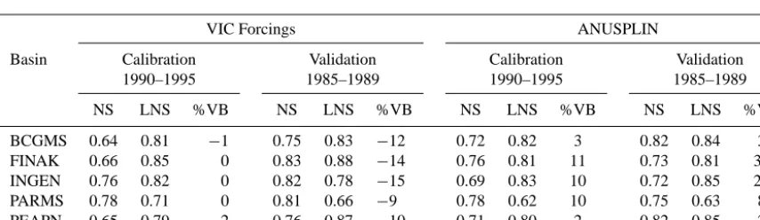
Table 4. Calibration and validation statistics for five select sub-basins of the Peace River basin under the under VIC Forcings and ANUSPLIN

gridded observational data sets including the Nash–Sutcliff efficiency score (NS), the Nash–Sutcliff efficiency score of the log-transformed discharge (LNS), and the percent volume bias error (%VB).

VIC Forcings ANUSPLIN

Basin Calibration Validation Calibration Validation

1990–1995 1985–1989 1990–1995 1985–1989

NS LNS %VB NS LNS %VB NS LNS %VB NS LNS %VB

BCGMS 0.64 0.81 −1 0.75 0.83 −12 0.72 0.82 3 0.82 0.84 3

FINAK 0.66 0.85 0 0.83 0.88 −14 0.76 0.81 11 0.73 0.81 30

INGEN 0.76 0.82 0 0.82 0.78 −15 0.69 0.83 10 0.72 0.85 26

PARMS 0.78 0.71 0 0.81 0.66 −9 0.78 0.62 10 0.75 0.63 8

PEAPN 0.65 0.79 −2 0.76 0.87 −10 0.71 0.80 2 0.82 0.85 2

ror differences became larger in magnitude in the 1985–1989 split-sample validation period, negative in VIC Forcings, and positive in ANUSPLIN.

There are several daily streamflow metrics that are useful for water resources design and management, which are also ecologically relevant (Monk et al., 2011; Richter et al., 1996; Shrestha et al., 2014b). A recent intercomparison of statis-tical downscaling techniques for use with daily streamflow investigated the hydrologic extremes 3-day peak flow and 7-day low flow (Maurer et al., 2010). To build on that study we investigate the strength of seven downscaling methods for the same metrics using 3-day peak flow to represent flood and, 7-day low flow, drought. Two low-flow periods are investi-gated because the lowest discharge takes place in the months of October–April in sub-basins of the Peace River (Fig. 2) and summer low flows (July–September) are of interest to agriculture and ecology. Hydrologic models can have low flows in different seasons than observations due to their poor parameterization of baseflow conditions and because calibra-tion approaches favour good performance for peak flow (Na-jafi et al., 2011). This issue can be exaggerated by down-scaling approaches (Shrestha et al., 2014b). Thus, narrowing the window over which low flows are accessed is important to prevent low flows in one season being compared to low flows in another. Peak flows are analysed between May and July.

3.6 Statistical tests

The seven statistical downscaling methods vary in their ap-proach, which can result in differing strengths and weak-nesses. We chose our statistical tests to fully evaluate these downscaling techniques for the climate and hydrologic re-sults and to follow the framework of Bürger et al. (2012a). The time period for calibration of the downscaling tech-niques was selected to match Bürger et al. (2012a) (pre-1991, depending on the availability of the reanalyses). Longer cal-ibration periods available for NCEP1 and 20CR were also seen as favourable when applying bias correction based downscaling methods, especially when working with ex-tremes (Huang et al., 2014; Themeßl et al., 2011), and as-sisted with evaluating the two gridded observations. Vali-dation was set to 1991–2005 to accommodate the overlap of available reanalyses, gridded observations, and observed streamflow records. ERA40 is an exception, with the last full year of available record for 2001. Validation results for ERA40 are provided for 1991–2001.

hypoth-esis is expected to occur (so-called type I error) and the rate at which a given test will correctly reject the null hypothe-sis when it is false (the so-called power of the test), with the choice of a more conservative significance level, such as 1 %, leading to lower power in exchange for a lower type-I error rate (e.g. von Storch and Zwiers, 1999).

Two statistical tests are applied to the ClimDEX results over the Peace River basin: the Kolmogorov–Smirnov (KS) test and the test for Pearson’s correlation. The KS test is used to see how well the distribution of climate indices for the statistically downscaled reanalyses matches the distribution of those calculated from the gridded observations used as downscaling targets. The KS test is a nonparametric test of the equality of continuous one-dimensional probability dis-tributions. Here, it is used to compare two samples, namely annual climate indices for the statistically downscaled re-analyses and the associated gridded observation. The KS test statistic is used to quantify the distance between empirical distribution functions of these two samples. The null hy-pothesis is that the two samples are drawn from the same distribution. The distributions considered under the null hy-pothesis have to be continuous distributions, but are other-wise unrestricted. While some of the climate indices are not strictly continuous (e.g. frost days), asymptotic critical val-ues may still be used in the presence of a small number of ties (Janssen, 1994). Pearson’s correlation is used to test the temporal correspondence between the annual climate indices for the statistically downscaled reanalyses and the associated gridded observation. Pearson’s product moment correlation coefficient is used to measure the linear correlation between climate indices from downscaled reanalyses and indices from observations. The null hypothesis is that the downscaled and observed samples are not linearly correlated.

The 101 000 km2Peace River basin is represented by 3975 grid cells at the 1/16◦resolution used to run the VIC hydro-logic model. The KS test and Pearson’s correlation are eval-uated on each of the grid cells in the Peace River basin for each climate index. The statistical significance of the KS test and Pearson’s correlation results over the basin as a whole are measured using a field significance test: the Walker field significance test (Wilks, 2006), where the evaluation of field significance is done by using the minimum localpvalue as the global test statistic. The Walker field significance test was selected because it is relatively insensitive to correla-tions among local tests, allowing global tests based on data exhibiting both spatial and temporal correlations to be con-ducted. Temporal and spatial correlations between climate indices grids would require a cumbersome procedure to ad-dress correctly with conventional resampling tests. Walker’s test can be seen to be closely related to the conventional field significance test (Storch, 1982) based on counting significant local results, except that Walker’s test statistic is based on the smallest of theK localpvalues, rather than the number of

Klocal tests that are significant at some level.

The KS test and the test for Pearson’s correlation were ap-plied to the 3-day peak flow and 7-day low flow in winter and summer for hydrologic data from the five sub-basins of the Peace River. In this case, with the KS test the null hypothe-sis is that the distribution of the hydrologic extremes created by driving the VIC model with the statistically downscaled reanalyses are drawn from the same sample as those derived from driving the VIC model with the two gridded observa-tions. The null hypothesis for Pearson’s correlation is that the hydrologic extremes created by driving VIC with down-scaled reanalyses versus gridded observations are not linearly correlated.

4 Results

4.1 Gridded observations and reanalyses

1950 1960 1970 1980 1990 2000

−40

−30

−20

−10

Jan

1950 1960 1970 1980 1990 2000

−25

−20

−15

−10

−5 Feb

1950 1960 1970 1980 1990 2000

−20

−15

−10

−5

Mar

1950 1960 1970 1980 1990 2000

−15

−10

−5

0 Apr

1950 1960 1970 1980 1990 2000

−5

0

5

May

1950 1960 1970 1980 1990 2000

05

1

0 Jun

1950 1960 1970 1980 1990 2000

0

5

10

15

Jul

1950 1960 1970 1980 1990 2000

2468

1

0

1

2 Aug

1950 1960 1970 1980 1990 2000

−

4

02468

1

0

Sep

1950 1960 1970 1980 1990 2000

−10

−5

0

5 Oct

1950 1960 1970 1980 1990 2000

−25

−15

−5

0 Nov

1950 1960 1970 1980 1990 2000

−25

−20

−15

−10

−5

Dec

VIC Forcings ANUSPLIN NCEP1 ERA40 ERAInt 20CR

A

v

e

ra

g

e

mo

n

th

ly

mi

n

im

u

m

te

m

p

e

ra

tu

re

(

°C

)

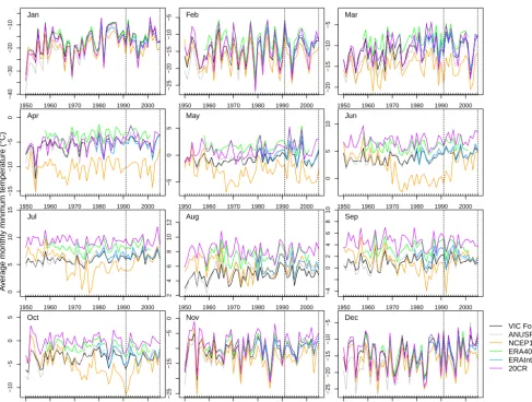
Figure 4. Monthly average minimum temperature by gridded observations (VIC Forcings and ANUSPLIN) and reanalysis (NCEP1, ERA40,

ERAInt, 20CR) over the Peace River basin.

to August. 20CR stands apart from the other reanalyses and both gridded observations with consistently larger precipita-tion amounts, roughly twice the magnitude as observaprecipita-tions in September through to April. However, sequencing of events is similar between 20CR and observations.

This confirms that near surface temperature and precipita-tion values from the selected reanalyses have different char-acteristics due to their different resolutions, model physics, and contributing data in the Peace River basin. The two grid-ded observations also displayed some dissimilarity in time. Differences between these four reanalyses in this particular region should act as a stringent test of the downscaling tech-niques applied. However, we expect that the time-dependent differences between gridded observations and NCEP1 for minimum and maximum temperature, and precipitation, will reduce the success rate of any of the downscaling techniques (Maurer et al., 2013). Nevertheless, we carry NCEP1 through the analysis to quantify the impacts of using a potentially flawed reanalysis and also to evaluate VIC Forcings and

ANUSPLIN over their full record (1950–2005) with two re-analyses (NCEP1 and 20CR).

4.2 Impact of the downscaling approach and reanalyses on ClimDEX results

Downscaled minimum temperature, maximum temperature, and precipitation from seven gridded downscaling methods, two gridded observations, and four reanalyses were used to generate 26 ClimDEX indices. Results were compared to the indices generated from the respective gridded observations at their native resolution (VIC Forcings (∼6 km) and ANUS-PLIN (∼10 km)) for their ability to match the timing (Pear-son’s correlation) and distribution (KS test) of values over the Peace River basin using the Walker field significance test (Wilks, 2006).

(Ta-Table 5. Mean annual ClimDEX values for VIC Forcings and ANUSPLIN averaged over the Peace River basin.

Index Calibration (1950–1990) Validation (1991–2005) Units Indicator name

VIC Forcings ANUSPLIN VIC Forcings ANUSPLIN

cdd 20 19 18 19 Days Consecutive dry days

csdi 5 9 5 6 Days Cold spell duration

cwd 9 10 11 12 Days Consecutive wet days

dtr 11 11 10.6 10.3 ◦C DiurnalT range

fd 239 238 233 230 Days Frost days

gsl 136 131 140 138 Days Growing season

id 109 122 102 106 Days Ice days

prcptot 703 578 742 585 mm Annual total wet-day

r1mm 133 142 150 153 Days Precipitation days

r10mm 17 8 17 8 Days Heavy prec. days

r20mm 4 1 4 1 Days Very heavy prec.

r95p 145 97 142 100 mm Very wet days

r99p 42 28 38 32 mm Extremely wet days

rx1day 32 22 31 23 mm Max 1-day prec.

rx5day 63 46 64 46 mm Max 5-day prec.

sdii 5 4 5 4 mm day−1 Simple daily intense

su 7 6 7 7 Days Summer days

tn10p 11 13 7 8 % Cool nights

tn90p 10 9 12 14 % Warm nights

tnn −37 −41 −35.5 −37.6 ◦C Min monthly Tn

tnx 11 11 11.5 11.8 ◦C Max monthly Tn

tx10p 11 11 9 8 % Cool days

tx90p 10 10 11 14 % Warm days

txn −27 −29 −24.9 −25.8 ◦C Min monthly Tx

txx 27 27 27.9 27.4 ◦C Max monthly Tx

wsdi 4 5 8 12 Days Warm spell duration

ble 5), Namely, PRCPTOT, annual total wet day precipi-tation (>1 mm), in ANUSPLIN is 18 and 21 % less than VIC Forcings in the calibration and validation periods, re-spectively. The events on a given day are larger in VIC Forcings than ANUSPLIN as shown by the higher R95p, RX1day, RX5day, R10mm, and R20mm values. Between the validation and the calibration period, PRCPTOT increases more in VIC Forcings than in ANUSPLIN. The increase in VIC Forcings comes from an increase in precipitation days (R1mm) rather than an increase in intensity. Magni-tudes of the larger precipitation events actually decrease for VIC Forcings, while they increase for ANUSPLIN, although these events are still larger in VIC Forcings than ANUSPLIN in the validation period. The percentage of cool nights de-creases and the duration of warm spells inde-creases somewhat equally for both gridded observations. However, increases in the percentage of warm days and warm nights, and decreases in the percentage of cool days and duration of cold spells, are greater in ANUSPLIN than VIC Forcings, which suggests that the warming signal in ANUSPLIN is stronger. Statisti-cally significant increases in annual minimum temperatures were found by Rodenhuis et al. (2009) in this region. Dif-fering trends in climate extremes are common in gridded ob-servations due to differences in stations, interpolation

tech-niques, and potential corrections for temporal inhomogene-ity. Donat et al. (2014) found that decadal trends in maxi-mum 5-day precipitation amounts (Rx5day) over 1979–2008 ranged from−15 to 5 mm decade−1in the Peace River basin region, depending on the gridded observations they studied. VIC Forcings included a monthly temporal adjustment to in-crease homogeneity (Hamlet and Lettenmaier, 2005), while ANUSPLIN did not. Additionally, stations were allowed to drop in and out on a daily bases in ANUSPLIN, whereas sta-tions had to be available for a minimum of 1 year of consec-utive days and 5 years over the record to be included in VIC Forcings. Hence, trends in some climate extremes differ for these gridded observations and may or may not match those of “reality” and/or reanalyses.

1950 1960 1970 1980 1990 2000

−25

−15

−5

0 Jan

1950 1960 1970 1980 1990 2000

−15

−10

−5

0

5

Feb

1950 1960 1970 1980 1990 2000

−5

0

5

Mar

1950 1960 1970 1980 1990 2000

−5

0

5

10

Apr

1950 1960 1970 1980 1990 2000

51

0

1

5

2

0

May

1950 1960 1970 1980 1990 2000

5

1

01

52

02

5

Jun

1950 1960 1970 1980 1990 2000

10

15

20

25 Jul

1950 1960 1970 1980 1990 2000

10

15

20

25 Aug

1950 1960 1970 1980 1990 2000

51

0

1

5

2

0

Sep

1950 1960 1970 1980 1990 2000

05

1

0 Oct

1950 1960 1970 1980 1990 2000

−15

−10

−5

0

5

Nov

1950 1960 1970 1980 1990 2000

−15

−10

−5

0 Dec

VIC Forcings ANUSPLIN NCEP1 ERA40 ERAInt 20CR

A

v

e

ra

g

e

mo

n

th

ly

ma

x

im

u

m

te

m

p

e

ra

tu

re

(

°C

)

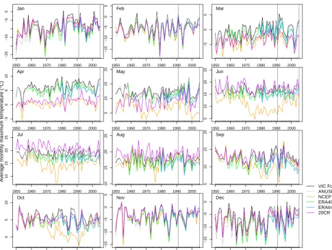
Figure 5. Monthly average maximum temperature by gridded observations (VIC Forcings and ANUSPLIN) and reanalysis (NCEP1, ERA40,

ERAInt, 20CR) over the Peace River basin.

averages of all of the VIC Forcings or ANUSPLIN cells in the Peace basin, while the significance of results was based on the Walker field significance of the correlation tested on each grid cell in the basin.) The largest differences in the number of tests passed primarily occur for precipita-tion based indices where ANUSPLIN passes more than VIC Forcings. VIC Forcings passes 29 more tests than ANUS-PLIN for DTR (Table 7). This result is not unexpected be-cause the differences between the calibration and the vali-dation period are precipitation related in VIC Forcings and temperature related in ANUSPLIN (Table 5). Step changes in daily temperature range (DTR) from 1950 to 2005 are appar-ent in ANUSPLIN (Fig. 8). DTR is a strong driver of snow-pack generation and melt, and errors in simulating realistic DTR could affect hydrologic modelling results.

The sequencing of precipitation indices, such as CWD, PRCPTOT, R10mm, R20mm, R95p, R99p, Rx1day, Rx5day, and SDII, is most difficult to replicate for all methods, espe-cially under VIC Forcings. VIC Forcings has a higher station density than ANUSPLIN because it includes stations from

ob-1950 1960 1970 1980 1990 2000

50

100

150

Jan

1950 1960 1970 1980 1990 2000

50

100

150 Feb

1950 1960 1970 1980 1990 2000

50

100

150 Mar

1950 1960 1970 1980 1990 2000

50

100

150 Apr

1950 1960 1970 1980 1990 2000

0

50

100

150

May

1950 1960 1970 1980 1990 2000

50

100

200

300 Jun

1950 1960 1970 1980 1990 2000

50

100

150

200

Jul

1950 1960 1970 1980 1990 2000

0

50

100

150

200 Aug

1950 1960 1970 1980 1990 2000

0

50

100

150

200

Sep

1950 1960 1970 1980 1990 2000

50

100

150

Oct

1950 1960 1970 1980 1990 2000

0

50

100

150

200 Nov

1950 1960 1970 1980 1990 2000

50

100

150

200 Dec

VIC Forcings ANUSPLIN NCEP1 ERA40 ERAInt 20CR

T

o

ta

l mo

n

th

ly

pr

e

c

ip

it

a

ti

o

n

(

m

m

)

Figure 6. Monthly total precipitation by gridded observations (VIC Forcings and ANUSPLIN) and reanalysis (NCEP1, ERA40, ERAInt,

20CR) over the Peace River basin.

servations to calibrate statistical downscaling methods (Gut-mann et al., 2014; Livneh et al., 2013; Maurer et al., 2002).

Considering results for all downscaling methods and both gridded observations, results based on ERAInt had the high-est score of all four reanalyses for the Pearson correlation and KS tests combined (Table 6). ERAInt results matched sequencing of events most often, as indicated by frequent rejection of the null hypothesis for the Pearson correlation test (Fig. 7; Table 8), and ERA40 results matched distribu-tions most often according to the KS test (Fig. 9; Table 8). The zero-correlation null hypothesis was rejected when com-paring ERAInt for the ANUSPLIN and VIC Forcings grid-ded observations for the number of heavy precipitation days (R10mm), but was not rejected with other reanalyses (Fig. 7). ERA40 and ERAInt monthly average minimum and maxi-mum temperature and total precipitation matched those of the gridded observations most closely (see Sect. 4.1). ERAInt is the highest resolution (1.5◦_{) and both ERAInt and ERA40}

excluded 1950–1958 in their calibration when NCEP1 and 20CR did not (Table 2), which may have avoided potential

combina-Table 6. Summary of the number of tests passed for Pearson’s

corre-lations and similarity in distributions (KS test) based on the Walker field significance test between ClimDEX indices for downscaled reanalyses versus target gridded observation over the Peace River basin for 1991–2005 (1991–2001 ERA40), summarized by gridded observation, reanalysis, and the downscaling method. Max indicates the maximum possible tests to pass in that category.

Pearson’s correlation KS test Combined

Gridded observation

VIC Force 367 578 945

ANUSPLIN 388 628 1016

Max 728 728 1456

Pearson’s correlation KS test Combined

Reanalyses

NCEP1 159 284 443

20CR 147 287 434

ERA40 201 340 541

ERAInt 248 295 543

Max 364 364 728

Pearson’s correlation KS test Combined

Downscaling method

BCCA 130 171 301

DBCCA 139 174 313

BCCI 131 176 307

CI 139 154 293

BCSD 56 175 231

BCSDX 48 173 221

BCCAQ 112 183 295

Max 208 208 416

tion with changes in the gridded observations over 1950– 2005 have resulted in fewer passed tests for 20CR than ERA40 or ERAInt. Thus, choice of reanalysis, calibration period, and the gridded observation data set can influence the measured success of the downscaling approach being tested, irrespective of the method’s inherent strengths and weak-nesses.

The highest ranked downscaling method based on the combined results for field significance of Pearson’s correla-tion and the KS test for all gridded observacorrela-tions, reanaly-ses, and ClimDEX indices was DBCCA (Table 6). It tied for highest rank with CI for correlation, while BCCAQ super-seded all other methods for distribution. Bias remains in re-sults of the BCCA method for precipitation due to the linear combination of fine-scale analogues and uncorrected “driz-zle” and related biases (Guttmann et al., 2014). All down-scaling methods, except CI, include a quantile mapping bias correction step and are expected to do well in matching distri-butions with their respective gridded observation. All meth-ods except CI pass 86 % or more of the tests for

distribu-Table 7. Number of tests passed for each ClimDEX index for VIC

Forcings and ANUSPLIN for 1991–2005 (1991–2001 in ERA40).

VIC Forcings ANUSPLIN Difference

cdd 48 44 4

csdi 54 54 0

cwd 19 31 −12

dtr 32 3 29

fd 51 48 3

gsl 54 52 2

id 55 47 8

prcptot 24 33 −9

r10mm 28 31 −3

r1mm 24 36 −12

r20mm 26 42 −16

r95p 11 28 −17

r99p 24 41 −17

rx1day 14 35 −21

rx5day 30 33 −3

sdii 2 15 −13

su 51 50 1

tn10p 52 52 0

tn90p 48 43 5

tnn 42 39 3

tnx 30 32 −2

tx10p 52 52 0

tx90p 50 50 0

txn 43 44 −1

txx 41 42 −1

wsdi 40 39 1

tion (KS test), while CI passes 78 %. The correlation of DTR was a problem for all the downscaling methods and both gridded observations (Fig. 8) and for distribution based on ANUSPLIN (except BCCAQ), but not when based on VIC Forcings. BCCAQ in combination with ANUSPLIN matched DTR distributions for ERAInt, ERA40, and 20CR when all other methods failed, which points to the success of its ap-proach of post-processing BCCA with a final quantile map-ping bias correction based on BCCI. As mentioned above, DTR is an important driver in snowpacks. Additionally, it plays a key role in evaporation (Sheffield et al., 2012). Rates of evaporation are an important component of projecting fu-ture water availability and drought (Sherwood and Fu, 2014). Therefore, accurately downscaling DTR should be a priority. Including minimum and maximum monthly temperature pre-dictors in BCSDX did not improve the correlation of DTR as was hypothesized in previous studies (Bürger et al., 2012a).

4.3 Impact of the downscaling approach and reanalyses on hydrologic extremes

ex-Table 8. Summary of the number of tests passed for Pearson’s correlations and similarity in distributions (KS test) based on the Walker

field significance test between ClimDEX indices for downscaled reanalyses versus target gridded observation over the Peace River basin for 1991–2005 (1991–2001) for reanalysis (ERA40) versus the downscaling method for each gridded observation.

Pearson’s correlation KS test

NCEP1 20CR ERA40 ERAInt Sub NCEP1 20CR ERA40 ERAInt Sub Total

VIC

F

orcings

BCCA 14 14 14 17 59 19 21 24 18 82 141

DBCCA 15 14 15 18 62 20 22 24 18 84 146

BCCI 14 14 16 20 64 20 21 24 22 87 151

CI 13 14 17 22 66 16 14 24 18 72 138

BCSD 4 6 6 12 28 20 20 24 20 84 112

BCSDX 4 5 7 11 27 20 20 24 20 84 111

BCCAQ 15 13 14 19 61 20 21 24 20 85 146

Subtotal 79 80 89 119 135 139 168 136

ANUSPLIN

BCCA 17 11 23 20 71 22 23 24 20 89 160

DBCCA 17 13 23 24 77 21 20 24 25 90 167

BCCI 14 12 18 23 67 21 21 24 23 89 156

CI 15 14 20 24 73 15 19 24 24 82 155

BCSD 5 4 8 11 28 24 21 25 21 91 119

BCSDX 3 3 5 10 21 24 20 25 20 89 110

BCCAQ 9 10 15 17 51 22 24 26 26 98 149

Subtotal 80 67 112 129 149 148 172 159

ERAInt ERA40 20CR NCEP

bcca

ERAInt ERA40 20CR NCEP

dbcca

ERAInt ERA40 20CR NCEP

bcci

ERAInt ERA40 20CR NCEP

ci

ERAInt ERA40 20CR NCEP

bcsd

ERAInt ERA40 20CR NCEP

bcsdx

ERAInt ERA40 20CR NCEP

cdd csdi cwd dtr fd gsl id prcpto

t

r10mm r1mm r20mm r95p r99p rx1da

y

rx5da

y

sdii su tn10p tn90p tnn tnx tx10p tx90p txn txx wsdi bccaq

bcca

dbcca

bcci

ci

bcsd

bcsdx

cdd csdi cwd dtr fd gsl id prcpto

t

r10mm r1mm r20mm r95p r99p rx1da

y

rx5da

y

sdii su tn10p tn90p tnn tnx tx10p tx90p txn txx wsdi bccaq

Figure 7. Field significant correlations based on the Walker field

significance test over the Peace River basin between ClimDEX in-dices for downscaled reanalysis versus target gridded observation, VIC Forcings (left) and ANUSPLIN (right), by the downscaling method for 1991–2005 (1991–2001 ERA40). Dark grey boxes indi-cate cases in which the null hypothesis is rejected at the 5 % signif-icance level.

tremes when calibrated to one gridded observation versus another. NCEP1 has routinely been used to compare the per-formance of statistical downscaling methods in terms of cli-mate and hydrologic extremes (e.g. Bürger et al., 2012a and Maurer et al., 2010). We thus continue our comparison of multiple gridded observations, reanalyses, and downscaling techniques for hydrologic extremes. Results are compared for 15 years from 1991 to 2005 (inclusive) for the five sub-basins, except for ERA40 (11 years; 1991–2001). We evalu-ate methods for their ability to replicevalu-ate the timing (Pearson’s correlation) and distribution (KS test) of the 3-day peak flow, 7-day low flow in summer, and 7-day low flow in winter.

precip-1950 1960 1970 1980 1990 2000

9

1

01

11

21

3

dtr vicforce NCEP

Year

T

emper

ature (

°

C)

1950 1960 1970 1980 1990 2000

9

1

01

11

21

3

dtr vicforce 20CR

Year

T

emper

ature (

°

C)

1950 1960 1970 1980 1990 2000

9

1

01

11

21

3

dtr vicforce ERA40

Year

T

emper

ature (

°

C)

1950 1960 1970 1980 1990 2000

9

1

01

11

21

3

dtr vicforce ERAInt

Year

T

emper

ature (

°

C)

1950 1960 1970 1980 1990 2000

9

1

01

11

21

3

dtr anusplin NCEP

Year

T

emper

ature (

°

C)

1950 1960 1970 1980 1990 2000

9

1

01

11

21

3

dtr anusplin 20CR

Year

T

emper

ature (

°

C)

1950 1960 1970 1980 1990 2000

9

1

01

11

21

3

dtr anusplin ERA40

Year

T

emper

ature (

°

C)

1950 1960 1970 1980 1990 2000

9

1

01

11

21

3

dtr anusplin ERAInt

Year

T

emper

ature (

°

C)

gridobs bcca dbcca bcci ci bcsd bcsdx bccaq

Figure 8. Time series of average DTR from VIC Forcings (left) and ANUSPLIN (right) for NCEP1 (top), 20CR (second), ERA40 (third),

and ERAInt (bottom) downscaled using BCCA, DBCCA, BCCI, CI, BCSD, BCSDX, and BCCAQ over the Peace River basin.

itation is less representative than VIC Forcings. Out of the two statistical tests and three metrics the only case where ANUSPLIN passed more tests than VIC Forcings was for correlation in summer 7-day low flow (Table 10), especially when driven with NCEP1 and 20CR downscaled via BCCA and DBCCA. Similar results were found for ANUSPLIN and BCCA and DBCCA with the ClimDEX indices (Sect. 4.2).

This suggests that there is potential for ClimDEX results to act as a predictor of hydrologic extremes.

val-ERAInt ERA40 20CR NCEP

bcca

ERAInt ERA40 20CR NCEP

dbcca

ERAInt ERA40 20CR NCEP

bcci

ERAInt ERA40 20CR NCEP

ci

ERAInt ERA40 20CR NCEP

bcsd

ERAInt ERA40 20CR NCEP

bcsdx

ERAInt ERA40 20CR NCEP

cdd csdi cwd dtr fd gsl id prcpto

t

r10mm r1mm r20mm r95p r99p rx1da

y

rx5da

y

sdii su tn10p tn90p tnn tnx tx10p tx90p txn txx wsdi bccaq

bcca

dbcca

bcci

ci

bcsd

bcsdx

cdd csdi cwd dtr fd gsl id prcpto

t

r10mm r1mm r20mm r95p r99p rx1da

y

rx5da

y

sdii su tn10p tn90p tnn tnx tx10p tx90p txn txx wsdi bccaq

Figure 9. Field significant similarities in distributions based on the

Walker field significance test over the Peace River basin between ClimDEX indices for downscaled reanalysis versus target gridded observation, VIC Forcings (left), and ANUSPLIN (right), by the downscaling method for 1991–2005 (1991–2001 ERA40). Dark grey boxes indicate cases in which the null hypothesis is not re-jected at the 5 % significance level.

idation period for ERA40, 1990–2001 versus 1990–2005 for other reanalyses, could have avoided some challenging hy-drologic extreme events in 2002–2005. However, ERAInt, which was validated over 1990–2005, passed nearly the same number of tests as ERA40. Thus, the shorter calibration pe-riod in ERA40 and ERAInt avoids step changes in the grid-ded observations and reanalyses prior to 1958. Peculiarities with the gridded observations were apparent from 1950 to 1958 for the monthly average minimum and maximum tem-peratures (Figs. 4 and 5) and for the DTR and SDII ClimDEX indices (Figs. 8 and 10). Avoiding these years could have reduced artefacts in the downscaled products and hydro-logic model results. Nevertheless, many studies have demon-strated that ERA40 and ERAInt are superior products ver-sus NCEP1 (Donat et al., 2014; Ma et al., 2008, 2009; Sill-mann et al., 2013a). In our own analysis ERA40 and ERAInt have similar timing and magnitude in minimum and maxi-mum temperature and precipitation (Figs. 4, 5, and 6) to the gridded observations when NCEP1 and 20CR do not. These results confirm that downscaling methods will succeed when applied to reanalyses that have correct timing, magnitude, and trends such as ERA40 and ERAInt, more so than when applied to reanalyses such as NCEP1 and 20CR that have ir-regular step changes (Maraun, 2013). We should be able to assume that although the biases in GCMs will be greater than

Table 9. Summary of the number of tests passed for Pearson’s

corre-lations and similarity in distributions (KS test) based on the Walker field significance test between hydrologic extremes for downscaled reanalyses versus target gridded observation over the Peace basin for 1991–2005 (1991–2001 ERA40), summarized by gridded ob-servation, reanalysis, and downscaling method. Max indicates the maximum possible tests to pass in that category.

Pearson’s correlation KS test Combined

Gridded observation

VIC Force 309 404 713

ANUSPLIN 310 350 660

Max 420 420 840

Pearson’s correlation KS test Combined

Reanalyses

NCEP1 135 188 323

20CR 125 181 306

ERA40 180 196 376

ERAInt 179 189 368

Max 210 210 420

Pearson’s correlation KS test Combined

Downscaling method

BCCA 102 96 198

DBCCA 104 111 215

BCCI 107 111 218

CI 99 87 186

BCSD 49 119 168

BCSDX 48 119 167

BCCAQ 110 111 221

Max 120 120 240

those found in reanalyses, they are consistent over time. The strength of downscaling methods when downscaling ERA40 and ERAInt versus NCEP1 and 20CR was also found with the ClimDEX indices.

Table 10. Number of basins where the null hypothesis that the downscaled and observed (VIC Forcings and ANUSPLIN) derived 3-day peak

flows are not linearly correlated was rejected and the number of basins where the null hypothesis that the downscaled and observed based distributions are drawn from the same sample was not rejected, by downscaling method/reanalysis combinations for 1991–2005 (1991–2001 ERA40).

Pearson’s correlation KS test

NCEP1 20CR ERA40 ERAInt Sub NCEP1 20CR ERA40 ERAInt Sub Total

VIC

F

orcings

BCCA 2 2 5 5 14 5 5 5 1 16 30

DBCCA 1 3 5 5 14 5 5 5 5 20 34

BCCI 2 5 5 5 17 5 5 5 5 20 37

CI 5 2 5 5 17 5 5 5 5 20 37

BCSD 3 2 4 2 11 5 5 5 5 20 31

BCSDX 3 3 4 2 12 5 5 5 5 20 32

BCCAQ 3 5 5 5 18 5 5 5 5 20 38

Subtotal 19 22 33 29 103 35 35 35 31 136

ANUSPLIN

BCCA 5 0 5 5 15 4 4 4 1 13 28

DBCCA 5 1 5 5 16 5 2 4 5 16 32

BCCI 5 2 4 5 16 5 2 4 5 16 32

CI 4 0 5 5 14 5 2 4 5 16 30

BCSD 2 0 3 3 8 5 5 5 5 20 28

BCSDX 2 0 3 3 8 5 5 4 5 19 27

BCCAQ 5 3 5 5 18 5 2 5 5 17 35

Subtotal 28 6 30 31 95 34 22 30 31 117

from BCCI (Maraun, 2013) and largely corrects remnant bi-ases in magnitude from BCCA (Guttmann et al., 2014). Spa-tial covariability is much more relevant in hydrologic mod-elling than the comparison of climate indices between prod-ucts on a grid cell to grid cell basis. This method is also better at maintaining long-term trends, which might explain failed tests in some of the sub-basins when downscaling NCEP1 and 20CR, which, as shown earlier, exhibit inhomogeneities between calibration and validation periods. BCCAQ could be failing for the “right reason” when the trend in VIC Forcings or ANUSPLIN for a given metric is opposite that in NCEP1 or 20CR. BCCAQ is the only method to pass the Pearson cor-relation and KS test in all five sub-basins when downscaling ERA40 or ERAInt to VIC Forcings or ANUSPLIN for all three hydrologic extremes. BCCAQ has overcome some of the challenges of BCCA that Maurer et al. (2010) would not have been able to find using NCEP1 alone as surrogate GCM. It is also more successful than the BCCI method, which is analogous to the statistical downscaling and bias correction (SDBC) method in Ahmed et al. (2013) and asynchronous re-gression (AR) in Gutmann et al. (2014), by avoiding overesti-mates of extreme events at aggregate scales (Maraun, 2013). The BCSD methods pass the most tests for distribution for all basins and reanalyses, while they fail more tests than any other downscaling method for correlation due to their re-liance on random sampling of historical months when tempo-rally disaggregating from the monthly to daily time step (Ta-ble 6). Thus, these methods will get the frequency and mag-nitude of events correct, but will get the timing of when these

rain-on-1950 1960 1970 1980 1990 2000

34567

sdii vicforce NCEP

Year

mm da

y~−1

1950 1960 1970 1980 1990 2000

34567

sdii vicforce 20CR

Year

mm da

y~−1

1950 1960 1970 1980 1990 2000

34567

sdii vicforce ERA40

Year

mm da

y~−1

1950 1960 1970 1980 1990 2000

34567

sdii vicforce ERAInt

Year

mm da

y~−1

1950 1960 1970 1980 1990 2000

34567

sdii anusplin NCEP

Year

mm da

y~−1

1950 1960 1970 1980 1990 2000

34567

sdii anusplin 20CR

Year

mm da

y~−1

1950 1960 1970 1980 1990 2000

34567

sdii anusplin ERA40

Year

mm da

y~−1

1950 1960 1970 1980 1990 2000

34567

sdii anusplin ERAInt

Year

mm da

y~−1

gridobs bcca dbcca bcci ci bcsd bcsdx bccaq

Figure 10. Time series of average SDII from VIC Forcings (left) and ANUSPLIN (right) for NCEP1 (top), 20CR (second), ERA40 (third),

and ERAInt (bottom) downscaled using BCCA, DBCCA, BCCI, CI, BCSD, BCSDX, and BCCAQ over the Peace River basin.

snow events caused by the downscaling-driven results that are not displayed in the runs based on gridded observations. The CI method is the closest to the delta method that we have investigated. The median and ranges for CI are much lower for winter 7-day low flow (not shown). The poorer

base bcca _dbcca bcci

ci

bcsd _{bcsdx bccaq}

2000 3000 4000 5000 6000 7000 BCGMS NCEP1

1992 1996 2000 2004

2000

4000

6000

BCGMS NCEP1

Year

2000 3000 4000 5000 6000 7000

0.0 0 .4 0.8 BCGMS NCEP1 m3 s

base bcca _dbcca bcci

ci

bcsd _{bcsdx bccaq}

2000 3000 4000 5000 6000 7000 BCGMS 20CR

1992 1996 2000 2004

2000

4000

6000

BCGMS 20CR

Year

2000 3000 4000 5000 6000 7000

0.0 0 .4 0.8 BCGMS 20CR m3 s

base bcca _dbcca bcci

ci

bcsd _{bcsdx bccaq}

2000 3000 4000 5000 6000 7000 BCGMS ERA40

1992 1996 2000 2004

2000

4000

6000

BCGMS ERA40

Year

2000 3000 4000 5000 6000 7000

0.0 0 .4 0.8 BCGMS ERA40 m3 s

base bcca _dbcca bcci

ci

bcsd _{bcsdx bccaq}

2000 3000 4000 5000 6000 7000 BCGMS ERAInt

1992 1996 2000 2004

2000

4000

6000

BCGMS ERAInt

Year

2000 3000 4000 5000 6000 7000

0.0 0 .4 0.8 BCGMS ERAInt m3 s base bcca dbcca bcci ci

bcsd _{bcsdx bccaq}

2000 3000 4000 5000 6000 7000 BCGMS NCEP1

1992 1996 2000 2004

2000

4000

6000

BCGMS NCEP1

Year

2000 3000 4000 5000 6000 7000

0.0 0.4 0.8 BCGMS NCEP1 m3 s base bcca dbcca bcci ci

bcsd _{bcsdx bccaq}

2000 3000 4000 5000 6000 7000 BCGMS 20CR

1992 1996 2000 2004

2000

4000

6000

BCGMS 20CR

Year

2000 3000 4000 5000 6000 7000

0.0 0.4 0.8 BCGMS 20CR m3 s base bcca dbcca bcci ci

bcsd _{bcsdx bccaq}

2000 3000 4000 5000 6000 7000 BCGMS ERA40

1992 1996 2000 2004

2000

4000

6000

BCGMS ERA40

Year

2000 3000 4000 5000 6000 7000

0.0 0.4 0.8 BCGMS ERA40 m3 s base bcca dbcca bcci ci

bcsd _{bcsdx bccaq}

2000 3000 4000 5000 6000 7000 BCGMS ERAInt

1992 1996 2000 2004

2000

4000

6000

BCGMS ERAInt

Year

2000 3000 4000 5000 6000 7000

0.0 0.4 0.8 BCGMS ERAInt m3 s –1 –1 –1 –1 –1 –1 –1 –1 –1 –1 –1 –1

Figure 11. Boxplots, time series, and distributions of 3-day peak flow in the spring months (May–July) for NCEP1, 20CR, ERA40, and

Table 11. As in Table 10 but for summer 7-day low flow.

Pearson’s correlation KS test

NCEP1 20CR ERA40 ERAInt Sub NCEP1 20CR ERA40 ERAInt Sub Total

VIC

F

orcings

BCCA 3 2 5 5 15 5 5 5 5 20 35

DBCCA 3 2 5 5 15 5 5 5 5 20 35

BCCI 3 4 5 5 17 5 5 5 5 20 37

CI 2 4 5 5 16 5 5 5 5 20 36

BCSD 2 3 3 4 12 5 5 5 5 20 32

BCSDX 2 2 3 4 11 5 5 5 5 20 31

BCCAQ 4 3 5 5 17 5 5 5 5 20 37

Subtotal 19 20 31 33 103 35 35 35 35 140

ANUSPLIN

BCCA 5 4 5 5 19 5 5 5 1 16 35

DBCCA 5 5 5 5 20 5 5 5 5 20 40

BCCI 3 5 5 5 18 5 5 5 5 20 38

CI 1 5 5 5 16 5 5 5 5 20 36

BCSD 1 2 4 5 12 5 5 5 5 20 32

BCSDX 1 2 4 5 12 5 5 5 5 20 32

BCCAQ 3 5 5 5 18 5 5 5 5 20 38

Subtotal 19 28 33 35 115 35 35 35 31 136

1992 1996 2000 2004

200

600

1000

1400

BCGMS NCEP1

Year

1992 1996 2000 2004

200

600

1000

1400

BCGMS 20CR

Year

1992 1996 2000 2004

200

600

1000

1400

BCGMS ERA40

Year

1992 1996 2000 2004

200

600

1000

1400

BCGMS ERAInt

Year

1992 1996 2000 2004

200

600

1000

1400

BCGMS NCEP1

Year

1992 1996 2000 2004

200

600

1000

1400

BCGMS 20CR

Year

1992 1996 2000 2004

200

600

1000

1400

BCGMS ERA40

Year

1992 1996 2000 2004

200

600

1000

1400

BCGMS ERAInt

Year

Figure 12. Time series of 7-day low flow in the summer months (July–September) for NCEP1, 20CR, ERA40, and ERAInt in the BCGMS

basin based on VIC Forcings (top) and ANUSPLIN (bottom). Legend same as Fig. 9.

5 Conclusions

We have tested the applicability of seven techniques for downscaling coarse-scale climate models in terms of ClimDEX indices and hydrologic extremes. The seven ap-proaches investigated include several methods commonly used in hydrologic modelling. Some of these had been ex-plored before (i.e. BCSD and BCCA), but not using mul-tiple reanalyses. Choice of reanalysis was found to affect the number of tests passed for a given downscaling tech-nique. Downscaling methods were more successful under ERA40 or ERAInt than they were under NCEP1 or 20CR.

Table 12. As in Table 10 but for winter 7-day low flow.

Pearson’s correlation KS test

NCEP1 20CR ERA40 ERAInt Sub NCEP1 20CR ERA40 ERAInt Sub Total

VIC

F

orcings

BCCA 5 5 5 5 20 5 5 5 5 20 40

DBCCA 5 5 5 5 20 5 5 5 5 20 40

BCCI 5 5 5 5 20 5 5 5 5 20 40

CI 5 5 4 5 19 4 2 2 0 8 27

BCSD 0 0 2 0 2 5 5 5 5 20 22

BCSDX 0 0 2 0 2 5 5 5 5 20 22

BCCAQ 5 5 5 5 20 5 5 5 5 20 40

Subtotal 25 25 28 25 103 34 32 32 30 128

ANUSPLIN

BCCA 5 5 4 5 19 1 3 4 3 11 30

DBCCA 5 5 4 5 19 2 3 5 5 15 34

BCCI 5 4 5 5 19 2 3 5 5 15 34

CI 5 5 3 4 17 0 0 0 3 3 20

BCSD 0 0 2 2 4 4 5 5 5 19 23

BCSDX 0 1 2 0 3 5 5 5 5 20 23

BCCAQ 5 4 5 5 19 1 3 5 5 14 33

Subtotal 25 24 25 26 100 15 22 29 31 97

1992 1996 2000 2004

100

300

500

BCGMS NCEP1

Year

1992 1996 2000 2004

100

300

500

BCGMS 20CR

Year

1992 1996 2000 2004

100

300

500

BCGMS ERA40

Year

1992 1996 2000 2004

100

300

500

BCGMS ERAInt

Year

1992 1996 2000 2004

100

300

500

BCGMS NCEP1

Year

1992 1996 2000 2004

100

300

500

BCGMS 20CR

Year

1992 1996 2000 2004

100

300

500

BCGMS ERA40

Year

1992 1996 2000 2004

100

300

500

BCGMS ERAInt

Year

Figure 13. Time series of 7-day low flow in the winter months (November–April) for NCEP1, 20CR, ERA40, and ERAInt in the BCGMS

basin based on VIC Forcings (top) and ANUSPLIN (bottom). Legend same as Fig. 9.

this work we learned a lot about these gridded observations and discovered evaluation procedures that will be useful for future studies.

BCSDX, DBCCA, and BCCAQ downscaling methods had not been evaluated in terms of ClimDEX indices and hydro-logic extremes before now. The BCSDX method included minimum and maximum temperature from the reanalyses in-stead of mean as is done in BCSD, but this did not improve its ability to resolve temperature indices, such as diurnal tem-perature range or hydrologic extremes. DBCCA was an im-provement over BCCA and passed the greatest number of tests for the ClimDEX indices. The double bias correction