Positive Impact Program Evaluation

(1)

Physics and Astronomy Dissertations Department of Physics and Astronomy

Spring 4-2-2012

Spectroscopy and Interferometry of the Winds of Luminous Blue

Variables

Noel D. Richardson

Center for High Angular Resolution Astronomy

Follow this and additional works at: https://scholarworks.gsu.edu/phy_astr_diss

Recommended Citation Recommended Citation

Richardson, Noel D., "Spectroscopy and Interferometry of the Winds of Luminous Blue Variables." Dissertation, Georgia State University, 2012.

https://scholarworks.gsu.edu/phy_astr_diss/52

This Dissertation is brought to you for free and open access by the Department of Physics and Astronomy at ScholarWorks @ Georgia State University. It has been accepted for inclusion in Physics and Astronomy

(2)

by

NOEL DOUGLAS RICHARDSON Under the Direction of Douglas R. Gies

ABSTRACT

Massive stars are rare, but emit most of the light we observe in the Universe and create many of the heavy elements in the Universe. In this dissertation, I explore the winds of the massive luminous blue variable (LBV) stars. New observational approaches and long time-series are utilized in order to examine the basic observable properties of the stars and the mass lost during their lifetimes.

(3)

different amplitudes. Future studies of LBV winds are outlined, as well as a short discussion of Georgia State University’s Hard Labor Creek Observatory for these types of studies. INDEX WORDS: Circumstellar matter, Stars, Emission-line, Be, Winds, Outflows,

(4)

by

NOEL DOUGLAS RICHARDSON

A Dissertation Submitted in Partial Fulfillment of Requirements for the Degree of Doctor of Philosophy

in the College of Arts and Sciences Georgia State University

(5)

(6)

by

NOEL DOUGLAS RICHARDSON

Committee Chair:

Committee:

Douglas R. Gies

Harold A. McAlister

Todd J. Henry

Misty C. Bentz

Brian D. Thoms

Nancy D. Morrison

Electronic Version Approved:

Office of Graduate Studies

College of Arts and Sciences

Georgia State University

(7)

Dedication

(8)

ACKNOWLEDGMENTS

This dissertation has taken a large effort to collect and analyze the necessary data. I could not have done this without a large amount of support. First, I would like to thank my wonderfully patient wife, Kristy. She has supported me through the large changes that have occurred over the previous six years, kept me on track when I couldn’t see what to do, and listened to me as graduate school caused stress. She was incredibly understanding as I went on observing runs to the CHARA Array or Lowell Observatory, traveled to conferences, or on collaborative trips. I owe much of this work to her support, and could never thank her enough. Her dedication to the final work in this dissertation is fundamentally important, as she often cared for our daughter so I could write.

The rest of my family has also been supportive through this process. My mother encour-aged me through my education, and I wish she were still here so that she would be able to see this final stage. My father has supported me in many ways, and has always listened when I needed to talk. My sisters have been there through it as well, listening to my frustrations and aspirations. During this research, I have gone to Boston twice to work on things with Dan Clemens (BU) and my aunt and uncle in Boston have graciously helped me out at those times by providing a place to stay and transportation while I was there.

Doug Gies has been an extraordinary advisor who has allowed me to shape this disser-tation in my own manner from the beginning. He encouraged me to take on projects and did not ever tell me not to pursue work on LBVs, despite his lack of former experience with these stars. He has supported the projects with grants, time, dedication, and enthusiasm. I cannot thank him enough for that.

(9)

software development issues). Also, Todd Henry encouraged me to apply for SMARTS time, which led to the development of Chapters 4–6 of this dissertation.

Nancy Morrison advised me with my undergraduate and M.S. research at the University of Toledo. The methods she taught me provided a solid basis for this research. Her long-term monitoring projects at Ritter Observatory allowed for the development of Chapter 2, which has interesting aspects of LBV physics from an in-depth study of the wind of P Cygni. I appreciate her advice, her time, and her travel for this dissertation.

Chapter 2 also benefited greatly by the advice and help of several people. Nevena Markova provided many useful comments, as well as her earlier published data on the star (both spectroscopy and photometry). Erica Hesselbach provided new reduced observations of the star made at Ritter Observatory. John Percy provided additional archival photometry and great advice in the early stages of the project.

CHARA observations of P Cygni are shown in Chapter 3. Early CHARA observations of this star developed my interest in LBVs, so special thanks to Peter Tuthill (University of Sydney) and Theo ten Brummelaar for that help. The MIRC observations and analysis presented in Chapter 3 began with the help of Gail Schaefer. Early analysis was performed with her assistance as well as that of John Monnier and Yamina Touhami. Rob Parks performed additional imaging tests at that time. This work continues with help from Fabien Baron. The CHARA Array relies on the additional help of Chris Farrington, P.J. Goldfinger, Sandy Land, Judit Sturmann, Laszlo Sturmann, Nils Turner, and Larry Webster.

(10)

observations, which was certainly difficult with the η Carinae program, and all data were masterfully scheduled.

The η Carinae project (Chapter 4) benefited from advice from Mike Corcoran, Kris Davidson, Ted Gull, Roberta Humphreys, Tom Madura, Krister Nielsen, and Julian Pittard. Roberta Humphreys was also a great help in the early stages of my LBV survey. She provided a few targets that I had overlooked and that are certainly interesting in their own respect.

Some spectra were obtained at GSU’s Hard Labor Creek Observatory. This facility has come a long way over the time I have spent at GSU. Our department chairman, Dick Miller, has certainly been instrumental in these upgrades and improvements. The new 20 inch telescope was also helped along by Hal McAlister. The installation of this telescope was done with the help of Charles Hopper and Nic Scott, with some additional help from the instrument shop, John Wilson, and many other people in the department. The spectrograph saw first light last summer, which was overseen by many of the people already listed in this paragraph. Additional support for that project came from Ben Jenkins, who completed his M.S. thesis with that instrument. However, I must acknowledge Emily Aldoretta who spent her summer and fall semesters learning the instrument and telescope, the data reduction, and performing some analysis for her undergraduate thesis. Her help was instrumental in showing how much work can be done with that telescope and spectrograph.

(11)

(12)

TABLE OF CONTENTS

ACKNOWLEDGMENTS . . . v

LIST OF TABLES . . . xii

LIST OF FIGURES . . . xiii

LIST OF ABBREVIATIONS . . . xviii

1 INTRODUCTION . . . 1

1.1 THE IMPORTANCE OF MASSIVE STARS . . . 1

1.2 STELLAR WINDS . . . 2

1.3 OBSERVABLES OF STELLAR WINDS . . . 3

1.4 TYPES OF STARS MENTIONED IN THIS DISSERTATION . . . 5

1.5 DEFINITION AND THE IMPORTANCE OF LUMINOUS BLUE VARIABLES 5 1.6 BINARIES AND THE LBVS . . . 10

1.7 OUTLINE OF THIS DISSERTATION . . . 13

2 THE Hα VARIATIONS OF THE LUMINOUS BLUE VARIABLE P CYGNI: DISCRETE ABSORPTION COMPONENTS AND THE SHORT S DORADUS PHASE . . . 15

2.1 INTRODUCTION TO P CYGNI . . . 15

2.2 OBSERVATIONS . . . 18

2.3 THE LONG-TERM PHOTOMETRIC AND HαEQUIVALENT WIDTH VARI-ABILITY . . . 19

2.4 Hα PROFILE MORPHOLOGY VARIABILITY . . . 25

2.4.1 Emission Component Changes . . . 25

2.4.2 Blue Absorption Changes . . . 27

2.5 DISCUSSION . . . 36

3 THE ANGULARLY RESOLVED WIND OF P CYGNI . . . 45

3.1 INTRODUCTION AND BASIC THEORY . . . 45

(13)

3.3 IMPLICATIONS OF THE MIRC OBSERVATIONS AND THE LARGE SCALE

STRUCTURE OF P CYGNI’S EJECTA . . . 57

3.4 H-BAND VARIATIONS OF P CYGNI, AND IMPLICATIONS ON THE EMITTING REGION SIZE . . . 61

3.4.1 Spectroscopic H-band Observations . . . 61

3.4.2 H-band Variability . . . 62

4 THE Hα VARIATIONS OF η CARINAE DURING THE 2009.0 SPECTROSCOPIC EVENT . . . 68

4.1 INTRODUCTION TO η CARINAE . . . 68

4.2 OBSERVATIONS . . . 71

4.3 Hα OBSERVATIONS AND VARIABILITY DURING THE 2009.0 SPEC-TROSCOPIC EVENT . . . 73

5 A BINARY ORBIT FOR THE MASSIVE, EVOLVED STAR HDE 326823, A WR+O SYSTEM PROGENITO . . . 88

5.1 INTRODUCTION . . . 88

5.2 PHOTOMETRIC VARIATIONS . . . 90

5.3 SPECTROSCOPIC VARIATIONS . . . 92

5.3.1 Observations . . . 92

5.3.2 Absorption Line Variability . . . 93

5.3.3 A Single-Lined Spectroscopic Orbit . . . 95

5.3.4 Emission Line Variability . . . 97

5.5 SUMMARY . . . 112

6 A THREE YEAR SPECTROSCOPIC SURVEY ON THE VARIABIL-ITY OF GALACTIC AND MAGELLANIC LUMINOUS BLUE VARI-ABLES . . . 114

6.1 INTRODUCTION . . . 114

6.2 OBSERVATIONS AND TARGET STARS . . . 115

6.3 DESCRIPTION OF THE SPECTRA OF LBVS . . . 118

6.4 BACKGROUND AND RESULTS ON TARGET STARS . . . 120

(14)

6.4.2 R 85 . . . 126

6.4.3 S Doradus . . . 131

6.4.4 R 110 . . . 139

6.4.5 R 127 . . . 143

6.4.6 HR Carinae . . . 149

6.4.7 AG Carinae . . . 156

6.4.8 Wra 751 . . . 163

6.4.9 ζ1 _{Sco . . . 168}

6.4.10 HD 160529 . . . 173

6.4.11 HD 168607 . . . 178

6.4.12 HD 168625 . . . 182

6.4.13 V452 Sct = AS 314 . . . 186

6.5 STARS CROSSING THE BISTABILITY JUMP . . . 190

6.6 ON THE VARIABILITY OF THE POPULATION . . . 191

6.7 FUTURE WORK – WHICH LBVS ARE THE BEST TO OBSERVE AND WHY? . . . 194

7 FUTURE WORK . . . 198

7.1 SPECTROSCOPY OF MASSIVE STELLAR WINDS AT HARD LABOR CREEK OBSERVATORY . . . 198

7.2 INTERFEROMETRIC WORK . . . 200

7.3 LUMINOUS BLUE VARIABLES . . . 202

References . . . 205

Appendices . . . 217

A HLCO SPECTROSCOPY REDUCTION . . . 218

A.1 INTRODUCTION . . . 218

A.2 EXTRACTING THE SPECTRA AND WAVELENGTH CALIBRATION . . 218

B MEASUREMENTS . . . 220

(15)

LIST OF TABLES

Table 1.1 Types of Massive, Evolved Stars . . . 5

Table 1.2 Published Orbital Elements of HD 5980 . . . 12

Table 3.1 Infrared Flux Measurements of P Cyg . . . 64

Table 5.1 HDE 326823 N II Radial Velocities . . . 95

Table 5.2 HDE 326823 Spectroscopic Orbit . . . 96

Table 5.3 HDE 326823 He I λ5876 Measurements . . . 101

Table 6.1 Observations collected with SMARTS (RCspec) . . . 116

Table 6.2 Previously Determined Mass-loss rates of Galactic LBVs . . . 120

Table 6.3 Hα Equivalent Width Summary . . . 192

Table A.1 Reduction lists for HLCO . . . 218

Table B.1 Hα Measurements of P Cygni . . . 220

Table B.2 Hα Measurements of η Carinae During the 2009.0 Event . . . 222

Table B.3 Hα Measurements of LBVs . . . 222

(16)

LIST OF FIGURES

Figure 1.1 The P Cygni Profile . . . 4

Figure 1.2 The Upper H-R Diagram . . . 7

Figure 1.3 LBV ejecta . . . 10

Figure 1.4 The geometry of an LBV’s wind . . . 11

Figure 2.1 The Historic Light Curve of P Cygni . . . 16

Figure 2.2 V-band Variability of P Cygni . . . 20

Figure 2.3 Discrete Fourier Transforms of the V-band Photometry . . . 22

Figure 2.4 Hα and V-band co-variations . . . 24

Figure 2.5 Extremes of the Hα Variations . . . 26

Figure 2.6 Long Term Behavior of Hα Profile Properties . . . 28

Figure 2.7 Dynamical Spectrum Showing the Discrete Absorption Components in the Hα Profile of P Cygni . . . 30

Figure 2.8 Progession of a DAC . . . 32

Figure 2.9 Variability of the Blue Absorption Trough . . . 33

Figure 2.10 Velocities of the Absorption Components . . . 35

Figure 2.11 FWHM and Hα Equivalent Width Relation . . . 40

Figure 2.12 The Long Term Behavior of the DACs . . . 42

Figure 3.1 Modeled Spectrophotometry of a Star with a Strong Wind (P Cygni) 47 Figure 3.2 The Effect of a Stellar Wind on a Measured Diameter of a Photosphere 48 Figure 3.3 (u, v) Coverage for MIRC observations of P Cygni . . . 51

Figure 3.4 Visibility Fit to the MIRC observations of P Cygni . . . 53

Figure 3.5 Best fit model to the MIRC data of P Cygni . . . 54

Figure 3.6 Closure Phases Observed for P Cygni . . . 55

Figure 3.7 MACIM image reconstruction of the MIRC data of P Cygni . . . 56

Figure 3.8 MACIM image reconstruction of P Cygni’s wind . . . 58

(17)

Figure 3.10 The wind of P Cygni at multiple scales . . . 60

Figure 3.11 H-band spectrophotometry of P Cygni 2008–2010 . . . 63

Figure 3.12 K-band spectrophotometry of P Cygni 2006–2010 . . . 64

Figure 3.13 Flux errors for Mimir Observations . . . 65

Figure 3.14 Spectrophotometry of P Cygni compared with a model atmosphere . 67 Figure 4.1 The Historic Light Curve of η Car . . . 70

Figure 4.2 The Homunculus Surrounding η Car . . . 71

Figure 4.3 Hα Line Profiles of η Car During the 2009.0 Event . . . 75

Figure 4.4 Logarithmic Gray Scale Representation of the Hα Profile of η Car During the 2009.0 Event . . . 76

Figure 4.5 Hα Variations of η Car During the last two Events . . . 78

Figure 4.6 Hα Equivalent Widths and Photometry of η Car During the 2009.0 Event . . . 79

Figure 4.7 Isothermal Models of the Colliding Winds in the η Car system . . . . 81

Figure 4.8 Hα Radial Velocity Variations of η Car During the 2009.0 Event . . . 84

Figure 5.1 Photometry of HDE 326823 . . . 91

Figure 5.2 Orbitally Modulated N II Profiles . . . 94

Figure 5.3 An Orbit for HDE 326823 . . . 96

Figure 5.4 Orbitally Modulated He I 5876 Line Profiles . . . 98

Figure 5.7 Orbitally Modulated He I 5876 Equivalent Widths . . . 103

Figure 5.8 Orbitally Modulated Hα Line Profiles . . . 104

Figure 5.9 Orbitally Modulated Fe II 6345 Line Profiles . . . 105

Figure 5.10 Graphic Depiction of the Binary System HDE 326823 . . . 108

Figure 6.1 Galactic LBVs . . . 119

Figure 6.2 Magellanic LBVs . . . 121

(18)

Figure 6.4 Line Plots of the Hα Profiles of R 40 . . . 124

Figure 6.5 Photometry and Hα Equivalent Width Variability of R 40 . . . 125

Figure 6.6 Dynamical representation of the Hα Observations of R 85 . . . 127

Figure 6.7 Line Plots of the Hα Profiles of R 85 . . . 128

Figure 6.9 Line Plots for the He I 6678 Observations of R 85 . . . 130

Figure 6.10 Photometry of S Doradus, 1889–2011 . . . 132

Figure 6.11 S Dor in Different Optical States . . . 133

Figure 6.12 Observed Hα profiles of S Doradus . . . 135

Figure 6.13 Fe II emission in S Dor . . . 136

Figure 6.14 Logarithmic representation of the observed Hα profiles of S Doradus . 137 Figure 6.15 Photometry and Hα Equivalent Width Variability of S Doradus . . . 138

Figure 6.16 Dynamical Representation of the Hα profiles of R 110 . . . 140

Figure 6.17 Line Plots of the Hα profiles of R 110 . . . 141

Figure 6.19 Fe II emission in R 127 . . . 144

Figure 6.20 Observed Hα profiles of R 127 . . . 145

Figure 6.21 Dynamical representation of the observed Hα profiles of R 127 . . . . 146

Figure 6.23 He I lines observed in R 127 . . . 148

Figure 6.24 Dynamical Spectrum of the Hα profiles of HR Car . . . 150

Figure 6.25 Observed Line Spectra of the Hα profiles of HR Car . . . 151

Figure 6.26 Photometry and Hα Equivalent Width Variability of HR Car . . . 153

Figure 6.27 Dynamical Spectrum of the He I 6678 profiles of HR Car . . . 154

Figure 6.28 Observed Line Spectra of the He I 6678 profiles of HR Car . . . 155

Figure 6.29 Dynamical Spectrum of the Hα profiles of AG Car . . . 158

Figure 6.30 Observed Line Spectra of the Hα profiles of AG Car . . . 159

Figure 6.31 Photometry and Hα Equivalent Width Variability of AG Car . . . 160

(19)

Figure 6.33 Observed Line Spectra of the He I 6678 profiles of AG Car . . . 162

Figure 6.34 Wra 751 dynamical spectrum . . . 165

Figure 6.35 Wra 751 Hα profiles . . . 166

Figure 6.36 Photometry and Hα Equivalent Width Variability of Wra 751 . . . . 167

Figure 6.37 Dynamical Spectrum of Hα profiles ofζ1 _{Sco . . . 170}

Figure 6.38 Hα profiles of ζ1 Sco . . . 171

Figure 6.39 Photometry and Hα Equivalent Width Variability ofζ1 _Sco _{. . . 172}

Figure 6.40 Dynamical Spectrum of Hα profiles of HD 160529 . . . 174

Figure 6.41 Line plots of Hα profiles of HD 160529 . . . 175

Figure 6.42 Photometry and Hα Equivalent Width Variability of HD 160529 . . . 177

Figure 6.43 Dynamical Spectrum of HD 168607 . . . 179

Figure 6.44 Line Plots of HD 168607’s Hα profile . . . 180

Figure 6.46 Dynamical Spectrum of HD 168625 . . . 183

Figure 6.47 Line Plots of HD 168625’s Hα profile . . . 184

Figure 6.49 Dynamical Representation of the Hα profiles of AS 314 . . . 187

Figure 6.50 Line Plots of the Hα profiles of AS 314 . . . 188

Figure 6.51 Photometry and Hα Equivalent Width Variability of AS 314 . . . 189

Figure 6.52 Wλ compared toE/I . . . 193

Figure 7.1 Spectra of LBVs from HLCO . . . 199

Figure 7.2 Spectra of WR stars from HLCO . . . 200

Figure 7.3 WR 140 . . . 201

Figure C.1 Spectral Atlas - HD 5980 . . . 234

(20)

Figure C.7 Spectral Atlas - R 127 . . . 240

Figure C.8 Spectral Atlas - HR Car . . . 241

Figure C.9 Spectral Atlas - η Car . . . 242

Figure C.10 Spectral Atlas - AG Car . . . 243

Figure C.11 Spectral Atlas - V432 Car . . . 244

Figure C.12 Spectral Atlas - ζ1 _{Scorpii . . . 245}

Figure C.18 Spectral Atlas - V452 Sct . . . 251

(21)

LIST OF ABBREVIATIONS

ASAS All Sky Automated Survey

CCD Charged Coupled Device

Co-I Co-Investigator

HST _{Hubble Space Telescope}

IDL Interactive Data Language

IR infrared

LMC Large Magellanic Cloud

LSST Large Synoptic Survey Telescope

LOS line-of-sight

LBV Luminous Blue Variable

MAST Multimission Archive at Space Telescope

NASA National Aeronautics and Space Administration

NIR near infrared

pc parsec

PAVO Precision Astronomical Visibilities Observatory

PI Principal Investigator

SED spectral energy distribution

SMC Small Magellanic Cloud

(22)

INTRODUCTION

1.1 THE IMPORTANCE OF MASSIVE STARS

The most massive stars, those with spectral types of O and B, are much hotter and more massive and luminous than the Sun. They have short lifetimes, and so they evolve quickly. This fast evolution leads to the possibility of studying stellar evolution on short time-scales. The typical luminosity of an O star is 106_L

⊙or higher, so these stars are visible over extremely

large distances despite the vast amount of their luminosity being emitted in the ultraviolet and their extreme rarity. Due to the large luminosities, and the relative faintness of most nearby stars, O and B stars are a significant fraction of the stars visible to the naked eye (human) observer on our planet. These stars also provide heavy element synthesis in their stellar cores and during supernovae explosions, allowing heavy elements to be dispersed throughout the universe.

The extreme luminosities of these stars cause them to lose mass at larger rates compared to the Sun. The relationship between the mass loss rate ( ˙M) and luminosity of the star (Crowther & Willis 1994) is a proportion of the form

˙

M ∝L1.7.

(23)

1.2 STELLAR WINDS

The modern theory of stellar winds from hot stars was developed by Castor et al. (1975)(CAK). CAK showed that in both static and expanding atmospheres, the force due to a spectral line is sufficient to allow atoms and ions to escape the gravity of the star. As such, the emerging force necessary to drive a stellar wind will be a sum of the forces of all spectral lines.

A driving force then emerges from a hot star’s flux due to the thousands of lines of ionized Fe III and Fe IV in the ultraviolet, as well as the famous resonance lines such as the ultraviolet C IV or Si IV lines. For an O star, with a mass above ≃ 30M⊙, the resulting

mass-loss rate may be on the order of−6.5.log( ˙M[M⊙yr−1]).−5 (Fullerton et al. 2006).

This implies that massive O stars have a strong enough wind while still on the main sequence that the course of evolution of these stars may be slightly affected. The lifetime of an O star on the main sequence is on the order of 106 _{yr, so a significant amount of mass (a few solar}

masses) is lost while on the main sequence. As the star evolves off the main sequence, the atmosphere expands and the luminosity increases, which increases the mass loss rate. This additional mass loss may increase the mass loss rate by orders of magnitude.

In general, two equations define the stellar wind mass loss rate. The mass conservation equation is related to the mass loss rate,

˙

M = 4πr2ρv= constant.

The second equation describes the radial outflow, or the velocity law, often called the β-law,

v(r)≃v0+ (v∞−v0)(1−

R∗

r )

β

.

Here, v0 represents the velocity of matter as it leaves the surface, r is the radial distance

(24)

material expelled from the surface is accelerated as it leaves the stellar surface.

The most massive stars are thought to lose at least 60% of their mass before exploding in a supernova (Smith & Owocki 2006). The stars considered in this dissertation have some of the strongest winds observed. These winds may alter the conditions in the surrounding interstellar medium, and in some cases these winds may have triggered star formation. In-deed, the highly attenuated Galactic luminous blue variable G24.73+0.69 was recently shown to have at least seven young stellar objects in the stellar wind-created nebulosity (Petriella et al. 2011).

1.3 OBSERVABLES OF STELLAR WINDS

If there is a significant amount of matter surrounding the star and the gas is ionized by the central star, then there may be emission lines present in the spectrum. As electrons recombine with ions, recombination lines may form. In the optical portion of the electromagnetic spectrum, the hydrogen Balmer lines are the most likely to be observed in emission. The n

= 3 to 2 transition of hydrogen will be the strongest of these lines, and will present itself as a strong red emission line (Hα) at 6562.682 ˚A. Other species that may be visible in emission for these hot stars include multiple transitions of He I and Fe II (Chentsov et al. 2003; Nielsen et al. 2009a).

Often these lines may appear to have a morphology called a P Cygni profile. This profile (see Fig. 1.1) is observed to have an emission line next to a blue-shifted absorption line. The stellar wind gas cloud surrounding the star will emit light for a certain line transition (region H in Fig. 1.1) , and we will observe a range of Doppler shifts corresponding to velocities over ±v∞. However, in the column of gas between the star and the observer (region F in Fig. 1.1),

(25)

[image:25.612.83.421.136.649.2]

(26)

ll

Table 1.1 Types of Massive, Evolved Stars Type Description

LBV See Section 1.5

Hot Supergiant Hot star, narrow absorption lines, luminosity class I Wolf Rayet Hot star, strong wind, broad emission lines

can be nitrogen enriched (WN) or carbon enriched (WC)

Hypergiant Ia+ luminosity class, highly luminous supergiant (MV <−8)

B[e] large IR excess, B spectral type, allowed and forbidden em. lines

Lastly, hot stars with circumstellar environments, including winds, will show signs of an infrared excess in their spectral energy distribution. This will often show up in the NIR and is observed when the SED is compared with a typical star of similar spectral type without the excess gas. The hydrogen in this gas will be ionized from photons emitted by the star with energies greater than 13.6 eV, and the emission occurs when free electrons interact with the hydrogen nuclei through bound-free and free-free processes.

1.4 TYPES OF STARS MENTIONED IN THIS DISSERTATION

Luminous blue variables are the main star of interest in this dissertation, but several other types of stars populate the upper H-R diagram and will be occasionally used as comparison stars to the LBVs. These are tabulated in Table 1.1. In general, LBVs evolve from an O star progenitor and will evolve into either Wolf Rayet stars (more likely) or red supergiants (for the lowest initial masses that can become LBVs).

1.5 DEFINITION AND THE IMPORTANCE OF LUMINOUS BLUE VARIABLES

Very massive stars (> 25M⊙; Meynet & Maeder 2003) start their lives as O stars and will

(27)

al. 1995). These most massive stars often go through the highly unusual stage of evolution that is observed in objects such as P Cygni and η Carinae: the Luminous Blue Variable (LBV, or S Doradus variable) stage. Some authors use the term S Doradus variable more than the term LBV. Here, I will primarily use the term LBV, as S Doradus is one of the stars mentioned, and this could cause confusion.

In the first major review paper on LBVs, Humphreys & Davidson (1994; hereafter HD94) explain the many criteria for a star to become a member of this class of objects. Here, I review these criteria based upon the work of HD94 unless otherwise noted. The “luminous” portion from the name requires thatthese stars are extremely luminous. The typical absolute magnitude for a normal LBV isMV <−9.5, but there may be some related or similar objects

with anMV ≈ −8, which corresponds to luminosities in the range of 105.5−6.5L⊙. These stars

lie in the upper portion of the empirically determined Hertzsprung-Russell (H-R) diagram of temperature and luminosity. As a massive star runs out of H in its core and evolves beyond the main sequence, its atmosphere expands and cools. The stars that try to evolve to the red supergiant stage, but are as luminous as these LBVs, will encounter the Eddington luminosity limit (empirically, this is the Humphreys-Davidson (HD) limit; see Humphreys & Davidson 1979, 1984) and are unable to become red supergiants. Beyond the Eddington limit, the outward radiative force will exceed the inward gravitational force, causing the star to lose its outer atmosphere. An H-R Diagram of LBVs and other related stars is shown in Figure 1.2, with this empirical Humphreys-Davidson limit noted.

(28)

Figure 1.2 The upper H-R Diagram, showcasing the locations of famous LBVs such as S Dor and P Cyg. Horizontal lines show the observed temperature range. The classical “Humphreys-Davidson limit” is shown as a solid line (HD94), which represents the observed value for the Eddington limit. The zero-age main sequence is shown as a thick dashed line, and yellow hypergiants and red supergiants are marked as an ‘X’. Diagram is reproduced with permission from HD94.

from a ∼ 30 year outburst (Walborn et al. 2008). Other examples are often called “super-nova imposters” and are extragalactic in origin, and they are only seen in super“super-nova surveys (Smith et al. 2011), except for both P Cygni and η Carinae in our Galaxy. This large-scale variability is not well understood, both from a theoretical standpoint and an observational perspective because of the small number of observations of such events.

(29)

the mass loss rate is not seen to vary dramatically during these changes. These variations are typically on the order of 0.5–2 magnitudes, and the star appears redder when brighter in the optical. One of the discoveries relating to these variations is that the bolometric luminosity is roughly constant throughout this variability (see the horizontal dashed lines for LBVs in Fig 1.2). When the star brightens in the optical, the UV flux drops to keep the total integrated bolometric luminosity constant.

Similar to this is the short-SD phase (HD94 refers to these variations as “oscillations”), in which the stars display similar flux and color variations, but on timescales of less than 10 years (but usually at least 1 year in duration). It is unknown if the long SD and short SD-phases are of different underlying origin, but an LBV can exhibit both simultaneously.

These stars are also subject to microvariations that occur on timescales of a few days to about a month. These are similar to instabilities (α-Cygni variability) observed in other hot supergiants (e.g. Deneb; Richardson et al. 2011c). The amplitude is small, and these microvariations can be ignored when considering the long time scales and amplitudes of the long and short SD-phases or the great eruptions.

These stars have strong stellar winds that are often observed through spectroscopy. The winds show a strong thermal IR excess (e.g. P Cygni; Touhami et al. 2010) with strong emission lines from hydrogen, helium, and Fe II. These optical emission lines are usually strongest at optical minimum light due to the higher temperature at that time. At optical minimum, these stars will sometimes exhibit the spectral appearence of the unusual Of/WN9 stars (Groh et al. 2011) with temperatures ranging from 12,000–30,000 K, depending on the star. At visual maximum light, their spectrum may appear more like an A or F type supergiant (e.g. S Dor; Massey 2000), and the stellar atmospheric temperatures drop as low as 7000–8000 K. The entire temperature range lies above that of the Sun, and this is the reason for the term “blue” in the name, since they have colors bluer than the Sun.

(30)

10−3_M

⊙yr−1, with an average around 2−3×10−4M⊙yr−1 according to HD94. The expected

lifetime for this stage is on the order of 25,000 yr, implying that the stellar wind alone (ignoring the giant eruptions for stars such as P Cygni or η Carinae) produces about 5 M⊙

of ejected mass. This is comparable to the amount of mass that a massive 50–100 M⊙ star

must lose after burning all H in its core to become a Wolf-Rayet star (which is often the pre-SN stage for the most massive stars, HD94). Indeed, Massey, Waterhouse, & DeGioia-Eastwood (2000) found that the Magellanic Cloud clusters with LBV members have a main sequence turnoff around 85 M⊙, implying an initial mass for these stars of at least 85 M⊙.

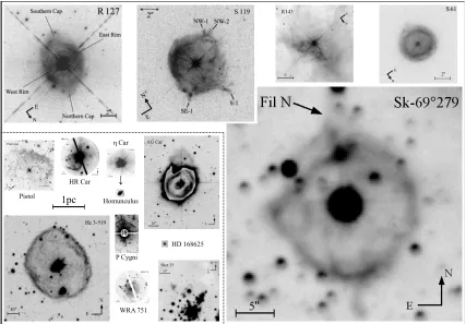
The large stellar winds and great eruptions that are observed in these stars create ejecta

around many of them (Fig. 1.3). The most famous ejection nebula is likely the Homunculus around the massiveηCarinae system, which was observed several times by the Hubble Space Telescope (Davidson & Humphreys 1997) through a Treasury program that examined the spectroscopic and photometric variability for 10 years with excellent spatial resolution.

The LBVs have an interesting geometry surrounding them. The IR excess becomes visible in the optical as this excess is so large. The general schematic is shown in Figure 1.4, where the emitting regions for theR−,H−, andK−bands are shown in comparison to the stellar photosphere and Hα emitting region.

(31)

[image:31.612.93.520.107.404.2]

Figure 1.3 Ejecta surrounding LBVs, drawn to the same physical scale after correction for their individual distances. Diagram reproduced with permission from Weis (2011).

some of the more famous stars in this class.

1.6 BINARIES AND THE LBVS

In massive stellar systems, binaries are common, with more than 75% of O stars in asso-ciations or clusters being multiple systems (Mason et al. 2009). In favorable cases, we can measure their fundamental parameters through analysis of their spectroscopic and photo-metric variability. This is more complicated for LBVs. In the current literature, there are four confirmed binaries in the class, of which two are eclipsing.

(32)

25 Solar Radii

Figure 1.4 The geometry of an LBV wind. The central circle is the stellar photosphere, which is typically has a radius near 75 R⊙. The next circles represent the expected emitting

region sizes for the optical R−band, H−band, and K−band emitting regions, as predicted from spectroscopic models (Hillier & Miller 1998). The largest emitting region shown is for the optically bright emission line Hα. Changes in mass loss rate will make these regions become smaller or larger.

(33)

moderate eccentricity in contrast with most orbits that become circular with time. The small semi-major axis (smaller than the derived radius of HD 5980A during the eruption) allows us a view of the interior of an LBV, as the secondary clears out material, keeping the primary’s radius smaller. This makes this system crucial to modeling of the interiors of LBVs. Indeed the long-term variability (Koenigsberger et al. 2010) shows that the primary star is an LBV, and that even though the primary’s spectrum appears as a W-R star (it is one of the hottest observed LBVs), the secondary has a great influence on the evolution of the system and the primary. The orbital elements and masses are shown in Table 1.2.

Table 1.2: Published Orbital Elements of HD 5980; adapted from Koenigsberger et al. (2010)

Parameter Value Epoch Reference

Porbital 19.2654 d Sterken & Breysacher (1997)

i 88◦

Moffat et al. (1998)

a 127 R⊙ Niemela et al. (1997)

143–157R⊙ Foellmi et al. (2008)

e 0.30±0.16 Foellmi et al. (2008)

MA 50M⊙ Niemela et al. (1997)

58–79 M⊙ Foellmi et al. (2008)

MB 28M⊙ Niemela et al. (1997)

51–67 M⊙ Foellmi et al. (2008)

RA 23–25R⊙ 1978 Perrier et al. (2009)

280 R⊙ 1994 (September) Drissen et al. (2001)

150 R⊙ 1994 (December) Koenigsberger et al. (1998a)

RB 16–17R⊙ Perrier et al. (2009)

LA 3×106L⊙ 1994 (December) Koenigsberger et al. (1998b)

LA 107L⊙ 1994 (September) Drissen et al. (2001)

Tef f,A 21,000 K 1994 (November) Koenigsberger et al. (1996)

Tef f,A 35,500 K 1994 (December) Koenigsberger et al. (1998b)

(34)

and M2 = 3.7+18−2.1.7M⊙. During the primary eclipse, where the smaller star passes in front of

the line of sight of the LBV, we observe an enhanced mass outflow in our line of sight, which is seen from large amounts of blue shifted P Cygni type absorption in all optical wind lines observed. As such, we can expect that mass-loss is larger through the Lagrangian point L1,

which is located between the LBV and the secondary.

The companions in these systems influence the system and the observations of these syetems. Binary interactions are thought to have played a role in the great eruption of η

Carinae (e.g. Smith & Frew 2011). A fundamental question to ask is: Are binary interactions

a driving mechanism for the largest variability of these stars or is it a complication? The

answer can only be found by constraining the multiplicity and orbits of these stars. If binary interactions are a driving force, then we can begin to think about LBV eruption rates in relation to the multiplicity properties.

1.7 OUTLINE OF THIS DISSERTATION

(35)

(36)

THE Hα VARIATIONS OF THE LUMINOUS BLUE VARIABLE P CYGNI: DISCRETE ABSORPTION COMPONENTS AND THE SHORT S

DORADUS PHASE

The results portion of this thesis will begin with a detailed study of the wind of the fa-mous star P Cygni1_{. P Cygni was discovered in the year 1600 when it experienced a great}

eruption and became visible in the constellation Cygnus at the time. It was one of the first variable stars discovered (along with the supernovae of Tycho and Kepler) and is considered a prototypical LBV because of this eruption.

2.1 INTRODUCTION TO P CYGNI

Luminous Blue Variables (LBVs or S Doradus variables) are evolved, massive stars. LBVs are characterized by large mass loss rates and variability on multiple timescales. The two “prototypical” Galactic LBVs are η Carinae and P Cygni, and they probably represent different extremes of mass loss rate within the scheme of LBV evolution (Israelian & de Groot 1999) as these stars likely have very different masses. One of the defining criteria of the LBVs is the observation of a large scale eruption, when the star brightens by several magnitudes. The quiescent times between these eruptions may last centuries. In addition to such rare, giant eruptions, these stars also display lesser photometric and spectroscopic variations on other timescales (e.g. Humphreys & Davidson (1994)). van Genderen (2001) defines the S Doradus (SD-) phase to be the moderate, long-term, brightening and fading phases. There are two types of these phases, short and long, with similar characteristics. The short SD-phase is typically on the order of years (< 10 years), while the longer SD-phase is on a timescale of decades. These phases are thought to originate from changes in the star’s photosphere, and both may have the same physical driving mechanism. These

long-1

(37)

[image:37.612.76.439.109.311.2]

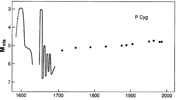
Figure 2.1 A historic light curve of P Cygni, as presented by Humphreys & Davidson (1994)

term variations are observed to differ from cycle to cycle, both in duration and amplitude (Sterken et al. 1997b).

P Cygni (HD 193237, HR 7763, Nova Cyg 1600) remains one of the most fascinating objects in the sky. It was discovered during its first recorded great eruption in 1600 by Willem Janszoon Blaeu, a Dutch chart-maker and mathematician. During this eruption, the star brightened to about 3rd magnitude for about six years, and then it faded from visibility by 1626. It rose again in 1654 to about the same maximal brightness, where it remained for five years. The star faded after this, and although its long-term variability is poorly documented, the star has been slowly brightening to its current magnitude of about 4.8 (Israelian & de Groot 1999). The slow brightening may reflect evolutionary changes (de Groot & Lamers 1992; Lamers & de Groot 1992; Langer et al. 1994). The historical light curve, including the great eruptions of the 17th century, is shown in Figure 2.1.

(38)

a short∼17 day variation similar to theαCygni type variations observed in hot supergiants, a ∼ 100 day “quasi-period” similar to that observed in other LBVs, and a long-term cycle (years) attributed to a short-SD phase (de Groot et al. 2001; Percy et al. 2001).

According to Israelian & de Groot (1999), comprehensive spectral monitoring of P Cygni was started by Luud (1967) and Markova (1993), among others. The first long-term spec-troscopic monitoring campaign of P Cygni was presented in seminal papers by Markova et al. (2001a,b). They found evidence of co-variability of the Hα emission line strength and Johnson U BV photometry, indicating a short-SD phase with a quasi-period of ∼7 years, although their observations did not fully cover two cycles. The variations were attributed to inversely correlated changes in effective temperature and radius, maintaining a nearly constant luminosity. A similar cycle time was found by de Groot et al. (2001), who reported on photometric variations which were consistent with a timescale of 5.5 to 8.5 years.

In addition to the large scale variations in emission strength, Markova (2000) found that there are at least four other kinds of line profile variability in the spectrum of P Cygni. The most striking of these is the long documented appearance of blueward-migrating, absorption sub-features that are called Discrete Absorption Components (DACs: Israelian & de Groot 1999; Markova 2000). These are generally observed in low and intermediate excitation state lines in the optical (Markova 2000) and UV spectrum (Israelian et al. 1996). They are frequently detected in the upper sequence of the H Balmer lines (principal quantum number 9 ≤ n ≤ 15; Markova 2000), but to our knowledge, DACs have not been reported before now for the absorption component of Hα. DACs are often (but not always) narrow (FWHM ≈ 10−15 km s−1_{) and may be unresolved in low-dispersion spectra. The DACs tend to}

appear over a radial velocity range of −90 to −200 km s−1 _{with an acceleration of} ₋₀_._{1 to}

−0.6 km s−1 _d−1_{. A recurrence timescale of} _∼_{200 d is sometimes observed (Markova 1986;}

(39)

1999). The DACs in the spectrum of P Cygni may form in outward moving and dense shells (Lamers et al. (1985); Markova 1986a; Israelian et al. 1996), in spiral-shaped co-rotating interaction regions (CIRs) (Cranmer & Owocki 1996; Markova 2000), or in dense clumps in the wind (L´epine & Moffat 2008).

In this chapter, we present new high resolution Hα spectroscopy, which we combined with previous measurements by Markova et al. (2001) to explore the characteristics of P Cygni’s short SD-phase. We also compare this with archival Johnson V photometry and new observations obtained by AAVSO observers. Section 2.2 describes the observations. In Section 2.3, we present the analysis of long-term variations of the continuum and the Hα

equivalent width. We describe the Hα profile morphology changes and DAC propagations in Section 2.4. The discussion and conclusions are presented in Section 2.5.

2.2 OBSERVATIONS

We obtained 126 new spectroscopic observations of P Cygni using the University of Toledo’s Ritter Observatory 1 m telescope and ´echelle spectrograph (Morrison et al. 1997) between 1999 June 7 and 2007 October 30 (PI N. D. Morrison). These high resolving power (R = 26,000) spectra were reduced by standard techniques with IRAF2_{. Observations collected}

prior to 2007 were taken using the setup described in Morrison et al. (1997). These ob-servations record a 70 ˚A range in the order centered on Hα, and they typically have a signal-to-noise ratio between 50 and 100 per resolution element in the continuum. Observa-tions made during the calendar year 2007 were taken with the same spectrograph, except the camera was a Spectral Instruments 600 Series camera, with a front-illuminated Imager Labs IL-C2004 4100×4096 pixel sensor (15×15 micron pixels). To maintain consistency with the older observations, the camera was operated with 2×2 pixel binning. The newer

observa-2

(40)

tions recorded a larger portion of the order centered on Hα and typically reached a signal to noise ratio between 50 and 100 per resolution element in the continuum. We trimmed these spectra so that the wavelength range was the same as in the older data. The spectra taken after 2002 September have poor wavelength calibration due to problems with the Th-Ar lamp. In order to use these spectra for kinematical measurements, the telluric H2O lines in

the vicinity of Hα were fitted to improve the solution. This worked for most cases, but the errors associated with the telluric re-calibration are roughly ±3 km s−1_{, compared with the}

errors for earlier data of±1 km s−1_.

We collected V-band photometry from three sources. The first was from Markova et al. (2001). This provided concurrent photometry for the Hα data previously published. The second set came from Percy et al. (2001)3_{. These observations also ended at nearly the same}

time as the first data set. Finally, we downloaded the photoelectric photometry in theV-band from the American Association of Variable Star Observers (AAVSO). The AAVSO data are helpful in understanding the long-term trends, and we only used data where measurements of the check and comparison stars differed from expected values by less than 0.05 mag. The errors in the AAVSO measurements are typically around 0.01 mag, comparable to those of Markova et al. (2001) and Percy et al. (2001). The combined set contains 3142 measurements from 1985 to 2009.

2.3 THE LONG-TERM PHOTOMETRIC AND Hα EQUIVALENT WIDTH

VARIABILITY

Markova et al. (2001) found that the Hα line flux, obtained by correcting the observed equivalent widths for the changing continuum, varied in concert with the V-band flux over the period from 1989 to 1999 (see their Fig. 3). Here we extend their work by considering the long-term photometric and Hαvariations through 2007. Figure 2.2 shows the large time

3

(41)

4.6•104 _4.8•104 _5.0•104 _5.2•104 _5.4•104 _5.6•104

HJD - 2,400,000 5.0

4.9 4.8 4.7 4.6

V

(mag)

1985 1990 1995 YEAR2000 2005 2010

Figure 2.2 The V-band variability of P Cygni between 1985 and 2009. The long-term changes are representative of the short SD-phase. We overplotted the fit for the very-long-term brightening of the star with a solid line.

span of available photometry. The light curve over this interval shows rather modest, ±0.1 mag variations, consistent with the star’s classification by van Genderen (2001) as a “weak-active” LBV. It exhibits the kind of variability associated with a short SD-phase, similar to that reported by Markova et al. (2001). The short SD-phase is most evident in the data prior to 2000, when the star experienced two fadings of ≈ 0.1 mag (Markova et al. 2001; Percy et al. 2001). The amplitude of this long-term variability decreased in subsequent years, which indicates that the properties of the short SD-phase change with time. We made a fit of the very-long-term trend and found a brightening rate of ≈ 0.17±0.01 mag century−1

(overplotted in Fig. 2.2). This rate is consistent with the very-long-term trend of 0.15±0.02 mag century−1 _{documented by de Groot & Lamers (1992).}

(42)

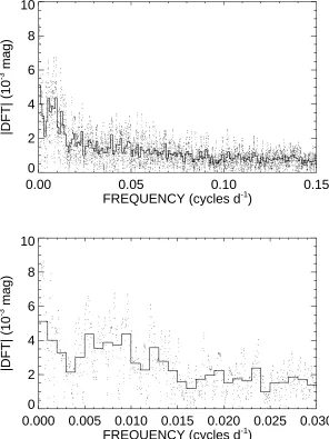
24.5 y V-band photometry with the long-term brightening (Fig. 2.2) removed. There are no individual significant peaks in the periodogram, but there is a general tendency for more power to appear at the longer timescales (lower frequencies). Thus, the longer timescales of the short SD-phase variability tend to dominate the light curve.

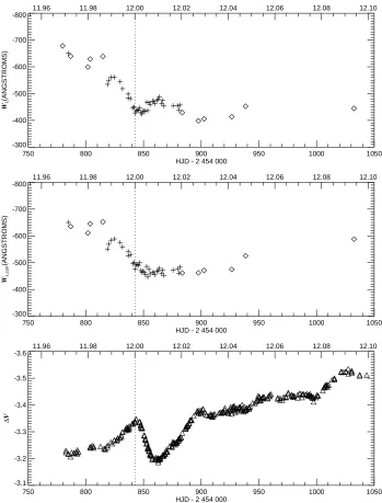
We measured Hα emission strength for both the new and originally reported spectra (Markova et al. 2001) for a total of 158 measurements covering the interval from 1994 to 2007. Equivalent widths of the full Hα profile (including both the blue absorption and large emission component) were measured in the same manner as done by Markova et al. (2001) in order to keep the data sets mutually consistent. The only improvement is that telluric H2O lines in the vicinity of Hα were removed by means of a template fitting procedure

(telluric) in IRAF. This correction resulted in equivalent width increases of less than 2%. This is much smaller than the typical measurement error of 6% (as found by comparing equivalent widths from closely spaced observations, ∆t < 2 d, where the variability of this star is minimal). Since the available wavelength range around Hα does not extend beyond the electron scattering line wings to the actual continuum levels, a multiplicative constant was used to retrieve the full equivalent width of the line. This correction, Wλ(net) = 1.096

Wλ(Ritter), accounts for unseen line wing flux and unmeasured flux lying below our

con-tinuum placement (over an integration range of 6531.5 to 6593.5˚A) and is identical to that adopted by Markova et al. (2001) for the Ritter data. The heliocentric Julian dates and net adjusted equivalent widths are tabulated in columns 1 and 2 of Table B.1.

(43)

0.00 0.05 0.10 0.15

FREQUENCY (cycles d-1)

0 2 4 6 8 10

|DFT| (10

-3 mag)

0.000 0.005 0.010 0.015 0.020 0.025 0.030

FREQUENCY (cycles d-1)

0 2 4 6 8 10

|DFT| (10

[image:43.612.168.464.178.573.2]

-3 mag)

(44)

widths were corrected using the relationship

Wλ(corr) =Wλ(net)10−0.4(V(t)−4.8).

The averagedV magnitudes and flux corrected equivalent widths are given in columns 3 and 4 of Table B.1. If no V magnitude was available within ±20 days, then no correction was applied, which affects 18 of our measurements. These correction factors are usually small (≈4%) and comparable to the photometric scatter within each time window.

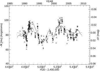
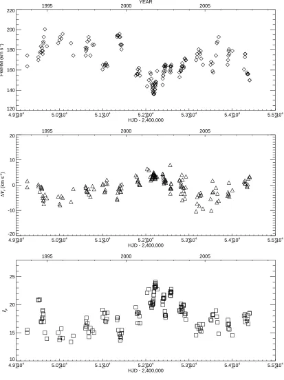
We show the temporal variations in the flux corrected equivalent widths in Figure 2.4. The plot includes earlier measurements from Markova et al. (2001), the new measure-ments from Table B.1, and some additional measuremeasure-ments from 2005 to 2007 from Balan et al. (2010). There are two maxima (occurring around 1992 and 2002) that are separated by ≈ 10 years, which is longer than the reported lengths of the short SD-phase found by Markova et al. (2001), de Groot et al. (2001), or Percy et al. (2001). Furthermore, the rise and fall around the peak in 1992 are steeper than that for the 2002 peak. There is also ample evidence of faster variability within each observing season that appears to be unrelated to the longer term trends.

A visual comparison of the V-band photometry in Figure 2.2 with the flux-corrected Hα

equivalent widths in Figure 2.4 immediately shows some variations in common. We found that the relative flux (from the time interpolated magnitude) is positively correlated with the corrected equivalent width. A linear fit yields a slope of △(F/ < F >)/△(Wλ/ < Wλ >

(45)

4.6•104 _4.8•104 _5.0•104 _5.2•104 _5.4•104 _5.6•104

HJD - 2,400,000 40 60 80 100 120 -W λ [H α ] (Angstroms)

1985 1990 1995 YEAR2000 2005 2010

[image:45.612.151.497.104.355.2]

0.08 0.06 0.04 0.02 0.00 -0.02 -0.04 -0.06 ∆ V (mag)

Figure 2.4 A direct comparison of the smoothed V-band photometry (solid line) and the flux corrected Hα equivalent widths. The photometric light curve is a running average of the V-band flux that was re-scaled and offset to match the equivalent width variations (see text), with the scale of the differential light curve given on the secondary y-axis. A running average of the corrected equivalent width measurements is also overplotted as a dashed line. The equivalent width measurements from Markova et al. (2001) are denoted by diamonds, our new measurements are represented as triangles, and the measurements of Balan et al. (2010) by squares. Uncertainties are comparable to the size of the points.

(46)

this result indicates that the continuum and Hαemission fluxes sample structures in the wind in different ways (probably because of different sites of formation in the outflow). Finally, we note that the correlation also exists between the running averages of the continuum flux and the uncorrected equivalent widthsWλ(net), so the covariations are unrelated to the flux

correction procedure.

2.4 Hα PROFILE MORPHOLOGY VARIABILITY

2.4.1 Emission Component Changes

The large Hα equivalent width variations described in Section 2.3 are accompanied by changes in the morphology of the profile. We present two individual spectra in Figure 2.5 that represent the extrema of the equivalent widths observed (a minimum at HJD 2,450,004, plotted with a dashed-dot line, and a maximum at HJD 2,452,070 plotted with a solid line). It is clear that the profile experiences a change in the peak emission intensity, the line width, the net profile velocity, and the shape of the blue absorption trough. For each of the spectra collected at Ritter Observatory we measured the peak intensity above continuum level, Ip,

which was corrected for the changing continuum level in the same manner as the equivalent width (§3), the FWHM (profile width) of the emission portion of the profile above contin-uum, and a relative radial velocity △Vr, derived by cross-correlating each profile against an

unweighted average of all the spectra obtained at Ritter Observatory. We chose to use a cross-correlation technique because this method is model-free and is most sensitive to the steep emission line wings, resulting in a measure similar to a FWHM bisector velocity. The resulting measurements of FWHM and △Vr are shown for these two profiles in Figure 2.5

with horizontal and vertical lines, respectively.

(47)

Figure 2.5 A comparison of two observed Hα profiles corresponding to extremes of the emission variability (maximum and minimum in corrected equivalent width). The spectrum plotted as a solid line is from HJD 2,452,070, while that shown as a dash-dot line is from HJD 2,450,004. Vertical and horizontal line segments show the velocity offset △Vr and the

FWHM range, respectively.

(for example, HJD 2,452,500; see Fig. 2.4, MJD 5.25·104_{) correspond to profiles with the}

largest peak intensity and smallest FWHM. We also see a small radial velocity shift that is correlated with the long-term variations. The profile had the largest (most positive) velocity when the line flux at the position of the emission peak was strongest, which was also when the profile showed the smallest FWHM (Fig. 2.6). This is likely due to changes in the P Cygni absorption component. When the profile has the most emission, the blue absorption portion appears to shift to a more positive velocity and removes more of the blue side of the emission peak (see Fig. 2.5), and thus, the net radial velocity tends toward a larger (more positive) value at those times. We find that the measurement errors for△Vr and the FWHM

(48)

yield net errors of approximately ±1.5 km s−1 _{for most of the data, and} _±₃_._{2 km s}−1 _for

data taken after 2002 September. The errors for Ip are on the order of 3−5%.

Kashi (2010) has suggested P Cygni is a binary system with a fainter B-type companion and that small long-term radial velocity variations due to reflex motion might be observed in extended high resolution spectroscopic observations. This cannot be the explanation for the △Vr changes we observe, since the Hα emission is formed over a volume that is much larger

in radius than the predicted semimajor axis of the putative orbit of the P Cygni primary star. Wind gas leaving the star at any instant would have a Keplerian orbital component that decreases with distance from the center of mass. As the gas packet moves out to the radius where Hα becomes optically thin and emits the photons we observe (at≈ 10R⋆ and

larger; see below), the radial outflow component will increase by radiative driving while the orbital motion component will drop with distance to conserve angular momentum. Thus, at the large distance of line formation, the gas motion will be almost completely radial. If the putative companion is to be found from radial velocity variations of this star, then detailed analyses of photospheric or wind lines formed very close to the star will need to be analyzed. Further, these radial velocity variations are not strictly periodic, and cannot be considered orbital motion. Lastly, given the method of measuring these velocities, the measured radial velocity is at least partially due to morphological changes in the Hα line profile.

2.4.2 Blue Absorption Changes

(49)

4.9•104 5.0•104 5.1•104 5.2•104 5.3•104 5.4•104 5.5•104

HJD - 2,400,000 120 140 160 180 200 220

FWHM (km s

-1)

1995 2000 YEAR 2005

4.9•104 5.0•104 5.1•104 5.2•104 5.3•104 5.4•104 5.5•104

HJD - 2,400,000 -20 -10 0 10 20 ∆ Vr (km s -1)

1995 2000 2005

4.9•104 5.0•104 5.1•104 5.2•104 5.3•104 5.4•104 5.5•104

HJD - 2,400,000 10

15 20 25

Ip

[image:49.612.107.520.106.659.2]

1995 2000 2005

Figure 2.6 The long-term variability of the FWHM (top panel), the relative radial velocity △Vr (middle panel), and flux corrected peak intensity Ip (bottom panel) of the emission

peak of the Hα profile. The long timescales of variability are similar to those seen in the

(50)

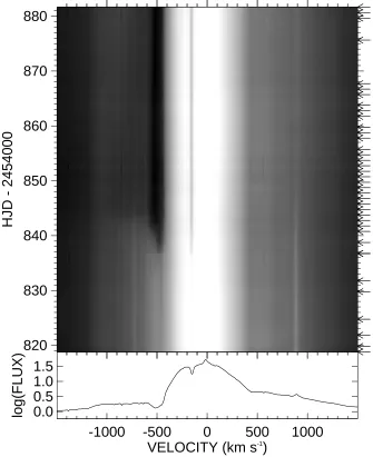
intensity and then constructed the average of all the intensities falling between the 90th and 95th percentiles at that wavelength step. This removed any spurious peaks caused by cosmic rays from contaminating the minimum absorption average. We then divided each of the spectra by this reference spectrum to form a matrix of quotient spectra. Since we are interested in the variability of the central absorption, and not that of the far wings, and because the line wings never reach the continuum in the region recorded, the quotient spectra had a depressed continuum. We then re-normalized these to a unit continuum (outside of the velocity region ±500 km s−1_{). These spectra are illustrated in a gray-scale dynamical}

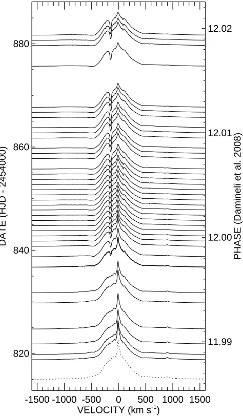
spectrum in Figure 2.7. In this figure, we present each quotient spectrum as a function of radial velocity and time with a gray-scale intensity between the minimum value (black; 0.14 in the quotient) and maximum value (white; 1.75 in the quotient) based upon a linear time interpolation between the nearest observations (indicated by arrows). The low absorption reference spectrum is displayed for comparison in a panel below the gray-scale image. For simplicity, these quotient spectra were not corrected for the variable continuum flux since we are interested in both emission and absorption changes.

We need to bear in mind that the low absorption spectrum was formed by different sub-samples at each wavelength point, and this has important consequences for the appearance of the dynamical spectrum. For example, inspection of Figure 2.5 shows that blue absorp-tion core can extend to high negative velocities (dash-dot line) while at other times the blue absorption is limited to moderate velocities (solid line). Thus, the construction of the low absorption spectrum will be dominated by the latter examples in the vicinity of the blue absorption edge, and in our collection of Hα spectra, the more extended blue absorption occurred much more frequently. Consequently, the quotient spectra in Figure 2.7 appear to be dominated by a blue absorption feature, near −220 km s−1_{, except near HJD 2,452,500}

(MJD 5.25·104_{) when the blue edge moved to a more positive velocity. This feature is due}

(51)

absorp--200 0 200

VELOCITY (km s-1

) 0

10 20

0

INTENSITY

5.0•104

5.1•104

5.2•104

5.3•104

5.4•104

HJD - 2,400,000

(52)

tion spectrum. We made this selection for our template so that the subfeatures appear in absorption most of the time.

We also see evidence in Figure 2.7 of several blueward moving, absorption features (in the velocity range between −100 and −200 km s−1_{) that appear morphologically similar}

to the Discrete Absorption Components (DACs) observed previously in other spectral lines (Israelian & de Groot 1999; Markova 1986a, 2000). Figure 2.8 is a montage of a subset of the quotient spectra. It shows how the DAC (center) moved progressively blueward over this time span (≈ 800 d). There are times where the regions between successive DACs appear bright in the dynamical spectrum, which correspond to those cases (usually sparsely sampled in time) where the flux was higher than the mean in the 90% to 95% part of the flux distribution that defined the minimum absorption spectrum. Finally, we see in the gray-scale image of Figure 2.7 the long-term variations in peak intensity (Ip) and wing extension

(FWHM) that are associated with the short SD-phase, equivalent width variations (Fig. 2.6). We measured the variability of the quotient spectra by calculating the standard deviation at each pixel of velocity space. This standard deviation spectrum is shown in Figure 2.9. There is a broad feature centered at rest velocity which is associated with the varying peak height of the profile. Another feature is present at ∼ +150 km s−1_{, which could be caused}

by either the variations in the profile width (FWHM) or red emission wing variability from traveling bumps (Markova 2000). The largest two features are from the DACs (seen as a broad peak around −140 km s−1_{) and from the variations present near the blue edge of the}

absorption core (visible as a peak centered at−220 km s−1_).

(53)

-300

-200

-100

0 V

_r

(km s

-1

)

0

2

4

6

8

10 NORMALIZED INTENSITY

50614.794

51445.630

Figure 2.8 A series of quotient spectra offset according to the time of observation (HJD − 2,400,000 indicated for the first and last spectrum in this sequence). The DAC present migrated from approximately −125 km s−1 _to ₋_{160 km s}−1 _{over this interval. The dotted}

(54)

-400 -200 0 200 400

Vr (km s

-1

) 0.0

0.1 0.2 0.3

SIGMA

Figure 2.9 The pixel-by-pixel standard deviation of the quotient spectra (solid line). We also show the low absorption reference profile (dotted line; re-scaled to this range) to highlight those parts of the profile where the largest relative variations are occurring: near the terminal velocity blue edge (near −220 km s −1_{), over the range traversed by the DACs (centered}

near≈ −150 km s−1_{), near the emission peak (0 km s} −1_{), and in the emission wings (}_±₁₅₀

km s −1_{). The standard deviation of the quotient is larger in the absorption core because}

the low absorption profile is close to zero there.

often poorly constrained because absorption may extend blueward with a shallow slope (see Fig. 2.5). Thus, we decided instead to document the kinematical changes near the blue edge by measuring the position of the absorption core flux minimum, Vr(min), which is normally

found near−210 km s−1 _{where the slope of the profile changes sign abruptly. We determined}

this position by finding the zero crossing in the numerical derivative of a smoothed version of the spectrum. The S/N ratio was sufficient in all our spectra that the zero of the derivation was always well-defined. This estimate of the minimum flux velocity Vr(min) is given in

column 8 of Table B.1, and the errors in Vr(min) are comparable to the errors associated

(55)

wind speed at a location in the wind where Hα ceases to be optically thick.

It is difficult to measure the radial velocities of the DACs because their morphologies vary and because the absorption may consist of multiple components. We decided to measure a centroid for the DACs wherever possible by means of the relationship

Vr(DAC) =

Rv2

v1 vr(1−Q(vr))dvr

Rv2

v1 (1−Q(vr)) dvr

whereQrepresents the quotient spectrum andvr is the radial velocity. We adopted a velocity

range of v1 =−200 km s−1 and v2 =−100 km s−1 based upon the strongest regions of the

standard deviation spectrum plotted in Figure 2.9. Typical errors in these measurements (from the scatter in densely sampled regions of the time series) are±3 km s−1_{. This approach}

worked for most of the spectra, but some low contrast features were not measured correctly, and are omitted from Table B.1 and our analysis. During some epochs, there were multiple DACs present, so Vr(DAC) represents a weighted average of multiple components. The

DAC radial velocities Vr(DAC) are given in column 9 of Table B.1. Column 10 lists a

relative equivalent width for the DAC measured by a direct numerical integration of Q(vr)

between v1 and v2. The typical errors associated with these equivalent width measurements

are on the order of 5%, which is similar to the errors associated with the equivalent widths of the profile (§3).

(56)

mea-4.9•104 _5.0•104 _5.1•104 _5.2•104 _5.3•104 _5.4•104 _5.5•104

HJD - 2,400,000 -100

-120 -140 -160 -180 -200 -220

Vr

(km s

-1 )

1995 2000YEAR 2005

Figure 2.10 The temporal variations of the measured velocities of the DACs, Vr(DAC)

(plus signs), and the minimum flux wind velocities, Vr(min) (diamonds). The dashed line

represents the acceleration fit to the DAC progression near HJD 2,451,000, and the dotted lines represent the same fit translated by intervals of 1700 days, which we derived as a possible recurrence time.

sured the acceleration to be−0.047±0.002 km s−1 _d−1_{. For comparison, the observed DACs}

in the spectrum of a normal hot supergiant of similar spectral type,ǫOri (HD 37128; B0 Ia), have an acceleration of−500 km s−1 _d−1 _{(Prinja et al. 2002).}

(57)

velocity centroid we measured represents a blend of these components. Neither of these two DACs occurred at the expected recurrence time in the 1700 d cycle.

Our work represents the first detection of DACs in the blue absorption trough of Hα, and their properties differ from those observed in other spectral lines (Israelian et al. 1996; Markova 1986, 2000). For example, the recurrence timescale of 1700 d is much larger than the 200 d interval found in earlier work, and the acceleration measured is about a factor of 10 smaller than measured by others for ultraviolet lines of P Cygni. It is suspected that these differences are due to the large optical depth of the Hα line compared to that of other lines where DACs have been investigated. This will mean that the radius of optical depth unity is larger for Hα (Najarro et al. 1997), and consequently any wind structures formed at smaller radii will have no affect on the Hα line formation. It could be suspected that observations of other, less optically thick lines are more sensitive to the detection of DACs formed at smaller radii in the wind of P Cygni where more and faster accelerating structures may exist.

2.5 DISCUSSION

(58)

that the mass loss rate is high (≈ 2×10−5 _M

⊙ y−1 including wind clumping effects) and

wind terminal velocity is low (v∞ = 185 km s−1). Najarro et al. (1997) derive a systemic

velocity of γ = −29 km s−1_{, and thus our minimum measurement of} _V

min = −215 km s−1

is consistent with their estimate of γ −v∞ = −214 km s−1 as this velocity measurement

is related to v∞. They estimate that the continuum forming radius is 76R⊙, which for

a distance of 1.8 kpc implies an angular diameter of θ = 0.39 mas. On the other hand, Najarro et al. (1997) predict that the emitting size of Hα will be much larger because of its greater optical depth. For example, their models show that there is a local maximum in the wind temperature distribution (presumably where the recombination processes that form Hα peak) nearr/R⋆ = 11 (see their Fig. 2.6b). The corresponding angular size for Hα

of ≈4 mas agrees well with the range of 3−7 mas from Hα interferometry by Balan et al. (2010). Thus, we need to keep in mind that the Hα variations reflect changes over a much larger spatial scale in the wind than those observed in the V-band flux.

Variations in the Hα emission equivalent width are related to changes in both the mass loss rate and the wind velocity. In a very simplified approach, it can be assumed that most of the Hα flux originates in the optically thick region projected on the sky,

f =πr_τ2F(T)

wererτ is the boundary separating the optically thick and thin regimes,F(T) is the

monochro-matic surface flux, and T is the wind temperature atrτ (Najarro et al. 1997). If we assume

that the wind is approximately isothermal at this physical location (a reasonable choice: see Fig. 5b in Najarro et al. 1997), then the emission flux variations are due to changes in the projected size of the optically thick region,

(59)

Thus, it is expected that the relative variations in angular size will be only half as large as the emission equivalent width variations, which is probably consistent with the lack of measurable size changes in the Hα interferometric measurements (Balan et al. 2010).

The Hα optical depth is dependent on the electron density squared since the emission is a recombination process. Thus, we expect that the optical depth unity boundary rτ will

always be defined by the location in the wind with a specific characteristic density, ρτ. We

assume that ρτ has an approximately constant value so that the effective rτ boundary will

vary as fluctuations in the wind mass loss rate and velocity define the radius where the density reaches ρτ. According to the mass continuity equation, rτ is related to this density

by

r2_τ = M˙

4πρτv

where ˙M is the mass loss rate and v is the wind velocity at the radial distance rτ. We can

differentiate the mass continuity equation to express the radius variation in terms of the changes in ˙M and v,

2rτ△rτ =

1 4πρτ

△[ ˙M /v],

which we divide by r2

τ to obtain

2△rτ

rτ