https://doi.org/10.5194/hess-22-1193-2018 © Author(s) 2018. This work is distributed under the Creative Commons Attribution 3.0 License.
Parametric soil water retention models: a critical evaluation of
expressions for the full moisture range
Raneem Madi1, Gerrit Huibert de Rooij1, Henrike Mielenz2, and Juliane Mai3,a
1Dept. Soil System Science, Helmholtz Centre for Environmental Research – UFZ, Halle, Germany 2Institute for Crop and Soil Science, Julius Kühn-Institut – JKI, Braunschweig, Germany
3Dept. Computational Hydrosystems, Helmholtz Centre for Environmental Research – UFZ, Leipzig, Germany acurrently at: Dept. Civil & Environmental Engineering, Univ. of Waterloo, Waterloo, Canada
Correspondence:Gerrit Huibert de Rooij ([email protected]) Received: 12 April 2016 – Discussion started: 25 April 2016
Revised: 4 January 2018 – Accepted: 8 January 2018 – Published: 12 February 2018
Abstract.Few parametric expressions for the soil water re-tention curve are suitable for dry conditions. Furthermore, expressions for the soil hydraulic conductivity curves asso-ciated with parametric retention functions can behave unre-alistically near saturation. We developed a general criterion for water retention parameterizations that ensures physically plausible conductivity curves. Only 3 of the 18 tested pa-rameterizations met this criterion without restrictions on the parameters of a popular conductivity curve parameterization. A fourth required one parameter to be fixed.
We estimated parameters by shuffled complex evolution (SCE) with the objective function tailored to various obser-vation methods used to obtain retention curve data. We fitted the four parameterizations with physically plausible conduc-tivities as well as the most widely used parameterization. The performance of the resulting 12 combinations of retention and conductivity curves was assessed in a numerical study with 751 days of semiarid atmospheric forcing applied to unvegetated, uniform, 1 m freely draining columns for four textures.
Choosing different parameterizations had a minor effect on evaporation, but cumulative bottom fluxes varied by up to an order of magnitude between them. This highlights the need for a careful selection of the soil hydraulic parameter-ization that ideally does not only rely on goodness of fit to static soil water retention data but also on hydraulic conduc-tivity measurements.
Parameter fits for 21 soils showed that extrapolations into the dry range of the retention curve often became physi-cally more realistic when the parameterization had a
loga-rithmic dry branch, particularly in fine-textured soils where high residual water contents would otherwise be fitted.
1 Introduction
The pore architecture of the soil influences its hydraulic behavior, typically described by two curves: the relation-ship between the amount of water present in the soil pores and the matric potential (termed soil water characteristic or soil water retention curve), and the relationship between the hydraulic conductivity and either matric potential or water content (the soil hydraulic conductivity curve). Numerical solvers of Richards’ equation for water flow in unsaturated soils require these curves as descriptors of the soil in which the movement of water should be calculated. Many paramet-ric expressions for the retention curve and fewer for the hy-draulic conductivity have been developed for that purpose (see the Supplement, Leij et al., 1997; Cornelis et al., 2005; Durner and Flühler, 2005; Khlosi et al., 2008; Assouline and Or, 2013).
(Klute, 1986, pp. 644–647) typically gave a more smooth shape around the matric potential where the soil started to desaturate as an artefact of the sample height, as was later demonstrated by Liu and Dane (1995). This led to the in-troduction of parameterizations that yielded a continuously differentiable curve.
The interest in the dry end of the retention curve was trig-gered by an increased interest in water scarcity issues (e.g., Scanlon et al., 2006; UN-Water, FAO, 2007; UNDP, 2006). For groundwater recharge under deep vadose zones, the dry end of the soil water retention curve affects both slow liquid water movement in film and corner flow (Tuller and Or, 2001; Lebeau and Konrad, 2010) and vapor phase transport (Barnes and Turner, 1998; de Vries and Simmers, 2002). The earlier parameterizations had an asymptote at a small (or at zero) water content. This often gave poor fits in the dry end, and several parameterizations emerged in which the dry branch was represented by a logarithmic function that reached zero water content at some point.
A nonparametric approach was advocated by Iden and Durner (2008). They estimated nodal values of volumetric water content from evaporation experiments and derived a smooth retention curve by cubic Hermite interpolation. They extrapolated the retention function to the dry range and com-puted a coupled conductivity function based on the Mualem model.
Liu and Dane (1995) were the first to point out that the smoothness of observed curves around the air-entry value could be an artefact related to experimental conditions. Fur-thermore, it became apparent that a particular parameteri-zation that gave a differentiable curve led to unrealistically large increases of the soil hydraulic conductivity near sat-uration (Durner, 1994; Vogel et al., 2001). This was even-tually linked to the nonzero slope at saturation (Ippisch et al., 2006), implying the existence of unphysically large pores with air-entry values up to zero. This led to the reintroduction of a discrete air-entry value.
Most of the parameterizations are empirical, curve-fitting equations (Kosugi et al., 2002). One exception is the very dry range, where measurement techniques are often not so reliable (e.g., Campbell and Shiozawa, 1992) and were not always employed. The proportionality of the water content in this range to the logarithm of the absolute value of the matric potential that has frequently been invoked conforms to the adsorption theory of Bradley (1936), which considers adsorbed molecules to build up in a film consisting of layers, with the net force of electrical attraction diminishing with every layer (Rossi and Nimmo, 1994).
The empirical power-law relationship between water content and matric potential introduced by Brooks and Corey (1964) was later given a theoretical foundation by Tyler and Wheatcraft (1990), who showed that the exponent was related to the fractal dimension of the Sierpenski carpet used to model the hierarchy of pore sizes occurring in the soil. The sigmoid shape of the Kosugi’s (1996, 1999)
reten-tion curve was derived rigorously from an assumed lognor-mal distribution of effective pore sizes, making this the only parameterization discussed in this paper developed from a theoretical analysis.
Some soils have different types of pore spaces: one type appears between individual grains. Its architecture is deter-mined by soil texture, and by the geometry of the packing of the individual grains. The second type appears on a larger scale: the soil may consist of aggregates (e.g., Coppola, 2000, and references therein), and the pore space between these ag-gregates is very different from those between the grains. Bio-pores formed by roots that have since decayed, soil fauna, etc. can also create a separate type of pore space. In shrink-ing soils, a network of cracks may form. The volume and ar-chitecture of these pore spaces are essentially independent of the soil texture (Durner, 1994), even though a certain texture may be required for these pores to form. In soils with such distinct pore spaces, the derivative of the soil water retention curve may have more than a single peak, and for this rea-son multimodal retention curves have been proposed, e.g., by Durner (1994) and Coppola (2000). Most of the parametric expressions for the soil water retention curve are unimodal though. Durner (1994) circumvented this by constructing a multimodal retention curve by summing up several sigmoidal curves of van Genuchten (1980) but with different param-eter values. He presented excellent fits of bimodal reten-tion funcreten-tions at the price of adding three or four parame-ters, depending on the chosen parameterization. Priesack and Durner (2006) derived the corresponding expression of the hydraulic conductivity function. Romano et al. (2011) devel-oped a bimodal model based on Kosugi’s (1994) curve and derived the associated hydraulic conductivity function. Cop-pola (2000) used a single-parameter expression for the intra-aggregate pore system superimposed on a five-parameter ex-pression for the inter-aggregate pores, thereby reducing the number of fitting parameters and the degree of correlation among these. The primary focus of this paper is on unimodal functions, but we briefly discuss three multimodal models as well.
The wealth of parameterizations for the soil water reten-tion curve calls for a robust fitting method applicable to vari-ous parameterizations and capable of handling data with dif-ferent data errors. These errors arise from the various mea-surement techniques used to acquire data over the full wa-ter content range. Paramewa-ter fitting codes are available (e.g., Schindler et al., 2015), but they do not fit the parameteriza-tions focusing on the dry end. The first objective of this paper is to introduce a parameter fitting procedure that involves an objective function that accounts for varying errors, embedded in a shell that allows a wide spectrum of retention function parameterizations to be fitted.
con-ductivity model only. Iden et al. (2015) approached the same problem but only examined the conductivity curve. They too focused on the van Genuchten–Mualem configuration only. The analysis of Ippisch et al. (2006) could well have rami-fications for other parameterizations. A second objective of this paper is therefore the development of a more general analysis based on Ippisch et al. (2006) and its application to other parameterizations of the retention and conductivity curves.
Several hydraulic conductivity parameterizations that re-lied only on observations of soil water retention data have been developed (see the reviews by Mualem, 1992 and As-souline and Or, 2013). Many of these consider the soil layer or sample for which the conductivity is sought as a slab of which the pore architecture is represented by a bundle of cylindrical tubes with a given probability den-sity function (PDF) of their radii. This slab connects to an-other slab with a different pore radius PDF. By making dif-ferent assumptions regarding the nature of the tubes and their connectivity, different expressions for the unsaturated hydraulic conductivity can be found (Mualem and Dagan, 1978). Raats (1992) distinguished five steps in this process: (1) specify the effective areas occupied by connected pairs of pores of different radii that reflect the nature of the cor-relation between the connected pore sizes; (2) account for tortuosity in one of various ways; (3) define the effective pore radius as a function of both radii of the connected pairs of pores; (4) convert the pore radius to a matric potential at which the pore fills or empties; and (5) use the soil water re-tention curve to convert from a dependence upon the matric potential to a dependence upon the water content. Only step 5 constitutes a direct effect of the choice of the retention curve parameterization on the conductivity curve. Choices made in steps 1–3 result in different conductivity curves associated with any particular retention curve parameterization.
These conductivity parameterizations give the hydraulic conductivity as a function of matric potential or water con-tent relative to the value at saturation. They therefore require a value for the saturated hydraulic conductivity, either inde-pendently measured or estimated from soil properties. As-souline and Or (2013) review numerous expressions for the saturated hydraulic conductivity. Interestingly, approaches have emerged to estimate the saturated hydraulic conductiv-ity from the retention curve parameters (Nasta et al., 2013; Pollacco et al., 2013, 2017).
The functions based on the pore bundle approach dis-cussed by Mualem and Dagan (1978), Mualem (1992), and Raats (1992) that have found widespread application in nu-merical models can be captured by Kosugi’s (1999) gener-alized model. In this paper, we limit ourselves to three pa-rameterizations as special cases of Kosugi’s general model, and discuss them in more detail in Sect. 2. In doing so, we add to the existing body of comparative studies of paramet-ric retention curves by explicitly including the associated hydraulic conductivity curves according to these
conductiv-ity models. Papers introducing new parameterizations of the soil water retention curve as well as reviews of such pa-rameterizations typically show the quality of the fit to soil water retention data (e.g., van Genuchten, 1980; Rossi and Nimmo, 1994; Cornelis et al., 2005; Khlosi et al., 2008). The role of these parameterizations is to be used in solutions of Richards’ equation, usually in the form of a numerical model. Their performance can therefore be assessed through the wa-ter content and wawa-ter fluxes in the soil calculated by a numer-ical Richards solver. This is not often done, one exception be-ing the field-scale study by Coppola et al. (2009) comparbe-ing unimodal and bimodal retention curves and the associated conductivity curves in a stochastic framework on the field scale, for a 10-day, wet period. A third objective therefore is to carry out a numerical modeling exercise to examine the differences in soil water fluxes calculated on the basis of var-ious parameterizations by the same model for the same sce-nario. By doing so, the inclusion of the conductivity curves in the comparison is taken to its logical conclusion by carry-ing out simulations for all possible combinations of retention and conductivity models.
Should the differences in the fluxes be small, the choice of the parameterizations can be based on convenience. If they are significant, even if the fits to the data are fairly similar, this points to a need for a more thorough selection process to determine the most suitable parameterization.
2 Theory
2.1 Hydraulic conductivity models and their behavior near saturation
Numerous functions have been proposed to describe the soil water retention curve, several of them reviewed below. Fewer functions exist to describe the soil hydraulic conductivity curve. When these rely on the retention parameters, one can use the retention curve to predict the conductivity curve. However, when both retention and conductivity data exist, a single set of parameters does not always fit both curves well, even if both sets of data are used in the fitting process. It may therefore be prudent to attempt to find a retention– conductivity pair of curves that shares a number of param-eters that could be fitted on retention data only and has ad-ditional parameters that only occur in the expression for the hydraulic conductivity.
Ko-sugi (1999) is as follows:
K(Se)=KsSeτ
Se R 0
|h|−κ(x)dx
1 R 0
|h|−κ(x)dx
γ , (1)
where the subscriptsdenotes the value at saturation,x is an integration variable, andγ,κ, andτ are dimensionless shape parameters. The degree of saturationSeis defined as follows:
Se(h)=
θ (h)−θr θs−θr
, (2)
where the subscriptrdenotes the irreducible value (≥0). Af-ter a change of variables this gives (Ippisch et al., 2006)
K(h)=K(h(Se))=
KsSeτ
h(Se ) R −∞
|h|−κdS
dhdh hae
R
−∞
|h|−κdS
dhdh
γ
, h≤hae
Ks, h≥hae,
(3)
wherehae[L] is the air-entry value of the soil andSdenotes the degree of saturation moving between 0 and the actual value Se. Note that the value of S(h) and dS /dh are
di-rectly related to the soil water retention curveθ (h)through Eq. (2). Specific models can be found by fixing the parame-ters: Burdine’s (1953) model is obtained with γ=1,κ=2, and τ=2, the popular model of Mualem (1976) results when γ=2, κ=1, andτ=0.5, and the model of Alexan-der and Skaggs (1986) requires γ=κ=τ=1. Assouline and Or (2013) give parameter values for additional conduc-tivity models. When any of these models are used, the soil water retention parameters can be used to predict the con-ductivity curve if no concon-ductivity data are available and the saturated hydraulic conductivity can be estimated indepen-dently (see Jarvis et al., 2002, and references therein). Note that positive values ofκensure that large pores (emptying at smaller values of|h|)contribute more to the overall hydraulic conductivity than small pores, which is a physically sound condition. Parameterγ should be positive as well. Negative values would lead to a switch of the numerator and denom-inator (which scales the numerator by its maximum value) in Eq. (1), which is illogical. Peters (2014) required that the conductivity curve monotonically decreases as the soil dries out and derived a minimal value of −2 forτ from that re-quirement. Indeed, negative values of this parameter have been reported (e.g., Schaap and Leij, 2000), even though the three predictive models mentioned above all have positive values ofτ.
Driven by the occasionally unrealistic shape of Mualem’s (1976) hydraulic conductivity curve near saturation, Ippisch et al. (2006) rigorously analyzed the version of Eq. (3) specific to Mualem’s (1976) model. They concluded that the integrand must approach zero near saturation in order to prevent unrealistically large virtual
pores dominating the hydraulic conductivity of very wet soils, a point raised earlier by Durner (1994). We generalize their criterion for prohibiting excessively larger pores from dominating the conductivity near saturation for arbitrary parameter values (after converting dS /dhto dθ /dh) by
lim
h→0
|h|−κdθ
dh
=0. (4)
This condition is automatically met by retention curves with nonzero air-entry values, but restricts the permissible value of κif the retention curve has nonzero derivatives at saturation and couples it to this derivative.
Iden et al. (2015) argued that limiting the maximum pore size of the pore-bundle models that gave rise to models of the type of Eq. (1) eliminated the large pores that caused the excessively rapid rise of the hydraulic conductivity near satu-ration. By only modifying the conductivity function without changing the water retention function, a discrepancy emerges between the retention curve (which reflects the presence of unphysically large pores) and the conductivity curve (which does not). Retention curves with a distinct air-entry value maintain the desired consistency, at the price of having non-continuous derivatives. Computational tests by Ippsisch et al. (2006) suggest that state-of-the-art numerical solvers of Richards’ equation are capable of handling this.
2.1.1 Critical evaluation of unimodal parametric functions of the soil water retention curve
The Supplement reviews 18 parameterizations of the soil wa-ter retention curve. Their derivatives are presented and used to verify the physical plausibility of the hydraulic conductiv-ity near saturation according to Eq. (4). In this section only those equations that satisfy the criterion in Eq. (4) are pre-sented, together with the associated hydraulic conductivity functions. For comparison, the most widely used parameter-ization is also included here. To facilitate cross-referencing between the Supplement and the main text, the equations lifted from the Supplement into the main text have the same number in the main text as in the Supplement.
The water retention function of Brooks and Corey (1964) is
θ (h)= (
θr+(θs−θr)
h hae
−λ
, h≤hae θs, h > hae,
(S1a) whereλis a dimensionless fitting parameter. This equation is referred to as BCO below. The analytical expression for the generalizedK(h)function (Eq. 3) for the water retention function of Brooks and Corey (1964) is
K(h)= Ks
h(Se)
hae −λτ
λ(θs−θr)|hae|λ
κ+λ+2 |h|
−κ−λ
h −∞ hλ(θ
s−θr)|hae|λ
κ+λ+2 |h|
−κ−λihae
−∞ γ
=Ks
hae
h
λ(γ+τ )+γ κ
, h≤hae
Ks, h > hae.
Van Genuchten’s (1980) formulation is continuously dif-ferentiable:
θ (h)=θr+(θs−θr) 1+ |αh|n −m
, h≤0, (S4a)
where α [L−1], n, and m are shape parameters. Often m is set equal to 1−1/n. This equation is denoted by VGN below. The hydraulic conductivity only exhibits acceptable behavior near saturation if κ <n−1. For many fine and/or poorly sorted soil textures,nranges between 1 and 2. There-fore, this restriction even excludes Mualem’s (1976) con-ductivity model whenn< 2. For this reason we refrain from formulating analytical conductivity equations, even though van Genuchten (1980) presented such expressions for Bur-dine’s (1953) and Mualem’s (1976) models. Because of its popularity we will include it in the further evaluation any-way.
Ippisch et al. (2006) proposed to introduce an air-entry value and scale the unsaturated portion of VGN by its value at the water-entry value:
θ (h)= (
θr+(θs−θr)
1+|αh|n 1+|αhae|n
−m
, h < hae
θs, h≥hae,
(S7a)
This equation is labeled VGA below. With the common restriction of m=1−1/n, an expression can be found for κ=1 that is slightly more general than Eq. (11) in Ippisch et al. (2006): K(h)= Ks
θ−θ r θs−θr
τ
1−
1− 1
B(h) n
n−1
1−1−1
C n
n−1
γ
=Ks
B(h)
C
τ1n−1
1−
1−B(h)1
n n−1
1−1−1
C n
n−1
γ
,
h < hae
Ks, h≥hae,
(S7c)
where
B(h)=1+ |αh|n, (S7d)
C=1+ |αhae|n. (S7e)
This equation can be used to define conductivity mod-els according to Mualem (1976) and Alexander and Sk-aggs (1986), which both require thatκ=1.
Rossi and Nimmo (1994) preferred a logarithmic func-tion over the Brooks–Corey power law at the dry end to better represent the adsorption processes that dominate wa-ter retention in dry soils, as opposed to capillary processes in wetter soils. They also implemented a parabolic shape at the wet end as proposed by Hutson and Cass (1987). Rossi and Nimmo (1994) presented two retention models, but only one (the junction model) permitted an analytical expression of the unsaturated hydraulic conductivity. Here, we modified the junction model by removing the parabolic expression for
the wet end of the retention curve in favor of the discontinu-ous derivative at the air-entry value:
θ (h)=
0, h≤hd
θsβln
hd h
, hd< h≤hj θs
hae h
λ
, hj< h≤hae θs, h > hae
, (S9a)
which is denoted as RNA below.
Rossi and Nimmo (1994) required the power law and logarithmic branches as well as their first derivatives to be equal at the junction point (θj,hj). Withhdfixed (Rossi and Nimmo found a value of−105m for six out of seven soils and−5×10⁵m for the seventh), these constraints allow two of the five remaining free parameters to be expressed in terms of the other three. Some manipulation leads to the following expressions:
λ= 1
ln|hd| −ln hj
, (S9c)
β=λ
hae hj
λ
. (S9d)
This gives the fitting parametershae,hj, andθs. The asso-ciated conductivity model is
K(h)=
0, h≤hd
KsSτe
h
−θsβκ |h|−κih
hd
h
−θsκβ|h|−κihj
hd
−hθsλ
λ+κ|hae|λ|h|
−(λ+κ)ihae hj γ
=Ks h βln h d h iτ E(h) E(hj)+F
hj
−λ−κ
−|hae|−λ−κ γ ,
hd< h≤hj
KsSτe h −θsβ
κ |h|
−κihj hd−
hθ
sλ λ+κ|hae|λ|h|
−(λ+κ)ih hj
h
−θsκβ|h|−κihj
hd
−hθsλ
λ+κ|hae|λ|h|
−(λ+κ)ihae hj γ
=Ks hae h λτ
E(hj)+F
hj
−λ−κ
−|h|−λ−κ
E(hj)+F
hj
−λ−κ
−|hae|−λ−κ γ ,
hj< h≤hae
Ks, h > hae,
(S9e)
where E(h)=β
κ |hd|
−κ− |h|−κ
, (S9f)
F = λ
λ+κ|hae|
λ. (S9g)
Fayer and Simmons (1995) used the approach of Camp-bell and Shiozawa (1992) to have separate terms for adsorbed and capillary-bound water. If the capillary binding is repre-sented by a Brooks–Corey-type function, the retention model becomes
θ (h)=
0, h≤hd
θa
1− ln|h| ln|hd|
+
h θs−θa
1− ln|h|
ln|hd| i h
ae
h
λ , hd< h < hae
θs, h≥hae.
This expression is denoted FSB below. Note that this model is valid ifhaedoes not exceed−1 cm. This condition will usually be met, unless the soil texture is very coarse. The corresponding conductivity model is
K(h) =
0, h≤hd
KsSτe
|hae|λ
ln hd
(λ+κ)
h θa
λ+κ−1
λ+κ −ln|h|
−λ(θs−θa)ln hd
i
|h|−λ−κ
h
hd
|hae|λ ln
hd (λ+κ)
h
θaλ+λ+κ−κ1−ln|h|−λ(θs−θa)ln hd
i
|h|−λ−κ
hae hd γ =Ks θa θs
1− ln|h|
ln hd + 1−θa
θs
1− ln|h|
ln hd h ae h
λτ
[θa(G−ln|h|)−I]|h|−λ−κ−J [θa(G−ln|hae|)−I]|hae|−λ−κ−J
γ
, hd< h≤hae Ks, h≥hae,
(S12c) where
G=λ+κ−1
λ+κ , (S12d)
I =λ (θs−θa)ln|hd|, (S12e)
J =[θa(G−ln|hd|)−I]|hd|−λ−κ. (S12f) In the original equations as presented by Fayer and Sim-mons (1995), the adsorbed water content reached zero athd, while there is still some capillary-bound water at and below that matric potential, which is inconsistent. Furthermore, the terms with ratios of logarithms become negative for matric potentials belowhd. We therefore modified the original equa-tions by setting the water content to zero belowhd.
In the Supplement we argue that most of the retention curves examined result in conductivity curves with physi-cally unacceptable behavior near saturation, even though sev-eral of these expressions were derived with the explicit pur-pose of providing closed-form expressions for the hydraulic conductivity. Only the Brooks–Corey function (1964) (BCO, Eq. S1a), the junction model of Rossi and Nimmo (1994) without the parabolic correction (RNA, Eq. S9a), and the model of Fayer and Simmons (1995) based on the Brooks– Corey (1964) retention function (FSB, Eq. S12a) lead to an acceptable conductivity model with full flexibility (three free parameters: κ,γ, τ). The modified van Genuchten (1980) retention curve with a distinct air-entry value by Ippisch et al. (2006) (VGA, Eq. S7a) leads to a conductivity model with two fitting parameters ifm=1−1/nbecauseκ=1. 2.1.2 Multimodal parametric functions of the soil
water retention curve
The multimodal model of Durner (1994) is a weighted sum of van Genuchten’s (1980) retention functions (Eq. S4a) with zero residual water content. The bimodal retention model of Coppola (2000) adds a rapidly decaying asymptotic function representing the aggregate pore space to Eq. (S4a), also with zero residual water content. Because they are derived from Eq. (S4a), neither multimodal retention model meets the cri-terion of Eq. (4). The asymptotic nature of the dry ends of
either multimodal retention model limits their usefulness un-der very dry conditions.
The bimodal model of Romano et al. (2011) consists of two of Kosugi’s (1994) retention functions. Romano et al.’s expression for the derivative shows that at least for κ=1 the criterion of Eq. (4) is met. The asymptotic dry end that was removed in the unimodal version by Khlosi et al. (2008) (Eq. S14a) remains though, limiting its applicability in dry soils. Khlosi et al.’s (2008) modification led to additional complications detailed in the Supplement, which is why we did not pursue this for the bimodal version. The remainder of the paper therefore only considers the unimodal models discussed above.
3 Materials and methods
3.1 Soil water retention and hydraulic conductivity data
3.1.1 Soil hydraulic data for the model simulations Data were obtained from Schelle et al. (2013), who mea-sured soil water retention curves for a range of soil tex-tures (clay, silt, silt loam, and sand). They took undisturbed and disturbed samples of a silt loam, a silt, and a sand near Braunschweig (northern Germany) and of a clay near Mu-nich (southern Germany). The retention data were measured on soil samples using different laboratory methods and cover the moisture range from saturation to near oven dryness at pF of approximately 7. For silt, silt loam, and sand they used data obtained by suction plates, pressure plates, and the dew-point method. For clay they used data from the evaporation method HYPROP®(UMS, 2015) (until pF 3), pressure plate and dew-point methods. Here, we trimmed the disproportion-ally large data set in the HYPROP®range by stratifying the data into intervals of 0.5 on the pF scale and then randomly picking one data point for each interval. This ensured an ade-quate sensitivity of the fit in the dry range for all textures. For some of the soil samples, hydraulic conductivity data were available, including the values at saturation (unpublished). Hydraulic conductivity data were obtained by the evapora-tion method according to Peters and Durner (2008).
Undisturbed samples of 4.0 cm height and 100 cm3 vol-ume were used for the suction plate method, with 4 to 6 replicates for each soil. The HYPROP®setup worked with an undisturbed sample of 5.0 cm height and 250 cm3volume (one replicate). The pressure plate method required disturbed samples of 1.0 cm height and 5.2 cm3volume (5 or 6 repli-cates for each soil). The dew-point method worked with dis-turbed samples of approximately 10 g dry mass (7 to 24 repli-cates with pF values between 3.5 and 6.2). Additional details are given by Schelle et al. (2013).
these on the basis of estimated measurement errors of wa-ter level readings, pressure gauges, sample masses, etc. Typi-cally, the estimated standard deviation in the matric potential was 0.05 cm forh=0; in the range of the sandbox appara-tus (>−200 cm) it was 1.0 cm, and beyond that it was 10 cm. For the water content, the estimated standard deviation was 0.01 at saturation and 0.02 anywhere else. If we had specific information about the accuracy of the instruments and their gauges and scales, these values were adapted accordingly.
When the three conductivity parameters are set to the val-ues dictated by Burdine (1953), Mualem (1976), or Alexan-der and Skaggs (1986), hydraulic conductivity curves can be derived from soil water retention data only, supplemented by an estimate for the saturated hydraulic conductivity. For the soils with available conductivity data we compared the hy-draulic conductivity curves to the direct measurements. 3.1.2 Soil water retention data used to evaluate various
retention curve parameterizations
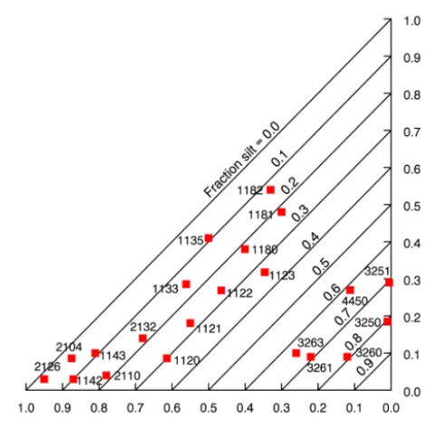
We selected 21 soils from the UNSODA database (Nemes et al., 2001; National Agricultural Library, 2018). The database has relatively many records for sandy soils, and hardly any in heavy clays. The selected soils have no organic matter con-tents that would lead to considering them as organic soils, have texture data records that allow their texture class to be determined, are fairly uniformly distributed over the textures covered by the database, have data points on the main drying curve, and have measurements over a sufficiently wide range of matric potentials to allow retention curves to be fitted to them.
We classified the texture of the selected soils according to the USDA classification as well as the hydrologically ori-ented classification developed by Twarakavi et al. (2010). The latter distinguishes 12 texture classes, grouped in three sets (A, B, C) of four each (1 through 4). Soils with (nearly) 100 % sand, silt, or clay are classified as A1, B1, and C1, re-spectively. Numbers larger than 1 identify texture classes that must have at least two of the components sand, silt, and clay. B3 and C4 are the only categories that must have all three components. The differences with the USDA classification are considerable for clayey and silty soils, and we refer to Twarakavi et al. (2010) for full details. Figure 1 shows the distribution of the selected soils over the soil texture triangle. 3.2 Parameter fitting
3.2.1 Selected parameterizations
[image:7.612.310.545.61.297.2]We fitted the original Brooks–Corey (BCO, Eq. S1a) and van Genuchten (VGN, Eq. S4a) parameterizations, and the derivates thereof that do not lead to unrealistic hydraulic conductivities near saturation: FSB (Eq. S12a) and RNA (Eq. S9a), both of which emerged from BCO, and VGA (Eq. S7a), which emerged from VGN. Thus, BCO, FSB, and
Figure 1.The textures of the soils used to test the fitting capability of selected soil water retention curve parameterizations. The num-bers next to the data points are the identifiers used in the UNSODA database to distinguish individual soils.
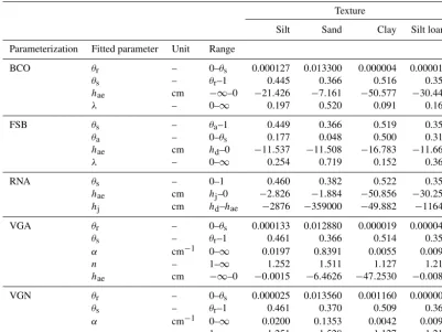
RNA all have a power law shape in the mid-range of the matric potential (and for BCO over the full range below the air-entry value). The slope therefore monotonically increases with decreasing water content. VGN and VGA have a sig-moid shape and therefore are able to fit curves that have an inflection point. As Groenevelt and Grant (2004) pointed out, θr serves as the third required shape parameter for curves with an inflection point, frequently resulting in improbable values for this parameter. Table 1 shows the fitting parame-ters and their physically permitted range.
All three conductivity models are compatible with BCO, FSB and RNA. Burdine’s (1953) and Mualem’s (1976) con-ductivity models can be used with VGA. VGN does not meet the criterion of Eq. (4) but is very often used in conjunction with Mualem’s conductivity model (1976). It was therefore included for comparison.
3.2.2 The objective function and its weighting factors A set of parameters describing the soil water retention curve must be optimized to provide the best fit to an arbitrary num-ber of data points. To do so, an objective function was mini-mized, construed by the sum of weighted squares of the dif-ferences between observed and fitted values. The fitted val-ues depend on the parameter valval-ues in the parameter vec-torx. Assumeqθ observation pairs of water content vs.
ma-tric head (hi,θi). Here,θi denotes theith observation of the
Table 1.The fitting parameters for five parameterizations, their physically permitted ranges, and their fitted values for four textures. The three-character parameterization label is explained in the main text.
Texture
Silt Sand Clay Silt loam
Parameterization Fitted parameter Unit Range
BCO θr – 0–θs 0.000127 0.013300 0.000004 0.000015
θs – θr–1 0.445 0.366 0.516 0.358
hae cm −∞–0 −21.426 −7.161 −50.577 −30.440
λ – 0–∞ 0.197 0.520 0.091 0.163
FSB θs – θa–1 0.449 0.366 0.519 0.358
θa – 0–θs 0.177 0.048 0.500 0.312
hae cm hd–0 −11.537 −11.508 −16.783 −11.668
λ – 0–∞ 0.254 0.719 0.152 0.364
RNA θs – 0–1 0.460 0.382 0.522 0.358
hae cm hj–0 −2.826 −1.884 −50.856 −30.250
hj cm hd–hae −2876 −359000 −49.882 −11641
VGA θr – 0–θs 0.000133 0.012880 0.000019 0.000041
θs – θr–1 0.461 0.366 0.514 0.358
α cm−1 0–∞ 0.0197 0.8391 0.0055 0.0093
n – 1–∞ 1.252 1.511 1.127 1.219
hae cm −∞–0 −0.0015 −6.4626 −47.2530 −0.0081
VGN θr – 0–θs 0.000025 0.013560 0.001160 0.000003
θs – θr–1 0.461 0.370 0.509 0.360
α cm−1 0–∞ 0.0200 0.1353 0.0042 0.0095
n – 1–∞ 1.251 1.528 1.127 1.219
water column), andi∈ {1,2, . . ., qθ}is a counter. In the code,
the assumed units are centimeters of water column forhand cubic centimeters of water per cubic centimeter soil forθ.
The definition of the objective function FR(xp,R)at the
Rth iteration during the fitting operation is as follows: FR(xp,R)=wTθ,Rdθ(xp,R,xf)R∈ {1,2, . . ., Rmax}. (5) Here,dθdenotes a vector of lengthqθof squared differences
between observations and fits that are functions of the fitted parameter valuesxp and the fixed (nonfitted) parameters in
vectorxf. Together,xp andxf constitutex. Each squared
difference is weighted. The weight factor vector is denoted bywθ,R. Its dependence on the water content and iteration
step is explained below. The superscript T indicates that the vector is transposed. To terminate infinite loops, the number of iterations is capped byRmax.
For relatively wet soils (0 >h>−100 to−200 cm), mea-surement methods are available that create a hydrostatic equilibrium in a relatively large sample. In such caseshi re-flects the matric potential at the center of the sample butθi is
that determined for the entire sample. The vertical variation of hresults in a nonuniform water content, and the average water content of the sample (θi)may not be well represented
by the water content corresponding tohi. For these cases, the height of the sample can be specified on input. The code then
divides the sample into 20 layers, calculateshin the center of each layer, computes the corresponding water contents from
xp,R, and averages these to arrive at an estimate ofθi.
If and only if the standard deviation of the measurement error of the individual observations is known, a maximum-likelihood estimate of the soil hydraulic parameters can be obtained (Hollenbeck and Jensen, 1998). To ensure this, the weighting factors in vectorwθ,Rmust be equal to the
parameter values through the iterative process. Low informa-tion content (indicated by large random fluctuainforma-tions of a pa-rameter value), correlated papa-rameters, and papa-rameters trend-ing towards a minimum or maximum permitted value can usually be diagnosed from such records.
Data points for a retention curve over the whole moisture range cannot be obtained by a single method. Furthermore, measurement errors occur in bothhiandθi. To accommodate
this, the error standard deviationsσh,iandσθ,i forhandθ,
respectively, can be provided individually for any data point i. To improve the performance of the fitting routine, the val-ues ofσθ,iare scaled to ensure their average equals 0.20, i.e.,
the same order of magnitude asθ. The values ofσh,iare then
scaled by the same scaling factor. The weighting factorwR,I
for observationθi during iterationRis as follows:
wR,i=σi,R∗
−2= σ∗
h,i
dθ dh
R,i
+σθ,i∗
!−2
, (6)
where the asterisk denotes a scaled value. The subscriptsi andRlabel data points and iteration steps as above. The gra-dient is determined from theRth fittedθ (h)relationship de-fined by xp,R. Thus, the weighting factors are updated for
every iteration.
In the code, the gradient is approximated by 1θ / 1h computed from the water contents at hi±max(1 cm H2O, 0.01·hi). For data points acquired at hydrostatic equilibrium, this would require 40 additional calls to the function that computes the θ corresponding to a given value ofh, which would be rather inefficient. Instead, the water content is cal-culated for one virtual layer below and one above the sample. By subtracting the water content of the top (bottom) layer in the sample and adding the water content of the virtual layer below (above) the sample, the water content corresponding tohi+H /20 (hi−H /20) can be found, withH the sample height in centimeters. In this way,1θ / 1hcan be computed with only two additional calls to the function that defines the parameterizedθ (h)relationship.
3.2.3 Parameter optimization by shuffled complex evolution (SCE)
The calibration algorithm employed here is the shuffled com-plex evolution algorithm introduced by Duan et al. (1992) with parameter adjustments of Behrangi et al. (2008). The strategy of this algorithm is to form out ofj+1 parameter sets, wherej is the number of model parameters, so-called complexes (e.g., triangles in 2-D). Each vertex of the com-plex not only represents one of thej+1 parameter sets but also the model’s skillFR(xp,R)to match the observed data
when it is forced with the according parameter setxp,R. This
skill is usually referred to as the objective function value of an objective to be minimized. The vertex with the worst skill or largest objective function value is subsequently perturbed in order to find a better substitute parameter set. This strategy
is repeated until the volume of the complex, i.e., the agree-ment of the parameter sets, is smaller than a threshold. To avoid that, the search gets stuck in a local optimum, and a number ofY complexes are acting in parallel. After a certain number of iterations theY·(j+1) vertexes are shuffled and newly assigned to Y complexes. The algorithm converges when the volume of all complexes is lower than a threshold which means that allY·(j+1) vertexes are in close prox-imity to each other. Infinite runs of the SCE are avoided by Rmax, but convergence should be the desired target for termi-nation of the SCE.
The SCE algorithm used here is configured with two com-plexes each consisting of (2j+1) ensemble members. The different parameterizations we fitted had 3 to 5 fitting pa-rameters. In each iteration,j+1 parameters are randomly selected and the vertex with the worst skill is perturbed. The reflection and contraction step lengths in the Simplex method (e.g., Press et al., 1992, pp. 402–404) were set to 0.8 and 0.45, respectively. SCE seems to have an order of about O(j2). In our case it required between roughly 250 and 3000 model evaluations to find the optimal parameter set. For each parameter estimation run, three sets of initial guesses of the fitting parameters must be provided. The results of the three trials were compared to reduce the chance of accepting a lo-cal minimum of the objective function. The selection of SCE was based on its widespread usage in hydrological studies and according to a preliminary experiment where the SCE outperformed other algorithms like the simulated annealing (Kirkpatrick et al., 1983) and the Dynamically dimensioned search algorithms (Tolson and Shoemaker, 2007) in optimiz-ing more than 80 analytical test functions with j ranging from 2 to 30.
3.3 Scenario study by numerical simulations
As stated in the Introduction, previous tests of parametric ex-pressions of soil water retention functions mostly focused on the quality of the fit to direct observations of points on the water retention curve. Here, we will also examine how the various parameterizations affect the solution of Richards’ equation by simulating water fluxes and soil water profiles for a scenario involving infiltration and evaporation. We set up a hypothetical 999-day scenario representative of a desert climate with prolonged drying, infiltration into dry soil, and redistribution after rainfall, permitting a comprehensive test of the parameterizations. We used the HYDRUS 1-D model version 4.xx (Šim˚unek et al., 2013, http://www.pc-progress. com/en/Default.aspx?hydrus-1d) to solve Richards’ equation in a 1-D soil profile. We permitted flow of liquid water as well as diffusive water vapor fluxes.
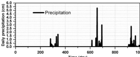
Figure 2.The record of daily rainfall sums from Riyadh city that was used in the numerical scenario study. Three rainfall clusters are visible. The largest daily rainfall amount (5.4 cm) fell on day 656. The observation period starts on 4 June 1993, and ends on 27 February 1996.
drainage immediately after the start of the simulation as the lowest part of the profile adapted to the unit gradient conditions in the two lowest nodes that the free drainage condition imposed. The upper boundary conditions were atmospheric (during dry periods: prescribed matric poten-tial set to −50 000 cm; during rain: prescribed flux density equal to the daily rainfall rate derived from observed daily sums). The weather data (daily rainfall and temperature) were taken from the NOAA database (http://www.ncdc.noaa. gov/cdo-web/, National centers for environmental informa-tion, 2017) for a station in Riyadh city (Saudi Arabia) be-tween 4 June 1993 and 27 February 1996. In this period, spanning nearly 3 years, there were three clusters of rain-fall events (Fig. 2). The second cluster was the heaviest with a maximum daily sum of approximately 5.4 cm on day 656. A prolonged dry spell preceded the first rainfall cluster. We used the first 250 days of this period as a “burn-in” period to minimize the effect of the initial condition on the calculated fluxes. This leaves a period of 751 days for analysis.
The simulation period involved large hydraulic gradients when water infiltrated a very dry soil, limited infiltration of small showers followed by complete removal of all water, and deeper infiltration after clusters of rainfall that deliv-ered large amounts of water followed by prolonged periods in which flow of liquid water and water vapor occurred si-multaneously. These processes combined permitted a com-prehensive comparison of the various parameterizations. We were interested in the magnitude of the fluxes of liquid water and water vapor and the partitioning of infiltration into evap-oration, storage change, and deep infiltration under various conditions, and the effect on these fluxes and storage effects of the choice of parameterization. We did not intend or de-sire to carry out a water balance study. Under semiarid condi-tions this would have required a much longer meteorological record, which was not available.
The various parameterizations are not implemented in HY-DRUS. We therefore used the MATER.IN input file to sup-ply the soil hydraulic property curves in tabular form to the model. The retention models BCO, FSB, and RNA
permit-ted all three conductivity models (Burdine, B; Mualem, M; and Alexander and Skaggs, AS) to be used. VGA only gives useful expressions for Burdine and Mualem. VGN only al-lows Mualem’s conductivity model. Thus, there are 12 com-binations of retention and conductivity curves that we tested on four different textures, leading to 48 different simulations (and MATER.IN files) in total.
4 Results and discussion
4.1 Fitted parameters and quality of the fits for the soils used in the simulations
Table 1 presents the fitted parameters for all combinations of texture and parameterization for the soils used in the simula-tions. The parameter with the best-defined physical meaning isθs. All parameterizations give comparable values for it for each texture, which reflects the relatively narrow data clouds near saturation. The values ofθr are relatively high for the three parameterizations in which it occurs. The air-entry val-ues (hae)should increase (move closer to zero) from clay to silt loam to silt to sand, which is the case for BCO, FSB, and RNA, but not for VGA. The data in Fig. 3 support rel-atively similar values for all textures other than clay, which is somewhat surprising. RNA gives rather high values in silt and sand, and VGA does very poorly in sand and silt loam. The high value forhaefor FSB in clay may be related some-how to the very high value of the maximum adsorbed water contentθa, which we fixed close toθs. The value ofθafor clay should be larger than that for silt loam, so it cannot be more than about 0.2 off though. The spread ofhjfor RNA across the textures show that this parameter needs to be allowed to be fitted over its full range (betweenhdand at least the mini-mum value ofhae). Even with initial guesses that differed by several orders of magnitude, the fits were still quite consis-tent, so evidently these values are supported by the data and not an artefact.
In 3 of the 48 parameter estimation runs, the fits pushed one of the parameters to one of its bounds (even after ex-panding these to their physical limits), irrespective of their initial guess: FSB for clay (we fixedθato 0.5), VGN for sand, and RNA for silt (we fixedθson the basis of the data in both cases). For BCO and VGA in sandy soil, the code could not converge to a global minimum, indicated by the volume of the complexes, which exceeded the threshold. The fitted pa-rameters should be viewed critically in these two cases.
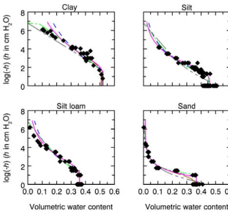
Figure 3.Observed and fitted retention curves for the different soil textures.
Table 2.Root mean square errors (RMSEs) for the different param-eterizations.
Texture
Parameterization Silt Sand Clay Silt loam
BCO 0.1422 0.1164 0.1858 0.1122
FSB 0.1248 0.1163 0.1205 0.1068
RNA 0.0341 0.0130 0.2192 0.1101
VGA 0.0118 0.1164 0.1604 0.0412
VGN 0.0118 0.0111 0.1547 0.0411
in the RMSE values between textures reflects the different scatter in the underlying data clouds.
The soil water retention curves defined by the different pa-rameterizations are plotted in Fig. 3. The models that were not developed with dry conditions in mind (BCO, VGA, and VGN) have relatively high water contents in the dry end of clay and silt loam. The logarithmic dry end of FSB and RNA eliminates this asymptotic behavior. The cutoff to zero of the FSB parameterization is quite strong in fine-textured soils. The fixed value ofhd (where the water content is zero) of RNA seems to be too small for clay while appearing to be adequate for the other textures.
In the intermediate range, all fits are close to one another. RNA underperforms in sand and silt compared to the others. In the wet range, the absence of an air-entry value in VGN results in a poor fit for sand. Here, the contrast between VGN and VGA is very clear. Overall, the inclusion of the water-entry value as a parameter seems beneficial to the fits. FSB has the most satisfactory overall performance.
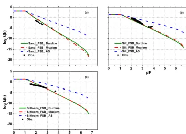
For sand, silt, and silt loam, independent observations of K(h) were available. The fits of Burdine’s (1953) and Mualem’s (1976) parameterizations based on retention data only were remarkably good for all parameterizations. The function of Alexander and Skaggs (1986) severely overes-timated the hydraulic conductivity in all three cases, but very accurately described the slope of the curve for silt loam. Fig-ure 4 demonstrates this for FSB, and the results for the other parameterizations were comparable.
4.2 Simulation results
For all simulations, the vapor flux within the profile was of little consequence compared to the liquid water flow. For that reason it will not be discussed in detail here. Vapor flow may play a larger role under more natural conditions with day– night temperature cycles and in the presence of plant roots. 4.2.1 Silt
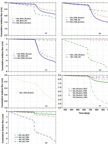
We start the analysis by examining the flux at the bottom of the soil profile. Figure 5a–e shows all combinations of pa-rameterizations of the retention and conductivity curves.
The early rainfall cluster event at aroundt=300 days did not generate any bottom flux, and therefore only wetted up the soil profile. In doing so it increased the effect of the heav-ier rainfall aroundt=656 days on the bottom flux.
For the individual parameterizations, Mualem and Burdine gave reasonably similar results in which the second and third rainfall cluster generated a little more downward flow for B than for M. In all cases, Alexander and Skaggs gave a more rapid response of a very different magnitude. Clearly visible is a sustained, constant flux leaving the column during pro-longed dry periods for the AS conductivity curves. This is physically implausible.
Figure 5f shows the substantial effect of the parameteri-zation of the water retention curve on bottom fluxes when the M-type K(h) function is deployed. The results for B-typeK(h)were comparable. Different retention curves gave very different responses to the initial conditions (not shown), highlighting the need to add a sufficiently long lead time ahead of the target time window to the simulated time period. RNA’s response to the second and third rainfall clusters was about 2.4 times that of the others. Ath= −300 cm (pF 2.48), Kaccording to M is at least 5 times higher for RNA than for the rest, while the water content at that matric potential and higher values is relatively small (Fig. 3c). Thus, infiltrated water was transported downward with relative ease, giving rise to the relatively high bottom fluxes and low evaporation rates that were computed for RNA (Figs. 5f, 6f). The param-eterizations other than RNA behaved rather similarly, except for the fact that VGA responded much faster to a change in the forcings than the other parameterizations.
[image:11.612.52.283.370.467.2]rain-Figure 4.The observed and fitted hydraulic conductivity curve according to Burdine (1953), Mualem (1976), and Alexander and Skaggs (1986) using the fitted parameters of the Fayer and Simmons soil water retention curve (1995) for(a)sand,(b)silt, and(c)silt loam. The units ofKare centimeters per day (cm d−1).
fall was very fast and short-lived, which seems improbable for a silt soil that is far from full saturation. The nonphysi-cal bottom flux during dry periods (especially for VGA), the slow calculation times (half as fast as the others) with the time step always at the smallest permitted value, and non-negligible mass balance errors all point to numerical prob-lems associated with AS.
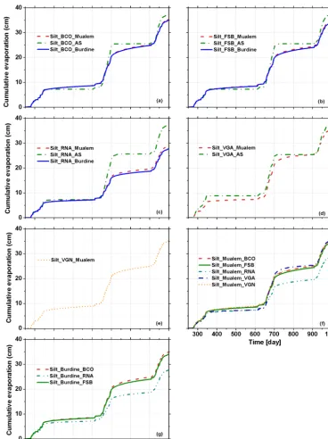
The evaporative flux was nearly identical for B and M con-ductivity functions (Fig. 6a–c). Since their bottom fluxes dif-fered, this necessarily implies that the storage in the soil pro-file must also be different for B and M. The AS parameteri-zation gave a much more spiky response of evaporative flux to rainfall than B or M, with zero evaporation most of the time (Fig. 6a–d). In terms of cumulative evaporation, AS re-sponded more strongly to the second rainfall cluster around t=650 days (Fig. 6a–c). Overall, the effect of the conduc-tivity function on the relative differences in evaporation was less pronounced than on the relative differences in the bottom flux. The same was true for the parameterization of the reten-tion curve, as demonstrated by the relatively similar shapes of the curves in Fig. 6f and g.
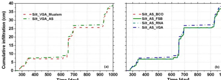
Given the nonphysical behavior of the bottom flux of AS for VGA in particular (Fig. 5d), we also examined the infil-tration. We first compare infiltration for VGA with M- and AS-type conductivity (Fig. 7a) and clearly see the zero infil-tration for VGA during periods without rain contrasted to the impossible nonzero infiltration rates for AS during dry spells.
For the other water retention parameterizations in combina-tion with AS, the effect is less pronounced (Fig. 7b). Still, the AS conductivity should be used with care and the results and mass balance checked.
Table 3 summarizes the bottom and evaporative fluxes. For evaporation, the differences are inconsequential except for the markedly low values for RNA. For the bottom flux, the difference between B and M is small enough to be within the margin of error for typical applications. The effect of the pa-rameterization of the retention curve is an order of magnitude between the smallest bottom flux (for VGA) and the largest (for RNA).
4.2.2 Sand
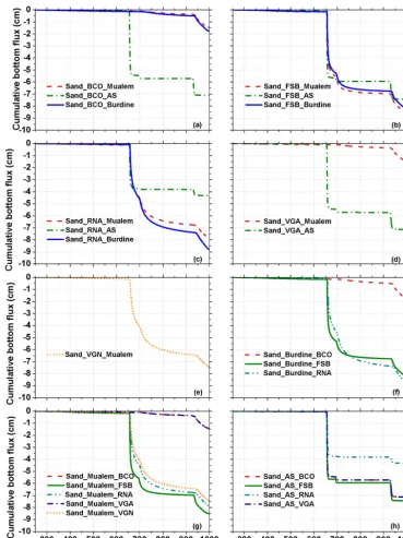
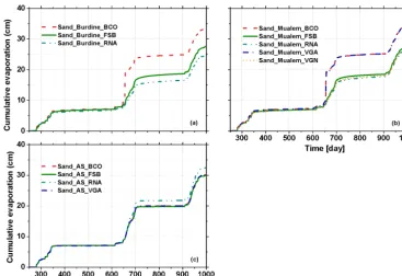
The relationship between the bottom (Fig. 8) and evaporative fluxes (Fig. 9) as generated by the various parameterizations for the sandy soil were comparable to those for silt, and the analysis applied to the silt carries over to sand. The bottom fluxes in sand responded faster and with less tailing than in silt, and the third rainfall cluster near the end of the simula-tion period produced a clear signal (Fig. 8).
[image:12.612.114.481.60.324.2]Figure 5.The cumulative bottom fluxes leaving a silt soil column for the different combinations of soil water retention curve and hydraulic conductivity parameterizations. Panels(a)through(e)present the results for the indicated retention parameterizations (see Table 1). Panels(f, g)organize the results according to the conductivity function: either Mualem (1976)(f)or Alexander and Skaggs (1986)(g).
The bottom fluxes for BCO and FSB with AS-typeK(h) are similar (Fig. 8h), in stark contrast to the bottom fluxes based on B (Fig. 8f) and M (Fig. 8g) for these parameteri-zations. The similarity in the fluxes for AS reflect the facts that the evaporative fluxes (occurring in the wet range, where BCO and FSB both have Brooks–Corey retention curves) are very similar and the spiky response typical for AS results in only a small difference in storage between BCO and FSB.
Consequently, the bottom flux, as the only remaining term of the water balance, cannot differ strongly between BCO and FSB. The difference in the bottom fluxes generated for VGN and VGA with M-typeK(h)(Fig. 8g) is even more extreme than in case of the silty soil.
dif-Figure 6.Cumulative evaporation from a silt soil column for the different combinations of soil water retention and hydraulic conductivity parameterizations. Panels(a)through(e)present the results for the indicated retention parameterizations (see Table 1). Panels(f, g)organize the results according to the conductivity function: either Mualem (1976)(f)or Burdine (1953)(g).
ferences seem to have been dominated by the complemen-tary responses of evaporation and bottom fluxes to the rain-fall events aroundt=656 days. BCO converted roughly 5– 7 cm more of this rainfall to evaporation than the other pa-rameterizations, for both B and M. Therefore, less water was available for downward flow, resulting in a cumulative
bot-tom flux for BCO that was roughly 6 to 8 cm smaller than for the other parameterizations.
[image:14.612.114.482.65.557.2]Figure 7. Cumulative infiltration in a silt profile for the VGA parameterization (see Table 1) with conductivity functions according to Mualem (1976) and Alexander and Skaggs (1986)(a)and four different parameterizations for the retention curve (see Table 1) with the Alexander and Skaggs conductivity function(b).
Table 3.Cumulative bottom and evaporative fluxes (positive upwards) for silt from day 281 (the start of the first rainfall) onwards for Burdine and Mualem conductivity functions with the different parameterizations. The hydraulic conductivity ath= −300 cm (the initial condition at the bottom) is also given.
Cumulative bottom flux (cm) Cumulative evaporation (cm) K(−300) (cm d−1)
Parameterization Burdine Mualem Burdine Mualem Mualem
BCO −0.70 −0.500 34.147 34.445 0.00080
FSB −1.240 −0.910 33.219 33.736 0.00147
RNA −4.337 −3.650 27.046 28.184 0.00702
VGA – −0.248 – 34.956 0.00014
VGN – −0.744 – 34.359 0.00119
considerably smaller for RNA than for the other parameteri-zations.
Coarse-textured soils have the sharpest drop in the hy-draulic conductivity as the soil desaturates. We therefore used the result for the sandy column to study the relationship between the matric potential at the bottom of the column and the bottom flux in order to evaluate water fluxes in dry soils. The free drainage lower boundary condition ensures there is always a downward flux that is equal to the hydraulic conduc-tivity at the bottom at any time. Particularly for coarse soils this can still lead to negligible bottom fluxes for considerable periods of time. We first consider FSB and RNA, these being the parameterizations specifically developed to perform well in dry soils.
The difference in matric potentials between FSB and RNA is immediately clear from Fig. 10a, b and 11a, b. The ef-fect of the conductivity function is manifest by including Figs. 10c and 11c in the comparison. The effect of the first rainfall cluster is visible in the matric potential in all cases (Figs. 10 and 11), but not enough to generate a significant flux. A flux through the lower boundary first occurs when the matric potential there exceeds (i.e., becomes less nega-tive than)−70 cm for FSB (Fig. 10a and b) and−30 cm for RNA (Fig. 11a and b).
The second rainfall cluster at 600 <t< 700 days did not rely on prewetting: it produced a bottom flux no matter how dry the soil was. The third rainfall cluster around day 930 probably would not have generated a bottom flux for B- and M-typeK(h)functions, had the previous rainfall cluster not prewetted the soil. Note that the previous rainfall affects ma-tric potentials at 1 m depth for several hundreds of days for B-and M-type conductivity functions, but only for a few months at most for AS.
The AS-typeK(h)function gave such rapid responses that only the second flux event at about 694 days was a result of recent prewetting att≈656 days (Figs. 10c and 11c). De-spite the very different matric potentials at the bottom, the cumulative bottom fluxes produced by a single rainfall clus-ter generated by FSB and RNA were quite similar for B and M and only somewhat larger for AS (Figs. 10 and 11).
The AS conductivity function led the soil to dry out so completely that the atmospheric matric potential during dry spells was reached at 1 m depth in a few months (Figs. 10c and 11c). This seems unrealistic, and seems to be related to the significant overestimation of the unsaturated hydraulic conductivity by AS evidenced in Fig. 4.
Figure 8.As in Fig. 5, but for a sandy soil column. Unlike Fig. 4, the results of Burdine’s (1953) conductivity curve are shown(f).
poor fitting performance, probably incorrect. The differences between the parameterizations illustrate the need to carefully consider the suitability of the parameterization for the in-tended purpose.
4.2.3 Silt loam and clay
The bottom fluxes from the clay and the silt loam soil for all combinations of parameterizations for the soil water reten-tion and hydraulic conductivity curves were similar to those
Figure 9.Cumulative evaporation from a sandy profile for the different combinations of retention curve parameterizations (see Table 1) and hydraulic conductivity functions: Burdine (1953)(a), Mualem (1976)(b), or Alexander and Skaggs (1986)(c).
The behavior of the evaporative fluxes from the silt loam and the clay soil for all combinations of parameterizations for the soil water retention and hydraulic conductivity curves was essentially similar to that for the silty soil (Figs. 14 and 17). The main difference was the less gradual response of the evaporation for VGA, particularly for clay, which was, in fact, rather similar to the notoriously spiked response of the AS-type conductivity function. The relative amounts of evaporation of the various parameterizations varied from one texture to another.
For AS in combination with the VGA retention curve, there was significant infiltration during periods of zero rain-fall (Figs. 15 and 18). This numerical artefact led to erro-neous simulations of the bottom flux. This is the most signif-icant occurrence of mass balance errors that plague the sim-ulations with AS-typeK(h)functions in silt loam and clay, as they did in silt. Evidently, the AS parameters for theK(h) curve cause numerical problems in fine-textured soils. 4.3 Fits for a wide range of textures
The fits for the clayey soils selected from the UNSODA database (Fig. S1, first panel) show that with data ranging to pF≈4, data points in the drier region would have helped guide the fitting process. VGA and VGN produced good fits but struggled with high residual water contents, as did BCO. We modified FSB by requiring that the capillary-bound water content goes to zero when the adsorbed water content does, a modification of the original equation by Fayer and
Sim-mons (1995). The cutoff value of the matric potential was clearly too small for these fine-textured soils, and an unre-alistic jump to zero water content occurred for the C2 and C4 soils with nos. 1122, 1123, 1135, 1181, and 1182 in the UNSODA database. database. The matric potential at oven dryness evidently needs to be extremely low for soils with high clay content.
Rossi and Nimmo (1994) fixed the matric potential in their parameterization at which the water content became zero. The fits for the soils used in the simulations showed that fix-inghdfor RNA did not always give satisfactory fits in the dry range, and we therefore madehda fitting parameter. Supple-ment Fig. S1 (first panel) shows that this parameter may need a large lower boundary, similar to FSB: the maximum value (pF=10) still gave poor fits for some of the fine-textured soils (soils with nos. 1122 and 1123, both C4 in Twarakavi et al.’s (2010) classification, in which the category is centered roughly around the point where sand, silt, and clay all con-tribute one-third to the total mineral soil).
Figure 10.Pressure head hBot and flux density vBot at the bot-tom of the sand column for the FSB parameterization (see Ta-ble 1) and the conductivity functions of Mualem (1976)(a), Bur-dine (1953)(b), and Alexander and Skaggs (1986)(c).
the quality of the fit, the fitted parameter values can no longer be qualified as maximum likelihood estimates.
For silty soils (Fig. S1, second panel), the fits were gener-ally good, with some evidence that the fitted residual water contents were somewhat high for some soils (3260, 3261). The extrapolations to zero water content by FSB and RNA appeared plausible even though they differed significantly in some cases (3251, 4450), highlighting the desirability of data points in the dry range.
[image:18.612.326.527.69.447.2]For sandy soils with some clay and/or silt (A3 and A4, Fig. S1, third panel), residual water contents for BCO, VGN, and VGA were often large (1120, 1143, 2110, 1133). When the data range was limited (below pF≈4), considerable ex-trapolation was required. In most cases, FSB and RNA did so better than VGN and VGA. If there is a discrepancy be-tween the porosity and near-saturated water contents (1121, 1143, and 2110), BCO and FSB tended to shift their saturated
Figure 11.As in Fig. 10, but for the RNA parameterization (see Table 1).
branches towards the porosity, because of the higher weight assigned to this data point.
For sandy soils (A1 and A2, Fig. S1, fourth panel), the fits were good if the data covered the full water content range. In all cases, VGA and VGN fitted the residual water content close to driest data point, which is very unrealistic if the dry range was not covered (1142).
Figure 12.As in Fig. 10, but for the BCO parameterization (see Table 1).
For the fits of the four soils used for the simulation and the 21 soils, sets of three optimizations were independently run for all five parameterizations, with initial guesses that cov-ered the full range over which the parameters were allowed to vary. In about a quarter of the cases we found no more than a single acceptable fit, and we ran these again with other sets of initial guesses (again widely different from one another) and/or expanded parameter ranges. For only two of the 125 fitted parameter sets did this procedure not lead to convincing convergence.
In none of the cases did the three independent runs yield parameter estimates that differed by more than 10 % while the sum of squares of the fits differed by less than 10 %, even though in all cases the initial guesses were very differ-ent, thereby ensuring that the starting points of the different searches were located in completely different regions of the parameter space. We take this as evidence of the absence of parameter correlations, since one would expect correlated pa-rameters to vary over a considerable range, with the RMSE of different combinations of parameter values remaining nearly constant. We found that the fitted values obtained from the different runs were very similar, with an occasional outlier in a local minimum with a considerably larger RMSE.
In order to determine the correlation matrix of the fitted pa-rameters correctly, a Markov Chain–Monte Carlo approach would be required for each of the 125 combinations of soils and parameterizations. Given the lack of evidence that
signif-icant correlations exist, we considered this beyond the focus of and the computational resources available for this work.
Some of the data sets displayed multimodality. None of the parameterizations we tested can account for that, which is why we did not examine this further in this paper. If one wishes to reproduce this by summing several curves of the same parameterization but with different parameter values (advocated by Durner, 1994), one needs a sigmoidal curve. If physically realistic conductivity curves near saturation are deemed desirable, VGA is the only viable parameterization for this purpose among those evaluated in this paper. 4.4 General ramifications
We found that 14 out of 18 parameterizations of the soil water retention curve were shown to cause nonphysical hydraulic conductivities when combined with the most popular (and effective) class of soil hydraulic conductivity models. For one of these cases (VGN), Ippisch et al. (2006) demonstrated convincingly that their alternative (VGA) significantly im-proved the quality and numerical efficiency of soil water flow model simulations, and our simulations confirmed the pro-found effect of this modest modification on the model results. We hope that the general criterion we developed for verifying the physical plausibility of the near-saturated conductivity will be used in the selection of suitable soil hydraulic prop-erty parameterizations for practical applications of numerical modeling of water flow in soils, and likewise will be of help in improving existing parameterizations (as we have done in a few cases here) and developing new ones.
Replacing the residual water content in a retention curve parameterization by a logarithmic dry branch generally im-proved the fits in the dry range for many soils. If data in the dry range were lacking, the logarithmic extension provided a physically realistic extrapolation into the dry range, but the spread between the different fits showed the level of uncer-tainty in this extrapolation caused by the limited range of the data. The cutoff to zero water content of FSB could be ex-cessive for fine-textured soils, but this is only a problem if the soil actually so far that it reacheshd. For RNA, adequate fits in the dry range require that the matric potential at which the water content reaches zero is to be treated as a fitting parameter. With the added flexibility of this fourth fitting pa-rameter, RNA emerged as a very versatile parameterization, producing mostly good fits for a wide range of textures. Nev-ertheless, its lack of an inflection point was occasionally a limitation.
Figure 13. Cumulative bottom fluxes from a silt loam profile for all combinations of parameterizations (see Table 1) and Mualem’s (1976)(a)and Alexander and Skaggs’ (1986) conductivity functions(b), and for the RNA parameterization with all three conduc-tivity functions(c).
Figure 14. Cumulative evaporation from a silt loam profile for all parameterizations (see Table 1) with Mualem’s (1976) conductivity function(a)and the VGA parameterization with conductivity functions according to Mualem (1976) and Alexander and Skaggs (1986)(b).
This resulted in a rapid and unrealistically strong response to changes in atmospheric forcings even at 1 m depth, as shown in our simulation study.
The simulations with different parameterizations showed that under the given boundary conditions the choice of the parameterization had a modest effect on evaporation but strongly affected the partitioning between soil water storage and deep percolation. The uncritical use of a default soil hy-draulic parameterization or selection of a parameterization solely based on the quality of the fit to soil water reten-tion data points entails the risk of an incomplete apprecia-tion of the potential errors of the water fluxes occurring in the modeled soil. This points to the importance of carefully
[image:20.612.116.481.378.510.2]Figure 15.Cumulative infiltration from a silt loam profile for four parameterizations (see Table 1) with the Alexander and Skaggs (1986) conductivity function(a)and for the VGA parameterizations with conductivity functions according to Mualem (1976) and Alexander and Skaggs (1986)(b).
Figure 16.As in Fig. 13, for clay.
[image:21.612.111.484.563.693.2]Figure 18.As in Fig. 15, for clay.
expressions of interest in the numerical solvers of Richards’ equation capable of running in parameter estimation mode.
Code and data availability. The parameter optimization code is