7007
GRADIENT BASED OPTIMIZATION IN CASCADE
FORWARD NEURAL NETWORK MODEL FOR SEASONAL
DATA
1BUDI WARSITO, 2RUKUN SANTOSO, 3HASBI YASIN, 4SUHARTONO
1,2,3Department of Statistics, Diponegoro University, Semarang, INDONESIA
4Department of Statistics, Institute of Technology of Sepuluh November, Surabaya, INDONESIA
E-mail: 1[email protected], 2[email protected], 3[email protected],
ABSTRACT
Optimization technique is an important part in neural network modeling for obtaining the network weights. The choosing a certain optimization method would influenced the prediction result. Many gradient based optimization methods have been proposed. In this research, we applied the three optimization techniques for obtaining the weights of Cascade Forward Neural Network (CFNN), they were Levenberg-Marquardt, Conjugate Gradient and Quasi Newton BFGS. In CFNN, there are direct connection between input layer and output layer, beside the indirect connection via the hidden layer. The advantage is that this architecture allows the nonlinear relationship between input layer and output layer by not disappear the linear relationship between the two. The proposed model was applied in the time series data with the seasonal pattern. The two data types were used to select the most appropriate optimization method for seasonal series. The first type was the generated data from seasonal ARIMA model and the second was the rainfall data of ZOM 145 at Jumantono Ngadirojo Wonogiri. After processing the proposed methods by using Matlab routine we recommended to use the Levenberg Marquardt as the chosen one.
Keywords: CFNN, Gradient, Optimization, Seasonal, Rainfall
1. INTRODUCTION
Time series data relating to season effects are strongly influenced by climate change. Climatic and weather forecasting technologies through a stochastic approach such as time series and regression models have grown quite rapidly, as the circulation models are drawn up by the laws of physics and expressed in terms of mathematical equations that identify relationships between various climate variables such as temperature, air pressure, wind, and rain. The mainly growing stochastic models were nonparametric models, include neural network [1-5]. Predictive models based on statistical approaches are continuously
developed to obtain model specifications
appropriate to the research location.
Neural network modeling has progressed rapidly along with developments in the computing field. Many studies have been conducted in various real problem and also various types of data, including for forecasting of time series data. Some studies that use the neural network model for time series prediction are [6-9]. Several studies have also been
conducted related to NN modeling for seasonal time series. Cigizoglu et al. [10] conducted a comparison of several NN models on rainfall data in Turkey while Benmahdjouba [11] implemented the Feed Forward Neural Network (FFNN) model for rain forecast in Algeria. Some of the other studies are [12-14]. The special class of the FFNN model is the Cascade Forward Neural Network (CFNN). In this class, there is a direct connection between the input and output besides the indirect relationship through the hidden layer [15-16]. Some studies related to the CFNN model for time series are [17-21]. Comparisons of the two architectures, CFNN and FFNN, also have been done [22-24]. Badde et al [25] compared the prediction of compressive strength of ready mix concrete whereas Al-Batah et al [26] applied at the landslide occurence prediction.
7008 [28] proposed a modified conjugate gradient formula for backpropagation neural network algorithm, whereas Apostolopoulou et al. [29] used the BFGS method for neural network training algorithm. With the intention of comparing some gradient-based methods, in this study we used the three of them for obtaining the optimal weights of neural network, they were Conjugate Gradient, Quasi Newton BFGS and Levenberg Marquardt. Comparison of the effectiveness of each method was observed by repeating the same procedure in the same case. The statistics of mean and variance were used to made the conclusion about the most effective one. This is the main motivation of the research objectives undertaken. In many previous studies, the gradient-based optimization methods have been applied to neural networks with the type of FFNN. In this research, the Cascade Forward Neural Network (CFNN) architecture was chosen. The existence of a direct relationship between input and output, in addition to the indirect relationship through the hidden layer, becomes the basis for the selection of this architecture. The proposed method was applied in the both simulation and real problem of seasonal data.
2. MATERIAL AND METHODS
2.1 Cascade Forward Neural Network
Cascade Forward Neural Network (CFNN) is similar to Feed Forward Neural Network (FFNN) but include a weight link between input layer and output layer. The equations are formed from the CFNN model can be written as follows:
(1)
where fi is the activation function from the input
layer to the output layer and is weight from the
input layer to the output layer. If a bias is added to the input layer and the activation function of each neuron in the hidden layer is fh then equation (1)
becomes:
(2)
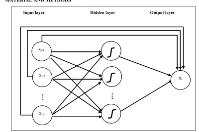
In the CFNN model which is applied in time series data, the neurons in the input layer are the lags of time series xt-1, xt-2, ..., xt-p, whereas the
output is the current data xt. The architecture of
[image:2.612.98.498.428.695.2]CFNN model in predicting time series is shown at Fig. 1.
Figure 1: Architecture of CFNN for time series prediction
xt-1
xt-2
xt-p
xt
7009 The consequence is that the network weight to be estimated increases as much as the neurons in the input layer. Cascade Forward backpropagation algorithm is also similar with Feed Forward backpropagation. As with FFNN, backpropagation algorithm on CFNN also consists of three stages: feedforward of the input pattern, error counting and weight adjustment. Error calculation process is done after the feedforward stage. The updating of network weights is done until no error occurs or until iteration stops, according to the specified stop criteria. In this section we briefly discuss the three optimization methods used in this research.
2.2 Gradient Based Optimization Methods
As with FFNN, backpropagation algorithm on CFNN also consists of three stages: feedforward of the input pattern, error counting and weight adjustment. As explained before, after the feedforward stage the process continues with the error calculation (the difference from the output to the target). The next step is to update the weights and do the recalculation. This step is done until no error occurs or until iteration stops according to the specified stop criteria. In this section we briefly discuss the three gradient based optimization methods for weighting adjustments of the CFNN model, they are conjugate gradient, Quasi Newton BFGS and Levenberg-Marquardt. The systematic stages of each method for function optimization have been explained by Chong and Zak [30].
2.2.1 Conjugate Gradient
Suppose that belonging to a weight vector ω of length s is the set of all network weights and
the objective function is . Defined
Q is the positive-definite matrix of size s×s where QT = Q. Stages of the algorithm on Conjugate Gradient optimization are described as follows:
1) Set k = 0, select the initial point
2) Calculate the gradient of the initial weight
If g(0) = 0 then stop, and it obtained the optimal
weight = . Else, set d(0) = g(0).
3) Calculate
4) Calculate = + d(k)
5) Calculate , if stop
and the optimal weight is
6) Calculate
7) Calculate d(k+1) = -g(k+1) + d(k)
8) k = k+1; go to step 3
As in FFNN, the iteration process for weight searching on CFNN is usually called the epoch. Suppose that the maximum number of permitted epochs is K, if the iteration termination criterion has not been met until epoch k = K then the iteration process will be stopped. On the optimization problem of the general nonlinear model, this algorithm will not always reach convergent in n steps so that the direction vector is re-initialized after a certain iteration and continued until the termination criterion. In the nonlinear model, matrix Q is a non-constant Hessian matrix and evaluated on each iteration. To avoid complicated calculations, elimination of Q is done so that the algorithm depends only on the function and the gradient value of each iteration. There are several formulas for substituting the form of Qd(k) with other forms, such as the Hestenes-Stiefel formula, i.e the form Qd(k) is replaced by
. By this formula the becomes:
The obtaining of optimal weights is done in each epoch.
2.2.2 Quasi Newton BFGS
Weight adjustment on the Quasi Newton BFGS method (Broyden, Fletcher, Goldfarb and Shanno) uses the basic concepts of the Newton
method, where
is a
7010 vector of length p, is the gradient vector and H is
the Hessian matrix which is the second derivative of to ω. To avoid complex calculations, the Hessian matrix is determined iteratively on each epoch by giving initials at the beginning of the training. The initial matrix chosen is a symmetric
positive-definite matrix with the size of , in this case
the commonly used is the identity matrix, H = I. The stages of the optimization algorithm in the Quasi Newton BFGS method are described as follows.
1) Set k = 0, select the initial point
2) Calculate the gradient of the initial weight
If g(0) = 0 then stop, and it obtained the optimal
weight = .
Else, set d(0) = -H(0) = g(0).
3) Calculate
4) Calculate
= + d(k)
5) Calculate , if
stop and the optimal weight is
6) Calculate
where:
7) Calculate d(k+1) = -g(k+1) + d(k)
8) k = k+1; go to step 3
As with the Conjugate Gradient method, suppose that the maximum number of permissible epochs is K. If the iteration termination criterion has not been met up to epoch k = K then the iteration process is stopped.
2.2.3 Levenberg-Marquardt
The basic step of the Levenberg-Marquardt method is to determine the Hessian matrix which contains all the second derivative values of the error function e to the weight vector w. To simplify the computation, the Hessian matrix is converted to iterative approximation in each iteration using the Jacobian matrix composed of the first derivative of the error function e against each weight component. The optimization steps with the Levenberg-Marquardt method are described as follows.
1) Set k = 0, select the initial point and the
minimum error e(0).
2) Calculate . If stop.
3) Calculate Jacobian Matrix for r =
1,..., N.
4) Calculate Hessian Matrix ,
with is Marquardt parameter.
5) Calculate update of the weight vector
.
6) Calculate the new weight vector
7) Calculate error at the new weight vector
8) Compare with
If , define ,
where is a multiplier factor; go to step 4
If , define ,
where is a multiplier factor, ; go
to step 3
3. RESULTS AND DISCUSSION
7011
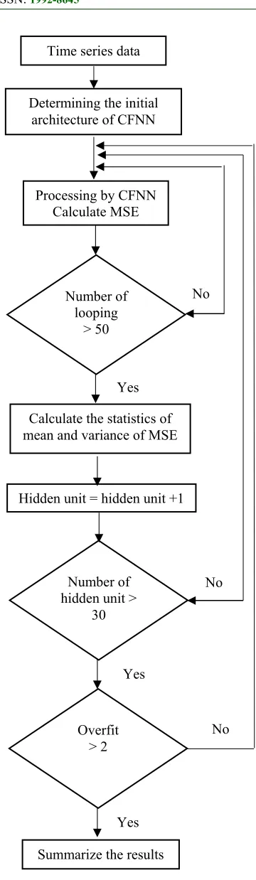
The stages of the proposed procedure are showed in Fig. 2 and described as follows:
1) Determine the lags as input based on the
characteristic of the series
2) for i = 1 to 10 # i = the number of hidden unit
for j = 1 to 30 # j = the number of looping Calculate the MSE
end end
Calculate the mean and variance of MSE
3) Overfit and underfit
4) Back to stage 2
There are two data types observed in this research. The first is the generatied data from Seasonal ARIMA (SARIMA) model and the second is the real case of the ten daily rainfall data from Season Zone 36 of Central Java Province.
3.1 Application in the Data Generated from
Seasonal Model
In this part, we specified the
ARIMA(0,0,1)(0,0,1)12 model with the length of
500. We divide the data into two parts. The 450 first data as training and the 50 remaining as testing. Following the base model, the input candidates used were lags 1, 12 and 13. As the overfit technique we used lags 1-13 as alternatif input, and chosen the best one based on the minimum MSE of the training data. Processing was done with the Levenberg-Marquardt, Conjugate Gradient and BFGS optimization. As with the proposed procedure, in each optimization method and each specified architecture we repeat the process 50 times. The statistics of MSE were resulted and it be used as hint to select the best one. The results shown are the best results of any optimization method for a particular architecture.
Table 1 illustrates the summary of the results. In this case, the network which the 1, 2, 12, 13 lags as input with the Conjugate Gradient optimization method has got well out sample prediction showed by the least mean of out sample MSE. Moreover, this method also yield the most stable result indicated by the minimum variances in both in-sample and out sample prediction. The resulting values are much smaller than two other methods. This condition reinforces the notion that the Conjugate Gradient method is the best choice for the optimization method on the NN model in the specified generated data. Meanwhile, Levenberg-Marquardt method yield the minimum in-sample prediction with the 1-13 lags as input. However, the resulting value does not vary much with the two other methods. Similarly, in almost all inputs tested on the BFGS algorithm, the mean and variance of No
Time series data
Determining the initial architecture of CFNN
Processing by CFNN Calculate MSE
Number of looping
> 50
Calculate the statistics of mean and variance of MSE
No
Yes
Hidden unit = hidden unit +1
Summarize the results Number of hidden unit >
30
Overfit > 2
No
Yes
[image:5.612.89.531.51.705.2]Yes
[image:5.612.94.274.79.698.2]7012 the measured model's accuracy result in a poorer value. Therefore, it can be concluded that Conjugate Gradient optimization is the most
[image:6.612.127.485.157.709.2]recommended method to be chosen for the intended data.
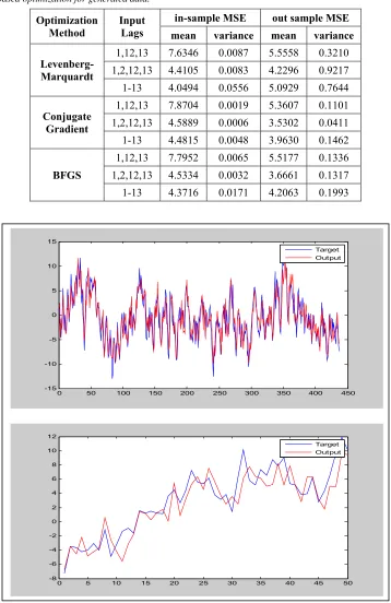
Table 1: Summary of CFNN processing with gradient-based optimization for generated data.
Optimization
Method Input Lags
in-sample MSE out sample MSE
mean variance mean variance
Levenberg-Marquardt
1,12,13 7.6346 0.0087 5.5558 0.3210
1,2,12,13 4.4105 0.0083 4.2296 0.9217
1-13 4.0494 0.0556 5.0929 0.7644
Conjugate Gradient
1,12,13 7.8704 0.0019 5.3607 0.1101
1,2,12,13 4.5889 0.0006 3.5302 0.0411
1-13 4.4815 0.0048 3.9630 0.1462
BFGS
1,12,13 7.7952 0.0065 5.5177 0.1336
1,2,12,13 4.5334 0.0032 3.6661 0.1317
1-13 4.3716 0.0171 4.2063 0.1993
Figure 3: in-sample and out sample prediction and the actual of the simulation data
0 50 100 150 200 250 300 350 400 450
-15 -10 -5 0 5 10 15
Target Output
0 5 10 15 20 25 30 35 40 45 50
-8 -6 -4 -2 0 2 4 6 8 10 12
7013 The goodness of the proposed method also can be seen from the plot in Fig. 3. The plot is the result of running process of CFNN with Conjugate Gradient optimization with 1, 2, 12, 13 lags as input. It can be seen that the prediction (output) result has approached the actual data (target) succesfully. In the in-sample prediction, the prediction has almost come close to its actual perfectly. Whereas, the out sample prediction also still can adhere the actual until many step ahead.
3.2 Application in the Rainfall Data
The data used in this research was the ten-daily rainfall data in ZOM 145 of Jumantono Ngadirojo Wonogiri, province of Central Java, Indonesia from January 2012 to December 2016. The length of data is 180 and it divided into two part, the first 150 data as training and the 30
[image:7.612.103.510.338.554.2]remaining as testing. Based on the plot of the series, it can be determined that the candidates of input are lags of 1, 2 and 18. By the overfitting, the additional inputs are also included. In the first alternative model, the lag of 17 is added and the second alternative, the 1-18 lags are used as input. Table 2 shown the statistics of the processing by CFNN model by using the investigated input and the overfit. As in the simulation data, in this part we applied the proposed procedure with the three gradient-based optimization methods. In each optimization method, the various architectures also have been developed for choosing the best one. The unit hidden is chosen from one to ten to obtain the least mean and variance of the in-sample and out sample prediction. In table 2, the results shown are the best results of any optimization method for a particular architecture.
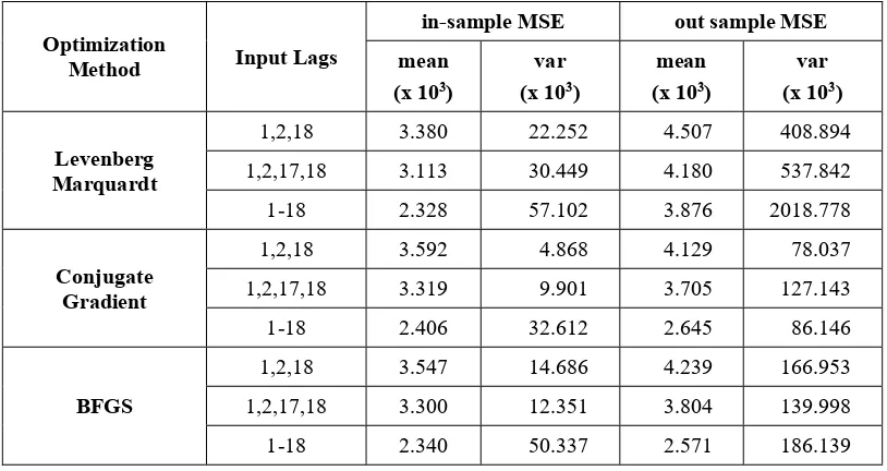
Table 2: Summary of CFNN processing with gradient-based optimization for rainfall data.
Optimization
Method Input Lags
in-sample MSE out sample MSE
mean (x 103)
var (x 103)
mean (x 103)
var (x 103)
Levenberg Marquardt
1,2,18 3.380 22.252 4.507 408.894
1,2,17,18 3.113 30.449 4.180 537.842
1-18 2.328 57.102 3.876 2018.778
Conjugate Gradient
1,2,18 3.592 4.868 4.129 78.037
1,2,17,18 3.319 9.901 3.705 127.143
1-18 2.406 32.612 2.645 86.146
BFGS
1,2,18 3.547 14.686 4.239 166.953
1,2,17,18 3.300 12.351 3.804 139.998
1-18 2.340 50.337 2.571 186.139
The in-sample prediction resulting from the CFNN model at the rainfall data showed the similar results in the three optimization methods with the same archiecture, that is the 1-18 input lags. In each optimization method, this architecture always given the least average of the MSE. The results obtained from the architecture with these inputs have a smaller MSE average than the others. Similarly, the out sample prediction also yield similar results especially for the Conjugate Gradient and BFGS. But, the one important thing for the mean value is the variance. Almost every good average of MSE was followed by the great
7014
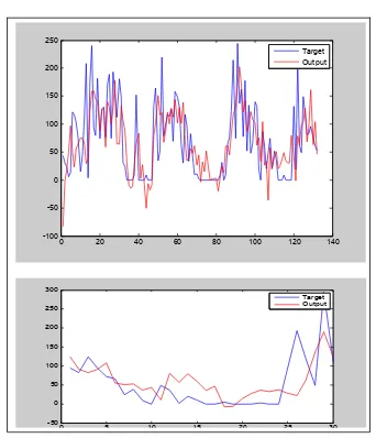
Figure 4: Plot of in-sample and out sample prediction of the rainfall data
Figure 4 is the processing result using the 1,2,18 input lags and the Conjugate Gradient optimization. It can be seen that the prediction (output) has the similar pattern with the actual (target) in both in-sample and out sample data. Generally, the seasonal pattern of the actual series can be followed by the prediction. Many observation points are close to each other with the prediction, some of which coincide. In the out sample prediction, the pattern of the actual data also can be adhered by the output until the end of the series. This reinforces the argument for choosing the architecture.
In this research, the number of hidden unit used is varies from 1 to 10 and each experiment resulting a vary optimal number. It appropriate with Zhang [31] that use the number of hidden nodes
varies from 2 to 14 with an increment of 2. The simulation also given the erratic result. Therefore, Zhang [31] stated that the number of input nodes or the lagged observations used in the neural networks is often a more important factor than the number of hidden nodes. Related to the input, Zhang and Qi [6] stated that neural network has a limited capacity to deal with seasonality in time series, its clearly indicate that neural network are not able to model seasonality directly. Neural network with both detrending and deseasonalize are able to significantly outperform seasonal models in out-of-sample forecasting. Optimization method used in the experiment was Levenberg Marquardt. In this research, we have not done decomposition of data based on its components, either trend or seasonality, but the resulting prediction of CFNN,
0 20 40 60 80 100 120 140
-100 -50 0 50 100 150 200 250
Target Output
0 5 10 15 20 25 30
-50 0 50 100 150 200 250 300
7015 the other class of neural network, has been good enough. It is also interesting to do comparative studies with the separation of its components first. Correspondingly, Curry [12] as the advanced of Zhang and Qi [6], stated that the longer our time series becomes, the more we move to the limits of
the ‘universal approximation’ property.
Multiplicative models combining a time trend and a set of seasonal dummies can be regarded as linear combinations of sinusoidal functions with typical terms t cos(t) and t sin(t), but it still need some theoretical foundation to be established, with a view to supporting empirical studies. As in Zhang and Qi [6], the optimization method used in this research was Levenberg Marquardt, the default of the routine MATLAB toolbox. Curry [12] needs 120 hidden units of FFNN for getting better result, but in the case the network still struggles after a certain point. The interesting result of Curry [12] is that the errors enter towards the end of the series rather than at the beginning. It similar with the result of this research, although with smaller architecture. We can state that generally, there is no guarantee that the bigger architecture gives the better result. However, the comparison between FFNN and CFNN still cannot be concluded and requires a more in-depth study.
In Hedayat [17], the gradient descent method with momentum weight/bias learning rule has been used to train CFNN. The determination of minimum number of necessary hidden units is completely practical. Presently, the best method is making an educated guess. Main criteria selected to adjust the optimal architecture and the training set parameters are the necessary epochs which are needed to reach a desirable mean squared error for learning process, and also average and maximum relative errors for testing data gained after stopping criteria are reached. The simulation studied show that network training with a larger number of hidden units takes more time. Training and testing by a wide variety of learning rates of the gradient descent method to qualify the parameters of the considered CFNN is needed. In Narad [18], the Levenberg Marquardt has been used for optimizing CFNN but applied in other field and type of data. Similar with this research, fast convergence with a few epochs and time were needed for getting the optimal weights.
4. CONCLUSION
In almost previous research, the experiments done are usually only used a single optimization technique. This paper presented a new approach of selecting the network architecture and the best
gradient-based optimization for CFNN model at time series data using the statistics of the model accuracy criteria. The average and variance of the mean square error resulting from repeating process of the CFNN given the goodness illustration of each optimization method. By using this approach, the chosen technique will more appropriate to the type of the series predicted. This is due to the consideration of the stability of predicted results in each experiment, instead of the results of a certain experiment. It will be an interesting open problem if we try to compare with the non-gradient-based optimization techniques.
ACKNOWLEDGEMENT
The authors would like to thank the Rector of Diponegoro University Semarang which has supported and provided research grants of International Scientific Publication Program No. 345-18/UN.5.1/PG/2017.
REFERENCES:
[1] O. Donskikh, D.A. Mikanov, and A.A. Sirota, “Optical Methods of Identifying the Varietes of the Components of Grain Mixtures Based on Using Artificial Neural Networks for Data
Analysis”, Journal of Theoretical and Applied
Information Technology, Vol. 96, No. 2, 2018 [2] T. Nanda, B. Sahoo, H. Beria, and C.
Chatterjee, “A Wavelet-Based Non-Linear
Autoregressive with Exogenous Inputs
(WNARX) Dynamic Neural Network Model for Real-Time Flood Forecasting Using
Satellite-Based Rainfall Products”, Journal of
Hydrology, Vol. 539, 2016, pp. 57–73
[3] Y. Karaca, Case Study on Artificial Neural
Networks and Applications, Applied
Mathematical Sciences, Vol 10, No 45, 2016, pp:2225-37.
[4] Y. Kashyap, A. Bansal, A.K. Sao, Solar radiation Forecasting with Multiple Parameters
Neural Networks, Renewable and Sustainable
Energy Reviews, Vol 49, 2015, pp:825-35 [5] Y. Kashyap, A. Bansal, A.K. Sao, Solar
radiation forecasting Using Neural Networks: a
Modeling Issues, International Journal of
Advanced Information Science and Technology (IJAIST), Vol.3, No.9, September 2014, pp 109-118
[6] J.P. Zhang and M. Qi, “Neural Network Forecasting for Seasonal and Trend Time
Series”, European Journal of Operational
7016 [7] F. Mekanik, M.A. Imteaz, S.G. Trinidad, and A.
Elmahdi, “Multiple Regression and Artificial Neural Network for Long-Term Rainfall Forecasting Using Large Scale Climate Models”, Journal of Hydrology, Vol. 503, 2013, pp. 11–21
[8] M. Nasseri, K. Asghari, M.J. Abedini, “Optimized scenario for rainfall forecasting using genetic algorithm coupled with artificial
neural network”, Expert Systems with
Applications, Vol. 35, 2008, pp. 1415–1421 [9] S. Asadi, J. Shahrabi, P. Abbaszadeh, and S.
Tabanmehr, “A new hybrid artificial neural networks for rainfall–runoff process modeling”, Neurocomputing, Vol. 121, 2013, pp. 470–480 [10] H. K. Cigizoglu, P. Askin, A. Ozturk, A.
Gurbuz, O. Ayhan, M. Yildiz, and İ. Uçar, "Artificial neural network models in
rainfall-runoff modelling of Turkish rivers",
International congress on river basin management, 2007, pp. 560-571
[11] K. Benmahdjouba, Z. Ameura, and M. Boulifa, “Forecasting of Rainfall using Time Delay Neural Network in Tizi-Ouzou (Algeria)”, Energy Procedia, Vol. 36, 2013, pp. 1138 – 1146
[12] B. Curry, “Neural networks and seasonality:
Some technical considerations”, European
Journal of Operational Research, Vol. 179, 2007, pp. 267–274
[13] S.R. Devi, P. Arulmozhivarman, C. Venkatesh and P. Agarwal, “Performance Comparison of Artificial Neural Network Models for Daily
Rainfall Prediction”, International Journal of
Automation and Computing, Vol. 13, No. 5, October 2016, pp. 417-427
[14] N. Kumar, A. Middey, P.S. Rao, “Prediction and examination of seasonal variation of ozone with meteorological parameter through artificial neural network at NEERI, Nagpur, India”, Urban Climate, Vol. 20, 2017, pp. 148-167 [15] O.N.A. Allaf, “Cascade-Forward vs. Function
Fitting Neural Network for Improving Image Quality and Learning Time in Image
Compression System”, Proceedings of the
World Congress on Engineering Vol II WCE 2012, July 4 - 6, 2012, London, U.K.
[16] S. Tengeleng and N. Armand, “Performance of Using Cascade Forward Back Propagation Neural Networks for Estimating Rain Parameters with Rain Drop Size Distribution”, Atmosphere, Vol. 5, 2014, pp. 454-472
[17] A. Hedayat, H. Davilu, A.A. Barfrosh, and S. Sepanloo, “Estimation of research reactor core
parameters using cascade feed forward artificial
neural networks”, Progress in Nuclear Energy,
Vol. 51, 2009, pp. 709–718
[18] S. Narad and P. Chavan, “Cascade Forward Back-propagation Neural Network Based Group Authentication Using (n, n) Secret Sharing Scheme”, Procedia Computer Science, Vol. 78, 2016, pp. 185 – 191
[19] V.K. Patki, S. Shrihari, B. Manu, Water Quality Prediction in Distribution System Using Cascade Feed Forward Neural Network, International Journal of Advanced Technology in Civil Engineering, ISSN: 2231–5721, Volume-2, Issue-1, 2013
[20] G. Capizzi, G.L. Sciuto, P. Monforte, C. Napoli, Cascade feed forward neural network-based model for air pollutants evaluation of single monitoring stations in urban areas, International Journal of Electronics and Telecommunications, Vol 61, No 4, 2015 Dec 1, pp:327-32.
[21] M. Singh, S. Kaur, Weekly WiMAX Traffic Forecasting using Trainable Cascade-Forward Backpropagation Network in Wavelet Domain, International Journal of Application or Innovation in Engineering & Management (IJAIEM), Volume 3, Issue 7, July 2014, pp 197-202
[22] I.M. Yassin, R. Jailani, M. Ali, M.S. Amin, R. Baharom, A. Hassan, A. Huzaifah, Z.I. Rizman, Comparison between cascade forward and multi-layer perceptron neural networks for NARX functional electrical stimulation
(FES)-based muscle model, International Journal on
Advanced Science, Engineering and Information Technology, Vol 7, No 1, 2017, pp :215-21
[23] R. A. Chayjan and M. E. Ashari, Comparison between Artificial Neural Networks and Mathematical Models for Equilibrium Moisture
Content Estimation in Raisin, Agricultural
Engineering International: the CIGR Ejournal. Manuscript 1305. Vol. XII, April, 2010
[24] A. Pwasong and S. Sathasivam, “A new hybrid quadratic regression and cascade forward
backpropagation neural network”,
Neurocomputing, Vol. 182, 2016, pp. 197-209 [25] D.S. Badde, A.K. Gupta, V.K. Patki, Cascade
7017 [26] Mohammad Subhi Al-batah, Umi Kalthum
Ngah, Mutasem Sh. Alkhasawneh, Habibah Hj Lateh, Lea Tien Tay, and Nor Ashidi Mat Isa,
Landslide Occurrence Prediction Using
Trainable Cascade Forward Network and
Multilayer Perceptron, Mathematical Problems
in Engineering, Volume 2015, Article ID
512158, 9 pages
http://dx.doi.org/10.1155/2015/51215 Hindawi Publishing Corporation, 2015
[27] S. Sapna, A. Tamilarasi and M.P. Kumar, “Backpropagation Learning Algorithm Based on Levenberg Marquardt Algorithm”, Computer Science and Information Technology, Vol. 2, 2012, pp. 393-398
[28] Y. Al Bayati, N.A. Sulaiman and G.W. Sadiq, A
“Modified Conjugate Gradient for
Backpropagation Neural Network Algorithm”, Journal of Computer Science, Vol. 5, No. 11, 2009, pp. 846-856
[29] M.S. Apostolopoulou, D.G. Sotiropoulos, I.E. Livieris and P. Pintelas, “A Memoryless BFGS
Neural Network Training Algorithm”, the 7th
IEEE International Conference on Industrial Informatics, 2009, pp. 216-221
[30] E.K.P. Chong, and S.H. Zak, An Introduction to Optimization 2nd edition, Wiley-Interscience Series in Discrete Mathematics and Optimization, John Wiley and Sons, New York, 2001
[31] Zhang, G., 1998. Linear and nonlinear time series forecasting with artificial neural networks. Ph.D. Dissertation, Kent State University, Kent, OH.