5949
TEXTURE RECOGNITION USING CO-OCCURRENCE
MATRIX FEATURES AND NEURAL NETWORK
1SUHAIR H. S. AL-KILIDAR, 2LOAY E. GEORGE
1Baghdad University, College of Science, Department of Mathematical Science, Iraq
2Baghdad University, College of Science, Department of Computer Science, Iraq
E-mail: 1[email protected], 2[email protected]
ABSTRACT
Texture Recognition is used in various pattern recognition applications and classification texture that possess a characteristic appearance. This research paper aims to provide an improved scheme to provide enhanced classification decision with need to increase the procession time significantly. This research studied the discriminating characteristics of textures by extracting them from various texture images using Gray Level Co-occurrence Matrix (GLCM). Three different sets of features are proposed: the first set is a simple modified features extracted from the traditional Gray Level Co-occurrence Matrix (GLCM); the second set uses two sub-sets of features extracted from two GLCM calculated using two displacement values; the third way was passing the extracted set of GLCM through Artificial Neural Network (ANN) for classification purpose. The considered method was applied on 13 classes of textures belong to three sets from Salzburg Texture Image Database (i.e., bark, marble and woven fabric), each set holds 16 images per class, so the total 208 image images were tested. Each image was separated into four bands of color component (i.e., red, green, blue, and gray). So, the analysis work was done for 56 different set of characteristics (14 features per band). Then calculating the average and standard deviation and finally conducting scatter analysis for each feature to find out the best discriminating features which can be used for attaining best classification. The experiments showed that the results are competitive, the test results indicated that the attained average accuracy of classification is improved up to (99.71%) for the training set and (99.3 %) for the testing set.
Keywords: Texture Recognition, characteristics, Co-occurrence Matrix (GLCM) features, Artificial Neural Network (ANN), Features extraction.
1. INTRODUCTION
Texture is the term used to characterize the surface of a given object or region, and it is one of the main features utilized in image processing and pattern recognition; it refers to the appearance, structure and arrangement of the parts of an object within the image. Although one can intuitively associate several image properties such as smoothness, coarseness, depth, regularity etc. with texture [14]. Image textures may be complex visual patterns composed of entities or regions with sub-patterns with the characteristics of brightness, color, shape, size, etc. Texture can be regarded as a similarity grouping in an image [31]. Some of texture definitions are perceptually motivated, and others are driven completely by the application in which the definition will be used. [11] has compiled a catalogue of texture definitions in the computer vision literature.
5950 strips had extracted the statistical textural features using co-occurrence matrix presented by Haralick and also calculated the geometrical features to handles the problem of classification of the defect types and he proposed SVM (Support Vector Machine). Khan et at. [17] have proposed an automatic brain tumor detection that can detect and localize brain tumor in Magnetic Resonance Imaging (MRI). The proposed method works in two stages: the first stage is used to extract the features from images using Grey level Co-occurrence matrix; while in the second stage the extracted features are used as input for Support Vector machine (SVM). Antony et at. [3] introduced an automated system to assess a patient's risk of Melanoma, which is the dangerous form of skin cancer, using images of their skin lesions captured using a standard digital camera. The features are extracted using Gray Level Co-occurrence Matrix (GLCM). Then the features are compared with the given database for classification using Artificial Neural Network (ANN). The attained experiment results reflected high accuracy compared to other tested algorithms.
The new scheme high lights the possibility of increasing the classification accuracy using the same set of features by with difference system parameters. Where this paper answers the question about improving the classification performance using a combined set of features derive for co-occurrence Matrix concept, presents enhanced methods for texture identification using Spatial Gray Level Co-occurrence matrices GLCM. These methods could improve system recognition accuracy since they depend on combinations of Spatial Gray Level Co-occurrence matrices (GLCMs), and consequently, the combinations of their corresponding derived features. Also, the classification results in case of using ANN classifier methods instead of Euclidean distance criteria are given.
The next sections are organized as follows. In the next section, an overview of texture analysis methods used in this research is presented by clarifying some of the concepts related to the used methods and the attributes that can be derived from them. Section 3 explains the adopted methodology in this search and the proposed manners for modifying of the traditional method and the applied combination between the GLCMS derived from two parameter of displacement vector. In fourth section the attained results are presented and compared
with results of some published articles. Finally, in the last section, the main conclusions are presented.
2. OVERVIEW
One of the most common category of features to characterize texture falls into statistical approach; for example it analyzes the spatial distribution of color bands values that is one of the defining qualities of texture. Depending on the number of pixels defining the local features can be used as discriminating attributes. Statistical methods can be classified into first order (one pixel), second order (relation of two pixels), and higher order (three or more pixels) [29]. First order statistics are estimated using the behavior of each pixel value without considering the neighborhood relations; i.e., ignoring the spatial interaction between image pixels. The Second- and higher order statistics are estimating the properties of two or more pixel values occurring at specific locations relative to each other.
2.1 Spatial Gray-Level Co-Occurrence Matrices (GLCM):
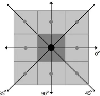
The Spatial Gray -Level Co-occurrence Matrix (GLCM) was introduced by [15], it estimates the image properties related to second-order statistics. C(i,j) is defined by first specifying a displacement vector d = (Δx, Δy) and analyzing all possible pairs of pixels, placed apart by the separated fixed distance d; typically, d takes small values. Assume the considered pairs of pixels having gray levels i and j and arranged in a given direction, θ (i.e., four pixel alignment directions are normally considered (0◦, 45◦, 90◦, and 135◦), see Figure1. Then, different distances between the pairs of pixels were considered. C(d,θ) is of size G×G, where G is the number of gray levels possible to be encoded in an
image. Each element of co-occurrence matrix, ci,j (i,
j = 0...G−1), represents a probability of occurrence of a pair of pixels with gray levels of i and j, for the first and for the second pixel, respectively.
5951
homogeneity), Correlation (measures linear
dependency of gray levels on neighboring pixels) and Variance (Sum of Squares).
[image:3.612.105.280.262.431.2]Other features can be calculated from the sums of probabilities that related to specified intensity sums or differences [4]. Some of features derived from such vectors are: Sum Average, Sum Variance, Sum Entropy, Difference Average, Difference Variance, and Difference Entropy.[7] proposed two additional GLCM-based features that measure the skewness (the lack of symmetry) of the matrix C(d,θ): Cluster Shade, Cluster Prominence.
Figure 1: The four directions of adjacency defined for calculation of Haralick texture features. The Haralick statistics are calculated for co-occurrence matrices generated using each of these directions of adjacency
2.2 Neural Network
Artificial Neural Networks (ANNs) are nonlinear mapping structures based on the biological neuron system. They used to simplify the problems of prediction or classification, as a powerful tool for modelling especially when the underlying data relationship is unknown. ANNs can recognize and learn correlated patterns between input data sets. In this research the selected features that succeeded in classifying during the scattering analysis tests were
used with the corresponding target values (i.e., number of classes) for training and testing the
adopted feed forward AAN. They are parallel computational models included of densely interconnected adaptive processing units, therefore ANNs became the focus of much attention, largely because of their ease treat complicated problems and their used in wide range of applicability. ANN computational model formed from several single
units (called artificial neurons); they connected with coefficients (weights) which constitute the neural structure, they known as Processing Elements (PE) in processing information. Each (PE) has a weighted input, transfer function and one output. The learning methods in neural network can be classified into three basic types (i) supervised learning (ii) unsupervised learning and (iii) reinforced learning. There are several types of architecture of neural network, the one most widely used are the feed forward networks; they allow signals to travel one way only; from input to output. There is no feedback (loops); that is the output of any layer does not affect that same layer. They are extensively used in pattern recognition [24].
3. MATERIALS AND METHODS
3.1 Data Description
5952 3.2 Methodology
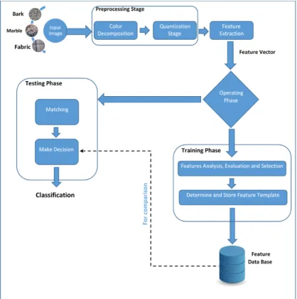
This section presents the implemented steps and design considerations of the introduced recognition system. Figure (2) presents the overall design of the proposed recognition system; it is consist of the following stages:
Prep-processing stage.
Features vector extraction stage.
[image:4.612.90.299.236.446.2] Classification stage.
Figure 2: General Diagram of the Proposed System
3.2.1 Prep-processing stage
The first stage in any recognition system is pre-processing. In this stage, a sequence of image processing operations is applied to make the image (that loaded to the system as input) appropriate for extracting the related information to get the best discrimination results. In this research the following pre-processing steps were applied:
A. Read images and color decomposition As a first step of this work, the loaded images are decomposed into the four color bands (or channels). The basic color components are Red, Green, Blue and the 4th considered band is the Brightness (i.e., Gray)), this gray color value is calculated by the
equation:
That is, the color image component are separated into four dedicated channels red, green and blue and their corresponding brightness, such that each channel is assigned as only one color component.
B. Quantization
The quantization process overcomes the main drawback in using Co-occurrence Matrices which is a large memory requirement for storing these matrices and usually resulting high computational complexity. The quantization process removes some of the information details through mapping a group of close data values to a single value; in other words mapping each pixel value of each band matrix from the range (0 to 255) to a new value (0 to MaxBandVal):
The quantization was applied on the four considered color bands of each image. In this study different MaxBandVal values (8, 16, 20, 24, 28, 32, 40 and 55) were tested to find the optimal value that leads to best discrimination performance. The results indicated that the value MaxBandVal =32 led to highest classification results.
3.2.2 Feature extraction stage
After passing through the previous steps (read image and color decomposition and quantization by one gray level), the feature extraction stage is performed to extract some of textural attributes. The purpose of the feature extraction is to obtain a set of texture measures that can be used to discriminate among different texture pattern classes. Many different feature extraction methods have been introduced over the past few decades and they used for texture classification problems as described previously [2, 5, 21, 28, and 35]. In this paper, one of the most important texture analysis methods is used to extract a certain kind of feature vector by utilizing the spatial gray level co-occurrence matrices. Also, some variants for this method are introduced to develop more efficient sets of discriminating features.
A. Apply spatial gray level co-occurrence method
5953 computed from each determined spatial co-occurrence matrices of each color band; the set of features consists of energy, entropy, contrast,
homogeneity, autocorrelation, coarseness,
directionality and etc. They are determined using the following equations:
Where P(i,j) is the probability of C(i,j)
Where µi, µj, σi and σj are the mean and Std.
Where x and y are the coordinates (row and column) of an entry in the co-occurrence matrix and Px+y is the
probability of co-occurrence matrix coordinates summing to x+y.
….. (16)
Where , HX, HY are
entropies of Px and Py,
,
and
B. Application of modified methods
B1. The first variant of the gray level co-occurrence matrices
Three additional GLCM matrices were added in addition to the four gray level co-occurrence matrices. The traditional GLCM are established for the four directions (0◦, 45◦, 90◦, and 135◦), and the additional three matrices are calculated as: (i) mean of the corresponding elements traditional GLCM matrices; (2) the maximum values of the corresponding elements of the four traditional GLCM; and (3) the Minimum values of the corresponding elements. So, seven matrices are generated for calculating the feature attributed from these 7 GLCM instead of four traditional Matrices using the abovementioned features equations.
Because the choice of the displacement vector d is an important parameter in the definition of the gray-level co-occurrence matrix. Occasionally, the co-occurrence matrix is computed for several values of d and the one which leads to highest classification result is adopted. In this work different distance values (d) were tested (i.e., 1, 5, and 10). It was noticed that the best attained results is when the choice d=1 is adopted.
B2. Combined feature vector using two GLCM each belong to different displacement value In the second carried out method two values of the displacement value (d) were applied to construct two GLCM matrices from them a combined feature vector is constructed. The combined feature vector consists of 28 characteristics (i.e., 14 extracted from each GLCM). The conducted tests showed that the best pair of displacement values is {d1=1, d2=10} they led to highest classification results. Another combined feature vector was considered it is the integration of a couple of GLCM features sets; each set belongs to certain quantization value (i.e., MaxBandValue); the attained highest classification score was not so encouraging enough in comparison with the results of other two methods.
3.2.3 Features analysis
5954 attributes was accomplished due to their inter-class stability. Through the training phase, features were selected from the overall set of features; and the selection was due to the comprehensive tests which were conducted on the training set of samples to find out the best set of features that can be used to yield highest matching score.
3.2.4 Classification stage
A. Matching
The matching steps compute the match score (or in other words, the similarity degree) between the features vectors extracted from the input samples with the stored templates. The similarity score should be high for samples which belong to the same class and low for those belong to different classes. Sample matching is usually a difficult pattern recognition task due to large intra-class variations (i.e., variations in sample images for the same class) and large inter-class similarity (i.e., similarity between samples images from different class). In our project, the features which have been extracted in previous stage, have been used either to match the tested samples data that previously stored in database (i.e., belong to training set) or other samples (i.e., testing set). To perform matching, the features of the samples belong to training set are used to yield the template mean feature vector for each class. The mean feature vector (̅F) of each class, and the corresponding standard deviation vector (σ) are determined saved in a dedicated database during training phase, these parameters are used as template vectors. The determined using the following equations:
Where c, f, s are the classes number, feature number and sample number, respectively.
While in matching stage their similarity degrees are computed with the feature vector extracted from the tested samples. The similarity distance measure for tested feature (f) is computed by used the feature value determined from the tested sample and the corresponding feature mean value and standard division (determined for each class). The most commonly used similarity measure is Euclidean
distance measure (D1), but, the main weakness of
the basic Euclidean distance function is that if one of input features has a relatively large range, then it can overpower the effectiveness of other features. The considered matching problem here is dynamic; that is every feature may not have similar behaviors like others. So, another type of similarity distance
measures (like: D2, D3 and D4) were computed. The
results of using these four distance measures were
compared and noticed that the results of measure D1
are always better than others' results; so the
normalized Euclidean distance (D4) had been used
to evaluate the similarity degree between the extracted feature vectors of the tested samples (fj)
and the templates representing the classes [10]:
Where is the template (mean) of class i, and is the standard deviation of class i.
In order to maximize the probability of the match classification and minimize misclassification rate. The efficiency of classification is calculated for each distance using the following equation [5]:
B. Enhance success or recognition rate
Incremental comprehensive tests were conducted on the data set for combination of two features using the same previous matching criteria to find out the best set of features that can be used to yield best matching rates. Thus a partial set consisting of 30 pairs of combined traits have been chosen from the comprehensive set of attributes (i.e. as total there are 784 features).
5955 It was observed during the repeated additions some of the features were repeated many times.
C. Using Artificial Neural Network (ANN) The set of training feature vectors was used to train the established ANN; these vectors are extracted from images and saved in feature vector database. The training vectors are used to train a feed forward neural network by adjusting its nodes weights and bias values using back-propagation algorithm. The computed weights and bias values of trained network are, also, registered in the dedicated database. Before feeding the feature vector to the network the value of the involved features must normalized because it is important to unify the dynamic ranges of all involved features. The normalization of feature (f) was performed using the following equation:
Where FNorm(fi) is the normalized value of ith
feature, fi is the value of ith feature, µfi is the mean
of it, and σfi is its standard deviation.
In the training stage the network starts with a random set of weights and the training sample is presented at the input layer. Then, the outputs of the network are evaluated and compared with the expected "binary" output vector, the error is calculated and the results were fed back from output layer to adjust weights. These steps are repeated for all training set, and at each time the weights are adjusted. The training continues until one of the stopping conditions is satisfied (i.e., the number of iterations is passed over or the overall error becomes lower than a predefined target error) and the network is considered ready for decision making tasks.
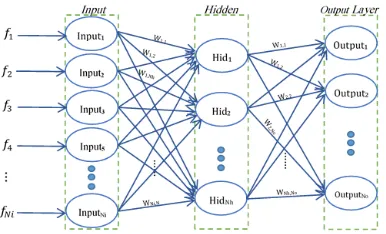
[image:7.612.322.515.106.223.2]In the established system, the three layers feed forward neural network architecture had been adopted. The adopted neural network consists of one input layer, one output layer, and one hidden layer, see Figure 3. The number of input nodes is set equal to the number of the best combination of discriminating features. the number of hidden nodes was varied to find out the best smallest number of hidden nodes required to get best recognition; taking into consideration that each additional hidden node causes extra computation during both training and classification phases.
Figure 3: The structure of Feed Forward Neural Network
4. EXPERIMENT RESULTS
A part of Salzburg Texture Image Database (STex) was employed for classification evaluation. Some of these samples are presented (see Figure 4). At first made detail comparisons between various features of the traditional method (GLCM) was conducted, and the attained test results indicated that the best average accuracy of classification is (81.2%). While, the best results obtained from applying the introduced enhanced methods reached around (99.71%) for the training set and (99.3%) for the testing set (see Table 2).
[image:7.612.313.523.507.648.2]5956
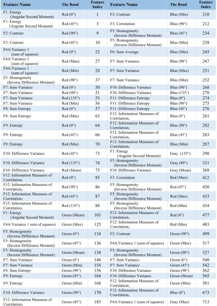
Table 1: Feature Index Table for Gray Level Co-occurrence Matrices
Feature Name The Band Feature Index Feature Name The Band Feature Index
F1: Energy
(Angular Second Moment) Red (0°) 1 F2: Contrast Blue (Min) 210 F1: Energy
(Angular Second Moment) Red (45°) 3 F3: Correlation Blue (90°) 212 F2: Contrast Red (90°) 9 F5: Homogeneity (Inverse Difference Moment) Blue (45°) 234
F2: Contrast Red (45°) 10 F5: Homogeneity (Inverse Difference Moment) Blue (Min) 238 F4A:Variance 1
(sum of squares) Red (0°) 22 F6: Sum Average Blue (Min) 245 F4A:Variance 1
(sum of squares) Red (Max) 27 F7: Sum Variance Blue (90°) 247 F4A:Variance 1
(sum of squares) Red (Min) 28 F7: Sum Variance Blue (Max) 251 F5: Homogeneity
(Inverse Difference Moment) Red (90°) 37 F7: Sum Variance Blue (Min) 252 F7: Sum Variance Red (0°) 50 F10: Difference Variance Blue (90°) 268 F7: Sum Variance Red (90°) 51 F10: Difference Variance Blue (135°) 270 F7: Sum Variance Red (135°) 53 F11: Difference Entropy Blue (0°) 274 F7: Sum Variance Red (Min) 56 F11: Difference Entropy Blue (90°) 275 F8: Sum Entropy Red (0°) 57 F11: Difference Entropy Blue (45°) 276
F8: Sum Entropy Red (Min) 63 F12: Information Measures of Correlation
1 Blue (0°) 281
F9: Entropy Red (0°) 64 F12: Information Measures of Correlation
1 Blue (90°) 282
F9: Entropy Red (45°) 66 F12: Information Measures of Correlation
1 Blue (45°) 283
F9: Entropy Red (Min) 70 F12: Information Measures of Correlation
1 Blue (Min) 287
F10: Difference Variance Red (45°) 73 F1: Energy (Angular Second Moment) Gray (135°) 298
F10: Difference Variance Red (135°) 74 F5: Homogeneity (Inverse Difference Moment) Gray (90°) 331
F10: Difference Variance Red (Mean) 75 F10: Difference Variance Gray (Mean) 369 F12: Information Measures of
Correlation1 Red (0°) 85 F3: Correlation Red (Max) 412
F12: Information Measures of
Correlation1 Red (90°) 86
F5: Homogeneity
(Inverse Difference Moment) Red (45°) 430 F12: Information Measures of
Correlation1 Red (45°) 87
F5: Homogeneity
(Inverse Difference Moment) Red (Max) 433 F12: Information Measures of
Correlation1 Red (135°) 88
F5: Homogeneity
(Inverse Difference Moment) Red (Min) 434 F1: Energy
(Angular Second Moment) Green (Mean) 103
F12: Information Measures of
Correlation1 Red (0°) 477
F4A:Variance 1 sum of squares) Green (Max) 125 F12: Information Measures of Correlation
1 Red (Min) 483
F5: Homogeneity
(Inverse Difference Moment) Green (0°) 134 F2: Contrast Green (90°) 499 F5: Homogeneity
(Inverse Difference Moment) Green (45°) 136 F4A:Variance 1 (sum of squares) Green (Max) 517 F5: Homogeneity
(Inverse Difference Moment) Green (Mean) 138
F5: Homogeneity
(Inverse Difference Moment) Green (90°) 527 F7: Sum Variance Green (0°) 148 F7: Sum Variance Green (0°) 540 F7: Sum Variance Green (Min) 154 F7: Sum Variance Green (45°) 542 F8: Sum Entropy Green (90°) 156 F10: Difference Variance Green (90°) 562 F9: Entropy Green (45°) 164 F10: Difference Variance Green (Mean) 565
F9: Entropy Green (Min) 168 F12: Information Measures of Correlation
1 Green (Min) 581
F10: Difference Variance Green (90°) 170 F12: Information Measures of Correlation
1 Blue (0°) 673
F12: Information Measures of
5957
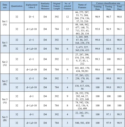
Table 2: The best selected GLCM features which provided highest recognition rate
Where (A) denoted to (11 samples for training & 5 samples for testing) in each class, (B) denoted to (8 samples for training & 8 samples for testing) in each class.
Data
sets Quantization
displacement value d
Similarity Distance Measures
Original Feature Length
No. of selected Features
Name of Features
Correct classification rate Training
Data
Testing Data
Total Data
Set 1 (A)
32 D =1 D4 392 12
66, 275, 287, 53, 73, 268, 268, 274, 136,
37, 53, 210
90.9 90.7 90.8
32 d=1,d=10 D4 784 12
88, 168, 562, 477, 148, 75, 713, 331, 63, 483, 20, 134
95.8 96.9 96.1
Set 1 (B)
32 d =1 D4 392 9
3, 245, 369, 87, 86, 247,
164, 238, 276 99.0 82.6 90.8
32 d=1,d=10 D4 784 6 565,156, 433 3, 673, 527, 99.0 84.6 91.8
Set 2 (A)
32 d =1 D4 392 11
27, 287, 298, 154, 234, 185,
9, 37, 85, 1, 212
99.3 100 99.5
32 d=1,d=10 D4 784 6 103, 483, 170, 434, 50,281 98.6 100 99.0
Set 2 (B)
32 d =1 D4 392 7
57, 283, 125, 238, 170, 10,
28 100 99.0 99.5
32 d=1,d=10 D4 784 4 138, 517, 434, 56 100 99.0 99.5
Set 3 (A)
32 d=1 D4 392 9 28, 252, 270, 282, 64, 27, 51, 125, 148
100 100 100
32 d=1,d=10 D4 784 8
74, 542, 126, 412, 136, 9,
134, 499 100 100 100
Set 3 (B)
32 d=1 D4 392 4 22, 282, 251, 70 100 97.1 98.5
32 d=1,d=10 D4 784 3 540, 581, 430 100 97.9 98.9
Deciding the proper number of nodes in the hidden layer is a very important part of deciding the overall
neural network architecture. Trial-and-error
mechanism was adopted in this research work to find out the proper number of hidden nodes.
5958
Table 3: The Effect of "Number of Hidden Nodes" on Classification Accuracy Rate
Data Sets
No. of Hidden Nodes
displacement value d =1 No. of Hidden
Nodes
displacement value d=1, d=10
Min Training
Error Accuracy Rate Classification Min Training Error Accuracy Rate Classification
Set 1 (Bark)
11 0.080386 96.1 8 0.076091 97.5
16 0.072829 98.5 13 0.041506 98.0
21 0.069756 98.5 18 0.069837 98.5
22 0.103319 97.5 20 0.042184 99.5
26 0.042834 99.0 22 0.020463 100
28 0.053527 98.0 29 0.025862 100
Set 2 (Marble)
8 0.154744 91.8 10 0.297521 82.6
12 0.143583 93.7 14 0.150265 92.7
17 0.140797 94.7 19 0.280568 84.1
19 0.099444 96.1 33 0.233978 87.0
Set 3 (Fabric)
11 0.057102 98.0 15 0.137369 97.5
28 0.038145 98.5 17 0.089333 97.5
29 0.094947 98.0 33 0.197876 98.5
40 0.031542 98.5 49 0.045835 98.5
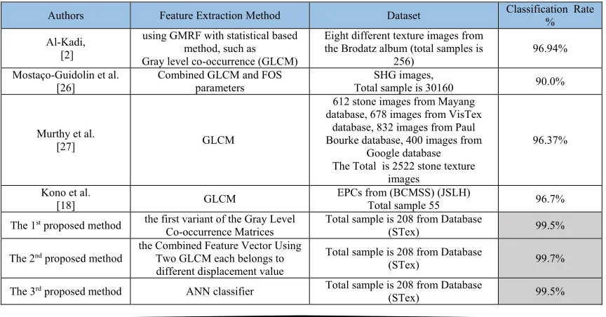
5. COMPARISON WITH PREVIOUS STUDIES
Many research work to try to distinguish textures using different methods performed in the recent years. As a result of the lack of research using the same dataset, the comparison will be compared with research that using the same features extracted from GLCM , Table 4 classify the results of the recently published works that are made on independent recognition systems, tested on different dataset by using Co-occurrence Matrices. The results shows the effectiveness of proposed methods.
Table 4: comparison of recognition rate with recently published work using GLCM
Authors Feature Extraction Method Dataset Classification Rate %
Al-Kadi, [2]
using GMRF with statistical based method, such as Gray level co-occurrence (GLCM)
Eight different texture images from the Brodatz album (total samples is
256)
96.94%
Mostaço-Guidolin et al. [26]
Combined GLCM and FOS parameters
SHG images,
Total sample is 30160 90.0%
Murthy et al.
[27] GLCM
612 stone images from Mayang database, 678 images from VisTex
database, 832 images from Paul Bourke database, 400 images from
Google database The Total is 2522 stone texture
images
96.37%
Kono et al.
[18] GLCM
EPCs from (BCMSS) (JSLH)
Total sample 55 96.7%
The 1st proposed method the first variant of the Gray Level
Co-occurrence Matrices
Total sample is 208 from Database
(STex) 99.5%
The 2nd proposed method the Combined Feature Vector Using Two GLCM each belongs to
different displacement value
Total sample is 208 from Database
(STex) 99.7%
The 3rd proposed method ANN classifier Total sample is 208 from Database
[image:10.612.91.523.517.743.2]5959 6. CONCLUSIONS
In this paper, two modified GLCM methods are introduced; these methods are improved variants to the traditional Co-occurrence Matrices (COM). The introduced methods was applied on texture image such that each belong to certain class, with need to handily the problems occurred due to overlapping and shadowing. The best recognition rates of the proposed method was (%99.5) for classification accuracy rate when using the first variant of the Gray Level Co-occurrence Matrices, While when using the Combined Feature Vector Using Two GLCM each belongs to different displacement value; the best attained recognition rate had reached (%100) for classification accuracy rate. The attained rates are better than those reached in the traditional method; when the system used ANN for recognition decision instead of using the traditional statistical approach the best recognition rates of the proposed system was (%100) for recognition accuracy rate.
REFRENCES
:
[1] Abbadeni, N.; "Computational
Perceptual Features for Texture
Representation and Retrieva". IEEE Transactions on Image Processing, Vol. 20, Issue 1, January-2011. Pp. 236 – 246.
[2] Al-Kadi, O.S., "Combined Statistical
and Model Based Texture Features for Improved Image Classification". In: 4th International Conference on Advances in Medical, Signal & Information Processing. Santa Margherita Ligrue, Italy, 2008.
[3] Antony, A., Ramesh, A., Sojan, A.,
Mathews, B., & Varghese, M. T. A.; "Skin Cancer Detection Using Artificial
Neural Networking". International
Journal of Innovative Research in Electrical, Electronics, Instrumentation and Control Engineering Vol. 4, Issue 4, April-2016.
[4] Bankman, I.N.; "Handbook of Medical
Image Processing and Analysis". Edited by Second Edition. Academic Press, 2002.
[5] Bhiwani, R.J., Khan, M.A., Agrawal,
S.M.; "Texture Based Pattern
Classification", International Journal of Computer Applications, Vol. 1, No. 1, 2010. Pp. 54-56.
[6] Chu, A., Sehgal,C.M. and Greenleaf,
J.F.; "Use of Gray Value Distribution of Run Lengths for Texture Analysis"; Vol. 12, in Pattern Recognition, by Lett. June 1990.Pp. 415–420.
[7] Coggins, J.M.; "A Framework for
Texture Analysis Based on Spatial Filtering"; East Lansing, Michigan:
Ph.D. Thesis, Computer Science
Department, Michigan State University East Lansing, Michigan, 1983.
[8] Commowick, O., Lenglet, C., and
Louchet, C.; "Wavelet Based Texture Classification and Retrieval", Ecole Normale Superieure de Cachan, 2003. Pp. 1-20.
[9] Conners, R.W., Mcmillin, C.W., Lin, K.,
& Vasquez-Espinosa, R.E.; "Identifying and Locating Surface Defects in Wood: Part of an Automated Lumber Processing System", IEEE Transactions on Pattern Analysis and Machine Intelligence, Vol. PAMI-5, No. 6; 1983. Pp. 573-583.
[10] Conners, R.W., Harlow, C.A.; "Toward a Structural Textural Analyzer Based on Statistical Methods". Comput. Vision Graph, Vol. 12, Pp. 224-256, 1980. [11] Coggins, J. M.; "A Framework for
Texture Analysis Based on Spatial Filtering". Ph.D. Thesis, Computer Science Department, Michigan State University East Lansing, Michigan, 1982.
[12] Duda, D. "Texture Analysis as a Tool for Medical Decision Support. Part 1: Recent Applications For Cancer Early Detection". Advances in Computer Science Research, Atlantes Press. Vol. 11, 2014. Pp. 61-84
[13] Galloway, M.M.; "Texture Analysis Using Gray Level Run Lengths", Vol.2, June-1975. Pp. 429-441
5960 [15] Haralick, R.M., Shanmugam, K.S., and
Dinstein I; "Textural Features for Image Classification", IEEE Trans. Syst., Man, Cybern., Vols. SMC-3, 1973, Pp. 610– 621.
[16] Jernigan, M.E. and D'Astous, F.; "Entropy-Based Texture Analysis in the Spatial Frequency Domain", IEEE Trans. Pattern Anal. Machine Intell., Vols. PAMI-6, March-1984. Pp. 237– 243.
[17] Khan, A., Syed, N.A., Reyaz, M.; "Image Processing Techniques for Brain Tumor Extraction from MRI Images using SVM Classifier". International Journal on Recent and Innovation
Trends in Computing and
Communication, ISSN: 2321-8169, Vol. 3 , Issue 5, 2015 Pp. 2707- 2711. [18] Kono, K., Hayata, R., Murakami, S.,
Yamamoto, M., Kuroki, M., Nanato, K., Takahashi, k., Miwa, k., Tsutsumi, y., Okada, K., Mikami, T., Masauzi, N., & Kaga, S.. Quantitative Distinction of the
Morphological characteristic of
Erythrocyte Precursor Cells with Texture Analysis Using Gray Level Co‐occurrence Matrix. Journal of Clinical Laboratory Analysis (JCLA), 2017, Pp. 1-6.
[19] Kwatra, V., Sch dl, A. , Essa, I.A., Turk, G., and Bobick, A.F.; "Graphcut Textures: Image and Video Synthesis Using Graph Cuts, SIGGRAPH 2003: In ACM Transactions on Graphics, Vol. 22, July-2003 Pp. 277-286.
[20] Laine, A., and Fan, J.; "Texture Classification by Wavelet Packet Signatures", IEEE Trans. Pattern Anal. Machine Intell.. Vol. 15, November-1993, Pp. 86–1191.
[21] Ling, L., Ming, L., & YuMing, L.;
"Texture Classification and
Segmentation Based on Bidimensional Empirical Mode Decomposition and
Fractal Dimension", Education
Technology and Computer Science, ETCS '09, the 1st International Workshop on (IEEE), Vol l., 2009, Pp. 574-5772, March-.
[22] Liu, S. and Jernigan, M. E.; "Texture Analysis and Discrimination in Additive Noise", Comput. Vis., Graph., Image
Process., Vol. 49, 1990, Pp. 52–67. [23] Nixon, M.S., Aguado, A.S.; "Feature
Extraction and Image Processing", Edition no. 1, edited by a member of the
Reed Elsevier group, Oxford
Publication, 2002.
[24] Michie D., Spiegelhalter, D.J., Taylor, C.C.; "Machine Learning, Neural and Statistical Classification", First Edition, Cambridge CB2 2SR, U.K, 1994. [25] Mohamad, A.R.; "Design of Online
Classifier for Surface Defect Detection and Classification of Cold Rolled Steel Coil", MTech Thesis, Department of
Electrical Engineering, National
Institute of Technology, Rourkela 2013. [26] Mostaço-Guidolin, L. B., Ko, A. C. T., Wang, F., Xiang, B., Hewko, M., Tian, G., ... & Sowa, M. G. . "Collagen Morphology and Texture Analysis: from Statistics to Classification". 2013. Scientific Reports, 3.
[27] Murthy, G. S. N., & Veerraju, T.; "A Novel Approach Based on Decreased Dimension and Reduced Gray Level Range Matrix Features for Stone Texture Classification". International Journal of Electrical and Computer Engineering (IJECE), Vol. 7(5). 2017. Pp. 2502-2513.
[28] Nurzynska, K., Kubo, M., and Muramoto, K.; "Grey Scale Texture
Classification Method Comparison
Considering Object and Lighting Rotation", International Journal of Computer Theory and Engineering, Vol. 5, No. 1, February 2013, Pp. 19-23,. [29] Ojala, T., & Pietikäinen, M.; "Texture
Classification, Machine Vision and Media Processing Unit", University of Oulu, Finland, Available at.
http://homepages.inf.ed.ac.uk/rbf/CVonl ine/LOCAL_COPIES/OJALA1/ texclas.htm, Junuary 2004.
[30] Patil, S., Udupi, V.R.; "A Computer
Aided Diagnostic System for
5961 [31] Rosenfeld, A., & Dwyer, S.J.; "Digital
Pic. Analysis", Springer-Verlag, New York, 1976.
[32] Schistad, A.H. and Jain, A.K.; "Texture Analysis in the Presence of Speckle Noise". IEEE Geoscience and Remote Sensing Symposium, Houston, Texas, USA, 1992.
[33] Schmid, C.; "Constructing Models for
Content-Based Image Retrieval",
Proceedings of the IEEE Conference on
Computer Vision and Pattern
Recognition, Kauai, Hawaii, USA, 2001.
[34] Sheha, M.A., Mabrouk, M.S., & Sharawy, A.; "Automatic Detection of Melanoma Skin Cancer Using Texture Analysis", International Journal of Computer Applications, Vol. 42, No. 20, 2012, Pp. 22-26,.
[35] Tou, J.Y.; Tay, Y.H.; and Lau, P.Y.;
"Recent Trends in Texture
Classification: A Review", Symposium
on Progress in Information &
Communication Technology, Kuala Lumpur, Malaysia, 17th to 18th, Dec, 2009.
[36] Unser, M., and Eden, M.;