Price, R.J. and Crawford, Ian and Barlow, M.J. and Howarth, I.D. (2001) An
ultra-high-resolution study of the interstellar medium towards Orion. Monthly
Notices of the Royal Astronomical Society 328 (2), pp. 555-582. ISSN
0035-8711.
Downloaded from:
Usage Guidelines:
Please refer to usage guidelines at
or alternatively
An ultra-high-resolution study of the interstellar medium towards Orion
R. J. Price,
PI. A. Crawford, M. J. Barlow and I. D. Howarth
Department of Physics and Astronomy, University College London, Gower Street, London WC1E 6BT
Accepted 2001 August 6. Received 2001 August 6; in original form 2001 May 18
A B S T R A C T
We report ultra-high-resolution observationsðR<9105Þof NaI, CaII, KI, CH and CH1 for interstellar sightlines towards 12 bright stars in Orion. These data enable the detection of many more absorption components than previously recognized, providing a more accurate perspective on the absorbing medium. This is especially so for the line of sight to the Orion nebula, a region not previously studied at very high resolution. Model fits have been constructed for the absorption-line profiles, providing estimates for the column density, velocity dispersion and central velocity for each constituent velocity component. A comparison between the absorption occurring in sightlines with small angular separations has been used, along with comparisons with other studies, to estimate the line-of-sight velocity structures. Comparisons with earlier studies have also revealed temporal variability in the absorption-line profile of
z
Ori, highlighting the presence of small-scale spatial structure in the interstellar medium on scales of <10 au. Where absorption from both Na0and K0 is observed for a particular cloud, a comparison of the velocity dispersions measured for each of these species provides rigorous limits on both the kinetic temperature and turbulent velocity prevailing in each cloud. Our results indicate the turbulent motions to be subsonic in each case. Na0/Ca1abundance ratios are derived for individual clouds, providing an indication of their physical state.Key words:line: profiles – ISM: atoms.
1 I N T R O D U C T I O N
The Orion region is well known for its ongoing star formation. The most active sites of star formation may be found on the western faces of the giant molecular clouds (GMCs) that form the backdrop of the constellation. In the model of the Orion region proposed by Cowie, Songaila & York (1979), the Orion OB1 association is located on the western side of the molecular-cloud complex, centred around the point where the Orion A and B GMCs meet. Using observations of CO, Bally et al. (1990) find the molecular gas located nearest to the centre of the association to exhibit the most positive radial velocities. These features are considered to be a result of shocks and ionizing radiation from association stars (Bally et al. 1990).
It is the influence of the association stars that is considered to produce the many loops and shell structures visible in this direction. In the model for the region proposed by Cowie et al. (1979), Barnard’s Loop, which has the form of an incomplete
elliptical ring centred on the OB1 association [not enclosing thel
Orionis association (Pickering 1890; Barnard 1895)], is interpreted
as being an HIIregion at the inner edge of a dense shell of
swept-up material. This is considered to be a part of the much larger
Orion – Eridanus superbubble (Reynolds & Ogden 1979; Brown, Hartmann & Burton 1995; Heiles et al. 1999). Exterior to Barnard’s Loop, Cowie et al. (1979) suggest the presence of a
fast-moving (100 km s21), low-density shell centred on the Orion OB1
association, denoted ‘Orion’s cloak’ because of the way in which it appears to cover the Hunter’s back.
While the constellation’s youngest stars reside beneath the surface of the molecular clouds, the youngest subgroup (Id;
,0:5106yr old; Warren & Hesser 1978) is present very near the
surface, producing the Great Nebula in Orion (M42, NGC 1976,
Orion A). The oldest of the stellar subgroups (Ia;<8106yr old;
Warren & Hesser 1978) is located at the greatest distance from the parent molecular cloud.
The apparent brightness of the stars in Orion aids the spectroscopic study of the intervening interstellar (IS) matter. It
was an investigation into the spectrum and orbit of d Ori by
Hartmann (1904) that led to the first identification of absorption arising in the interstellar medium (ISM). Subsequent observations
of the H and K lines of CaIIby Beals (1936) revealed double and
asymmetric components in the spectra of Orion stars, the first evidence pointing to the existence of multiple discrete IS clouds. These were the first steps in the study of a very complex IS sightline.
Earlier high-resolution surveys of matter in the ISM (e.g. Hobbs
P
E-mail: [email protected]
1969a, hereafter H69; Hobbs 1969b,c, 1978b; Marschall & Hobbs 1972; Hobbs & Welty 1991; Welty, Hobbs & Kulkarni 1994, hereafter W94; Welty, Morton & Hobbs 1996, hereafter W96; Welty & Hobbs 2001, hereafter W01; detailed further in Section 4)
have included observations of stars in the direction of Orion;
however, none have concentrated on the ISM in this direction. The work of O’Dell et al. (1993, hereafter OD93), while focusing on the
inner Orion nebula, utilized lower-resolutionðR<9104ÞCaIIK
observations of the four Trapezium stars, and earlier NaID2
observations of Hobbs (1978b).
The aims of the current project are to obtain absorption-line profiles for the brighter Orion stars using spectra acquired with the Ultra-High-Resolution Facility (UHRF) at the Anglo-Australian
Telescope. The resolving power of these data ðR<9105Þ
exceeds all known previous observations of this region. Observations at such high spectral resolution enable many of the blended lines seen towards complex regions such as the Orion nebula (M42) to be resolved for the first time. These absorption components are then used to investigate the velocity structure of the Orion region, and the intervening ISM. Comparisons of
absorption components found independently for CaII, NaIand KI
have been made in order to identify individual IS clouds producing recognizable absorption in one or more of these species. Where observations of closely spaced sightlines are available (i.e., the
M42 region and l Ori association), comparisons are also made
between sightlines. This enables the identification of absorption systems, where absorption from individual IS clouds may be seen
in more than one sightline. Where both NaI and KI line
components are observed for a particular cloud, rigorous limits on
both the kinetic temperature (Tk) and line-of-sight
root-mean-square (rms) turbulent velocity (vt) are derived (Section 5).
Following the identification of temporal variability in the IS
absorption profile ofdOrionis (Price, Crawford & Barlow 2000,
hereafter Paper I; Price, Crawford & Howarth 2001, hereafter Paper II), we compare current observations with those presented in previous studies, in order to identify any temporal variability present in other sightlines (Section 4).
2 O B S E R VAT I O N S
The observations reported here were obtained using the UHRF on the 3.9-m Anglo-Australian Telescope. The majority of the observations were obtained during 1994 (January 20–23, and December 16–18 inclusive), with further observations made in 1996 (December 2), 1999 (January 29 and July 31) and 2000 (March 15). During 1994 January, a Thomson charge-coupled
device (CCD) ð10241024, 19-mm pixels) was used, while in
1999 January, the MITLL2 CCDð40962048, 15-mm pixels) was
used. The remaining observations used a Tektronix CCD
ð10241024, 24-mm pixels). In all, 12 stars in Orion have been
observed, including four in the M42 region. Table 1 lists the stars observed and relevant properties.
The spectrograph was operated with a confocal image slicer (Diego 1993), and the CCD output was binned (by factors of 4 or 8) perpendicular to the dispersion direction in order to reduce the readout noise. The instrument was operated in its highest resolution mode, providing a velocity resolution (as measured from the observed width of a stabilized He – Ne laser line) of
0:34^0:01 km s21 full width at half-maximum (FWHM) ðR¼
880 000Þfor all observations. Other aspects of the instrument and
observing procedures have been described in detail by Diego et al.
(1995) and Barlow et al. (1995). Table
1. Ste llar da ta, an d a summ ary of UHRF exposure s made for the tar gets observ ed in thi s study . Stella r posi tions ha v e been obtained from Hof fleit & Ja schek (1982 ). W here av ailable, V mag nitudes and dis tances ha v e been obt ained from the H ippar cos an d Ty ch o catalo gues (ESA 1997 ). In the cases of u 1Ori A and C an d u 2Ori A, dis tances are not av ailable fro m the Hipp ar cos catalo gue and ha v e been taken fro m G oudis (1982 ). Spectra l typ es ha v e gene rally been obt ained fro m Mor gan, Code & Whitford (1955 ); in the case of l Ori and u 1 Ori A, Co nti & Alsch uler (1971 ) and Hofflei t & Jaschek (1982 ), res pecti v ely , ha v e been used. Deri v ations of E ð B 2 V Þ ha v e been made using the tab ulat ions of Deuts chma n, D av is & Schild (1976), and da ta fro m Hofflei t & Jaschek (1982 ; u 1Ori A and C) and the Hipp ar cos and Ty ch o catalo gues (ESA 1997; all other stars). Stella r he liocentric rad ial v elocitie s ( v( ) ha v e bee n obta ined from W ilson (1953 ) and Ev ans (1967 ). Columns 10–1 4 sho w the tota l ex posu re times in se conds , follo we d by the number of ind ividua l ex posu res, in pa renthes es; in the case of d Ori, this only repres ents the 1994 obser v ati ons. Star HD lb V Sp. type E ð B 2 V Þ Dist. v( T otal ex posu re (s ) ( 8 0)( 8 0) (pc) (km s 2 1 )C a II KN a I D1 K I l 7698 CH l 4300 CH 1 l 4233 12 3 4 5 6 7 8 9 1 0 1 1 1 2 1 3 1 4 b O ri 34085 209 14 2 25 15 0.28 B8 Ia 2 0.01 237 1 56 2 38 20.7 ^ 0.9 2200 (3) 3600 (4) 200(1 ) – – d O ri 36486 203 52 2 17 44 2.20 O9.5II 0.11 281 1 85 2 53 16.0 ^ 2.0 1200 (1) 3600 (3) – – – f 1Ori 36822 195 24 2 12 17 4.38 B0 IV 0.16 302 1 92 2 57 33.2 ^ 0.9 2400 (2) 1800 (1) – – 1200( 1) l Ori 36861 195 03 2 12 00 3.52 O 8III 0.16 324 1 109 2 66 33.4 ^ 0.5 2800 (3) 1200 (1) – – 1800( 2) u 1Ori A 37020 209 01 2 19 23 4.98 O7 0.34 < 450 33.4 ^ 2.0 5400 (3) – – – – u 1 Ori C 37022 209 01 2 19 23 5.13 O6 0.35 < 450 28.0 ^ 5.0 5400 (4) 2400 (2) – 3600( 2) 2400( 2) u 2Ori A 37041 209 03 2 19 22 4.98 O9.5V 0.22 < 450 35.6 ^ 2.0 3600 (2) 2250 (1) – 3600( 2) 1200( 1) i Ori 37043 209 31 2 19 35 2.74 O 9III 0.10 407 1 185 2 97 21.5 ^ 0.9 3600 (2) 3600 (3) – – – e Ori 37128 205 13 2 17 14 1.69 B0 Ia 0.07 412 1 246 2 113 25.9 ^ 0.9 3000 (3) 2000 (2) 2400 (2) – – s O ri 37468 206 49 2 17 20 3.77 O9.5V 0.13 352 1 166 2 85 29.1 ^ 2.0 3600 (2) 1200 (2) – – – z Ori 37742 206 27 2 16 35 1.70 O9.5Ib 0.07 251 1 62 2 42 18.1 ^ 0.9 3000 (3) 3000 (3) 2400 (2) – – k Ori 38771 214 31 2 18 30 2.04 B0.5Ia 0.06 221 1 46 2 32 20.5 ^ 2.0 – 2400 (2) 2400 (2) – –
The spectra were extracted from the individual CCD images
using theFIGAROdata reduction package (Shortridge et al. 1999) at
the UCL Starlink node. Scattered light and CCD dark current levels were measured from the inter-order region and subtracted. Wavelength calibration was performed using a Th – Ar lamp. An
indication of the accuracy of this process for the NaI and CaII
regions may be obtained from the comparison of radial velocities of clouds producing well-determined absorption in both of these
species (e.g., the detection of both NaID1and CaIIK absorption,
at velocities of 2:90^0:01 and 2:88^0:01 km s21, respectively,
towardseOri). Furthermore, comparison of these data with previous
studies has, in general, shown excellent agreement. However, in the case of six stars for which observations are presented here and in
the NaI survey of W94, a small systematic velocity offset of
<20:30^0:1 km s21is detected in the W94 data.
In the case of the KI l7699 data, only two Th – Ar lines were
found to occupy the spectral range of our observations, thus limiting our ability to calibrate wavelengths accurately for these
data. A comparison of corresponding NaI and KI absorption
components indicates there to be a velocity shift<20:3 km s21
present in the KIspectra; however, the velocity shift is not constant
over the spectral range. This has not been allowed for in the following analysis.
Continuum normalization has been achieved by division with low-order polynomial fits to the continuum; however, in the case of
bOri, the presence of strong stellar CaII absorption has created
some uncertainty with this procedure, resulting in the use of a manually drawn continuum. A typical spectral range of
<130 km s21was obtained, which in general is centred on the IS
absorption. In the case of the CaIIobservations ofu1
Ori A and C
andu2Ori A, a lack of well-determined red-wing continuum does
lead to some uncertainty in the normalization process; however, the requirement of only first- and second-order polynomial fits to the (blue) continuum alleviates this uncertainty. Removal of telluric
(water) lines from the NaIand KI spectra has been achieved by
division by atmospheric template spectra, observed towards the
bright, lightly reddened staraVir [note thataVir actually exhibits
a single weak NaI absorption component at a velocity of
211.2 km s21(Welsh, Vedder & Vallerga 1990), but this is clear of
all absorption components observed towards the stars in this study]. These atmospheric templates were acquired with the same
instrument during observing runs in 1994 (NaI) and 1993 (KI). To
account for small variations in the strengths of the atmospheric lines between the different spectra, the optical depth of the adopted atmospheric template was scaled before division. The spectra were converted to a heliocentric velocity frame and individual exposures of the same star/transition were added (the number of individual observations comprising each spectrum is shown in parentheses after the total exposure times in Table 1). All velocities referred to here are heliocentric unless otherwise stated.
During the analysis of the data, a small discrepancy in the zero
level was found in the cores of saturated NaID1lines towardsl
and f1
Ori. The lines were seen to reach 0.01 and 0.02 of the continuum, respectively; therefore the zero level of the two spectra were readjusted. This provides a guide to the likely uncertainty in
the zero level of the remaining (uncorrected) NaI spectra. Since
fully saturated interstellar CaIIK lines have never been observed, it
is not possible to assess the zero-level error for the CaIIregion in
this manner; however, the excellent agreement seen between these observations and those presented in other studies (see Section 4)
suggests zero-level errors in the CaIIregion to be minor (i.e. of the
order 1–2 per cent).
3 L I N E - P R O F I L E A N A LY S I S
The absorption lines were initially modelled using the IS line
fitting routines in theDIPSO spectral analysis program (Howarth,
Murray & Mills 1993). These models were subsequently optimized
through the use of theVAPIDline fitting routine (Howarth et al. in
preparation), which evaluates the set of component parameters that produce the minimum rms residuals. During the fitting procedure, all component parameters were unconstrained. The number of components employed in each model was kept to a minimum, such that any additional components did not provide a significant
statistical improvement to the fit (with the exception of the KI
model ofkOri, discussed in Section 5.4). In a small number of
cases this has resulted in the inclusion of very broad components which, statistically, cannot be replaced by multiple, narrower
components (zOri CaII,v(¼23:74;sOri CaII,v(¼10:25;l
Ori NaI, v(¼30:74Þ. Nevertheless, we feel that the use of
unconstrained model parameters is preferable since, although the
CaII, NaIand KImodels have been independently generated, the
generally good agreement between the CaII, NaI and KI
absorption model components suggests that the majority of the individual clouds have been identified. Furthermore, it has been possible to model simultaneously the various spectra for a given
star. Where a cloud is identified in both NaIand CaII, its velocity
can be constrained to be equal in both species, but remain variable to optimize the fit. Simultaneous absorption models were generated for a selection of stars but show little, if any, variation with those
generated independently. In fact, our results show that Ca1 is
generally present in warmer regions of the cloud than Na0,
therefore providing no reason to force the CaIIand NaIabsorption
to occur at exactly the same velocity. In the case of Na0and K0
where there are good reasons to assume the species to be co-spatial, and therefore to model them simultaneously, the variable velocity
offset detected in the KIspectra (Section 2) makes the procedure
impracticable.
By reconstructing the absorption models presented in the high-resolution, high-S/N (signal-to-noise ratio) surveys conducted by
W94 (NaI), W96 (CaII) and W01 (KI), it becomes possible to
compare their exact component structures with those now derived
here. In the case of CaIIwe find that, with the exception ofu1
Ori C, towards which we identify significant additional structure,
the higher S/N achieved by W96 in their CaIIobservations has in
general allowed the use of a greater number of components. In a small number of cases, our use of fully unconstrained parameters in the modelling process has led to the inclusion of very broad
components (zOri,v(¼23:74;sOri,v(¼10:25Þnot seen in the
W96 models. In general, very good agreement is present between
the NaI component structures modelled here and by W94. The
higher resolution employed by us typically enables additional substructure to be resolved, while the higher S/N that we have achieved allows us to identify additional weak components. In the
case of the KIobservations, there is good agreement between the
column densities found here and those of W01. The higher S/N
achieved by W01 in their KIobservation ofeOri makes possible
the detection of a weak component at a velocity of 17.17 km s21
(corresponding to our cloud 8 towards this star). The higher
resolution employed here has, in the case ofzOri, resolved three
additional components, while for k Ori, further substructure is
suggested in the spectrum and, although not statistically
significant, has been modelled on the grounds of our NaI
observations (see Section 5.4).
The atomic data adopted for the various transitions are listed in
Table 2. The resulting line-profile parameters, heliocentric radial
velocity, v(, velocity dispersion,b, and column density, N, are
listed in Table 3, along with the 1s, single-parameter errors. In the
case of NaIand KI,v(corresponds to the weighted mean velocity
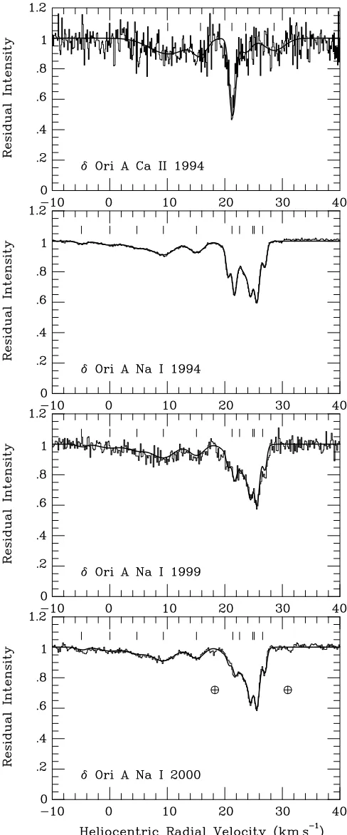
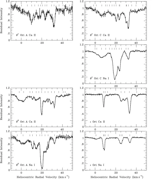
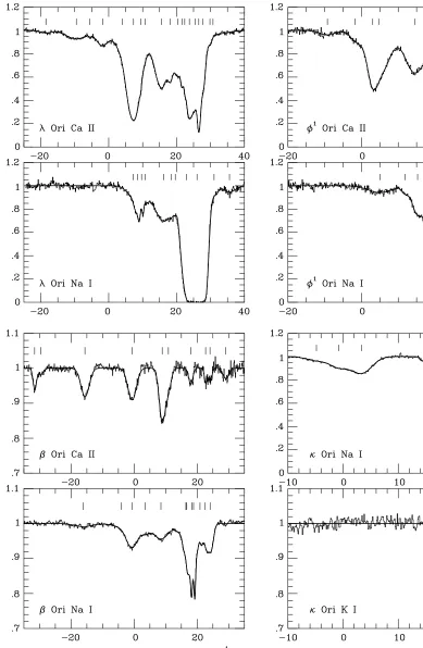
of the two hyperfine split (HFS; discussed further below) components. The corresponding best-fitting model profiles, after convolution with the instrumental response function, are shown in Fig. 1, overplotted on the observed line profiles.
The hyperfine splitting of the NaID1 and KI l7699 lines
(amounting to a separation of 1.08 km s21, or 21 mA˚ , in the case of
NaID1; and to 0.35 km s21, or 9 mA˚ , in the case of KIl7699) has
been accounted for in the modelling of these transitions (see Table 2). The ability of the UHRF to resolve distinctly the HFS of
narrow (and not strongly blended) NaID1 components places
rigorous limits on the range of permittedbvalues. Furthermore, the
UHRF is capable of resolving intrinsic linewidths for components
with b values as low as 0.2 km s21 (which, in the case of Na,
corresponds to a cloud with Tk¼50 K, and vt¼0:05 km s21Þ.
Many examples of resolved HFS components are visible in Fig. 1, a
notable example being the 2.90 km s21 component observed
towards e Ori, which has a derived b value of 0.35 km s21
(discussed in Section 5). However, even at the resolution employed here we still find regions of closely blended components that cannot be unambiguously disentangled. Indeed, many components present in regions of velocity space containing significant amounts of substructure may remain unidentified, irrespective of the resolution employed.
Where observations of more than one atom/ion are available for
a given star, the comparison of absorptioncomponentspresent in
each waveband enables the identification of individual ISclouds
(numbered according to radial velocity in Table 3). Furthermore, where observations of stars with small angular separations are
available, it is possible to identify absorption systems, whereby
individual IS clouds produce absorption (characterized by components with similar parameters) in more than one sightline.
The identification of these absorption systems will be made in
Sections 7.1 (for the M42 region) and 7.2 (for the l Ori
association). The absorption systems are numbered according to
velocity, but during the discussion of Sections 7.1 and 7.2 the
systemswill be referred to by either an M orl(denoting M42 andl
Ori regions respectively) followed by a bold number, so as to reduce confusion with individual clouds.
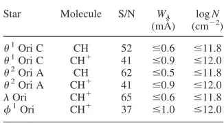
Observations of CHl4300 and/or CH1l4233 have been made
towards a number of our targets; however, no absorption
components have been positively identified in any of these spectra.
Table 4 lists the S/N and upper limits to the equivalent widths (Wl)
and column density of any absorption present in each of these spectra. In general, these values represent better limits than those determined in previous studies (e.g. Hobbs 1973; Federman 1982; Lambert & Danks 1986).
4 S E A R C H F O R T E M P O R A L VA R I A B I L I T Y
Previous observations of IS absorption towards the stars observed here have been made at a variety of resolutions, and include the studies by H69, Marschall & Hobbs (1972), OD93, W94, W96 and W01. The resolving power achieved by the UHRF exceeds that of
these earlier observations, although the NaI survey of W94 did
employ a comparable resolving power ðR¼6105Þ, while the
W96 CaII survey (conducted mainly with a resolving power of
R¼2:5105Þ included two UHRF observations of stars also
observed here. H69 estimated the resolving power of the PEPSIOS
Fabry – Perot interferometer to be approximately 6105, although
a comparison between PEPSIOS and UHRF observations (Barlow et al. 1995) suggested that the resolving power of the former was
probably in the range R<ð1–2Þ 105. For the purposes of
comparison, we here assume a value of R¼2105 for the
PEPSIOS data.
Following the discovery of temporal variability in the IS spectra
ofdOrionis (Papers I and II), an examination of the remaining
spectra has been made in order to identify any variability in other sightlines. Comparisons have primarily been made with the studies by OD93, W94, W96 and W01, for which absorption models have been published, while additional comparisons have also been made with the observations by H69 and Marschall & Hobbs (1972).
However, the presence of telluric absorption in the NaIspectra by
H69 limits our ability to identify confidently temporal variability. By reconstructing the relevant absorption models presented by OD93, W94, W96 and W01, it became easier to compare their observations with ours.
During these comparisons the resolution of our observations was degraded (through Gaussian convolution) to a level equal to that of the observations with which the comparison was being made. In this way, we hope that any changes found cannot be ascribed to the different resolving powers employed. Several examples of possible variability have been found. These are displayed in Fig. 2 and are discussed individually below. Similar investigations carried out by W94 and W96 found no evidence for temporal variability; however, the success of our investigation is primarily due to the availability of the observations made by W94 and W96. In hindsight, subtle variations can also be seen between the observations by W94 and by H69, and between those of W96 and Marschall & Hobbs (1972). The small discrepancy in velocity scales found between our data and those of W94 (noted in Section 2) has been allowed for through the application of small velocity shifts to the W94 data, in order to achieve maximum agreement between data sets.
4.1 dOrionis
Striking line-profile variations have been detected towardsdOri A,
attributed to the passage of an IS cloud, most likely present within
the expanding HI shell surrounding the Orion – Eridanus
super-bubble. The line-profile variability seen towardsdOri A is discussed
in detail in Papers I and II. In the latter paper, absorption-line
[image:5.594.94.236.145.234.2]profile differences betweendOri A anddOri C are also reported,
Table 2. Wavelengths (l) and correspond-ing oscillator strengths (f) adopted for the line-profile analyses. Hyperfine splitting of the NaID1 and KIl7699 transitions has been accounted for in the modelling process. The information is taken from: (1) Morton (1991); (2) Black & van Dishoeck (1988); and (3) Lambert & Danks (1986).
Line l(A˚ ) f Ref.
CaIIK 3933.663 0.635 (1) NaID1 5895.9108 0.119 (1) 5895.9321 0.199 (1) KI 7698.969 0.127 (1) 7698.978 0.212 (1) CH R2(1) 4300.313 0.0051 (2) CH1R(0) 4232.548 0.0055 (3)
T able 3. Co mponent par ameters de ri v ed from the absorpt ion-line mo delling for the Orion stars. F or each v eloci ty com ponent, v alues of v( (he liocent ric rad ial v eloci ty), b (v elocity dispersio n) and N (column densi ty) are sho w n in colu mns 2–4 (for Ca +), 6–8 (for N a 0) an d 9–11 (for K 0). A chie v ed S/N ratio s and total equi v alent w idths ( W l ) are display ed alon gside each star’ s iden tifier . In the case of both Na I and K I absorpt ion, central v elociti es are w ith res pect to the weighted mean of the two hyper fine split com ponen ts. Where Ca II and/ or Na I and/or K I com ponen ts (to wards a gi v en star) appear in the same ro w , and are he nce iden tified by the sa me cloud numbe r (co lumn 1) , the absorptio n is consider ed to occur in the same indi vidual inte rstellar clou d. Co lumn 5 gi v es clou d Na 0/ Ca 1 ratios. Where mult iple entries are mad e with a single clou d number (to wards a gi v en star), absor ption is conside red to arise in multip le unresol v ed clouds and an av erage Na 0/ Ca 1 ratio is obtained fro m the summ ed Na 0an d Ca +column densi ties. Where a N a I componen t posses ses no Ca II count erpart, a 2 s upper limit to the undet ected Ca + colu mn de nsity is deri v ed (see Section 6) and a lo we r limi t to the Na 0/ Ca 1 ratio is obt ained; in the re v ers e situat ion, an upper limit is obta ined. Systems under going possibl e temporal v aria bility (discusse d in Section 4) are iden tified in column 1 wit h a super script ‘†’. In the case of d Ori, also see P apers I and II. Ca II KN a I D1 K I l 7699 Star/ v( b log N Na 0 Ca 1 v( b log Nv ( b log N clou d (km s 2 1) (km s 2 1) (cm 2 2) (km s 2 1) (km s 2 1) (cm 2 2) (km s 2 1) (km s 2 1) (cm 2 2) 1 2 34 5 6 78 9 1 0 1 1 e Ori S = N ¼ 114 ; W l ¼ 85.4 ^ 0.3 mA ˚ S = N ¼ 192 ; Wl ¼ 156.6 ^ 0.1 mA ˚ S = N ¼ 127 ; Wl ¼ 2.7 ^ 0.3 mA ˚ 1 1.17 ^ 0.82 3.47 ^ 0.62 10.84 ^ 0.13 , 0.04 2 2.88 ^ 0.01 0.31 ^ 0.02 10.61 ^ 0.02 1.78 2.90 ^ 0.01 0.35 ^ 0.01 10.8 6 ^ 0.02 3 4.82 ^ 0.13 2.02 ^ 0.37 10.87 ^ 0.14 1.78 4.76 ^ 0.29 2.89 ^ 0.22 11.1 2 ^ 0.04 4a 7.90 ^ 0.21 1.06 ^ 0.30 10.49 ^ 0.19 2.29 9.61 ^ 0.47 2.03 ^ 0.61 11.1 0 ^ 0.18 4b 9.19 ^ 0.08 0.60 ^ 0.14 10.37 ^ 0.27 5 10.8 8 ^ 0.02 0.86 ^ 0.13 11.09 ^ 0.21 2.63 10.9 4 ^ 0.01 0.63 ^ 0.02 11.5 1 ^ 0.03 10.5 5 ^ 0.04 0.54 ^ 0.07 9.87 ^ 0.04 6 12.4 1 ^ 0.02 0.36 ^ 0.07 10.33 ^ 0.13 6.76 12.3 5 ^ 0.02 0.75 ^ 0.04 11.1 6 ^ 0.05 7a 12.5 0 ^ 0.97 2.24 ^ 0.92 11.15 ^ 0.28 0.54 13.6 7 ^ 0.04 0.17 ^ 0.10 9.86 ^ 0.11 7b 14.7 4 ^ 0.02 0.59 ^ 0.03 10.8 4 ^ 0.02 8 17.2 6 ^ 0.03 0.59 ^ 0.06 10.41 ^ 0.07 5.62 17.1 8 ^ 0.01 0.47 ^ 0.01 11.1 6 ^ 0.02 9 18.3 1 ^ 0.19 2.50 ^ 0.24 11.06 ^ 0.05 0.81 17.4 9 ^ 0.07 1.50 ^ 0.09 10.9 7 ^ 0.04 10a 23.8 4 ^ 0.71 1.65 ^ 0.48 10.85 ^ 0.26 3.09 22.7 0 ^ 0.02 0.70 ^ 0.03 11.1 7 ^ 0.01 10b 23.7 9 ^ 0.02 0.35 ^ 0.03 10.8 6 ^ 0.06 11 25.0 7 ^ 0.04 0.87 ^ 0.12 11.06 ^ 0.16 4.57 24.7 7 ^ 0.01 0.58 ^ 0.02 11.7 2 ^ 0.02 24.7 0 ^ 0.04 0.56 ^ 0.07 9.87 ^ 0.04 12 26.2 2 ^ 0.08 0.53 ^ 0.10 10.40 ^ 0.15 9.55 26.0 1 ^ 0.05 0.93 ^ 0.07 11.3 8 ^ 0.04 13 28.0 1 ^ 0.02 1.36 ^ 0.03 11.36 ^ 0.01 0.41 28.1 7 ^ 0.05 0.81 ^ 0.06 10.9 7 ^ 0.04 14 . 11.7 5 29.8 9 ^ 0.20 0.91 ^ 0.24 10.3 9 ^ 0.10 15 37.0 5 ^ 0.26 3.69 ^ 0.37 10.48 ^ 0.04 , 0.09 z Ori S = N ¼ 111 ; W l ¼ 79.7 ^ 0.3 mA ˚ S = N ¼ 156 ; Wl ¼ 150.7 ^ 0.3 mA ˚ S = N ¼ 116 ; Wl ¼ 5.0 ^ 0.2 mA ˚ 1 2 8.56 ^ 0.39 1.84 ^ 0.37 10.29 ^ 0.12 , 0.11 2a 2 5.05 ^ 0.14 1.75 ^ 0.17 11.09 ^ 0.08 1.40 2 6.05 ^ 0.07 0.69 ^ 0.11 10.3 2 ^ 0.07 2b 2 1.85 ^ 0.16 2.07 ^ 0.46 11.12 ^ 0.15 2 3.05 ^ 0.06 0.44 ^ 0.11 10.1 3 ^ 0.14 2c 1.85 ^ 0.88 2.33 ^ 1.51 10.62 ^ 0.37 2 2.23 ^ 0.06 3.43 ^ 0.10 11.4 3 ^ 0.01 2d 2 2.06 ^ 0.03 0.26 ^ 0.07 10.2 2 ^ 0.06 2e† 2 1.07 ^ 0.01 0.44 ^ 0.02 10.9 8 ^ 0.02 2 1.31 ^ 0.06 0.04 ^ 0.42 9.31 ^ 0.13 3a 6.27 ^ 0.37 1.92 ^ 0.93 10.43 ^ 0.29 0.76 8.27 ^ 1.17 2.51 ^ 0.58 10.8 2 ^ 0.38 3b 9.88 ^ 0.18 1.84 ^ 0.48 10.78 ^ 0.16 4 11.4 3 ^ 0.06 0.38 ^ 0.14 9.70 ^ 0.19 4.27 11.5 0 ^ 0.02 0.38 ^ 0.04 10.3 3 ^ 0.06 5 13.7 0 ^ 0.22 2.36 ^ 0.52 10.89 ^ 0.13 1.29 11.6 3 ^ 1.05 2.76 ^ 0.65 11.0 0 ^ 0.26 6† 18.3 9 ^ 0.22 0.95 ^ 0.16 10.68 ^ 0.26 0.96 18.1 1 ^ 0.03 0.62 ^ 0.05 10.6 6 ^ 0.05 7a 19.9 8 ^ 0.51 1.17 ^ 0.80 10.52 ^ 0.34 1.48 19.4 6 ^ 0.19 1.98 ^ 0.20 10.8 3 ^ 0.04 7b 21.5 5 ^ 0.08 0.52 ^ 0.17 10.10 ^ 0.32 8a 23.0 6 ^ 0.05 0.84 ^ 0.05 11.17 ^ 0.08 6.03 22.9 7 ^ 0.01 0.32 ^ 0.02 11.1 9 ^ 0.06 22.9 7 ^ 0.04 0.44 ^ 0.06 10.13 ^ 0.04
T able 3 – cont inued Ca II KN a I D1 K I l 7699 Star/ v( b log N Na 0 Ca 1 v( b log Nv ( b log N cloud (k m s 2 1) (km s 2 1) (cm 2 2) (km s 2 1) (km s 2 1) (cm 2 2) (km s 2 1) (km s 2 1) (cm 2 2) 1 2 34 5 6 78 9 1 0 1 1 8b 23.19 ^ 0.01 0.82 ^ 0.02 11.8 7 ^ 0.01 23.8 0 ^ 0.16 0.16 ^ 0.39 9.20 ^ 0.30 9 23.74 ^ 1.61 5.69 ^ 0.88 11.1 0 ^ 0.18 , 0.03 10 24.59 ^ 0.20 1.21 ^ 0.30 10.9 6 ^ 0.13 1.51 25.08 ^ 0.03 0.51 ^ 0.04 11.1 4 ^ 0.06 11a 26.35 ^ 0.01 0.52 ^ 0.02 10.7 7 ^ 0.04 11.4 8 26.20 ^ 0.01 0.24 ^ 0.03 11.0 9 ^ 0.05 25.7 1 ^ 2.01 0.58 ^ 0.94 9.60 ^ 1.86 11b 26.41 ^ 0.03 0.76 ^ 0.02 11.7 4 ^ 0.02 26.2 4 ^ 0.13 0.31 ^ 0.32 9.94 ^ 0.84 12 37.00 ^ 0.09 1.96 ^ 0.12 10.4 5 ^ 0.02 , 0.08
1994 dOri
S = N ¼ 14 ; Wl ¼ 36.1 ^ 2.0 mA ˚ S = N ¼ 185 ; W l ¼ 60.8 ^ 0.2 mA ˚ 1 . 0.45 2 4.92 ^ 0.12 0.83 ^ 0.23 9.86 ^ 0.06 2 . 0.85 0.03 ^ 0.34 2.44 ^ 0.46 10.3 7 ^ 0.08 3 . 1.29 4.72 ^ 0.20 2.12 ^ 0.43 10.5 2 ^ 0.11 4 10.07 ^ 1.05 7.63 ^ 1.31 11.3 1 ^ 0.07 0.45 9.32 ^ 0.12 2.63 ^ 0.18 10.9 6 ^ 0.03 5 15.77 ^ 0.31 1.26 ^ 0.57 10.5 0 ^ 0.22 1.51 15.07 ^ 0.04 1.56 ^ 0.07 10.6 8 ^ 0.01 6† 21.23 ^ 0.05 0.74 ^ 0.07 11.0 7 ^ 0.04 0.74 21.25 ^ 0.01 0.45 ^ 0.01 10.9 4 ^ 0.02 7a 23.63 ^ 0.25 1.13 ^ 0.42 10.5 9 ^ 0.13 7.08 22.56 ^ 0.53 2.41 ^ 0.33 11.1 2 ^ 0.11 7b 24.85 ^ 0.07 1.38 ^ 0.15 11.1 6 ^ 0.10 8 . 5.13 25.11 ^ 0.01 0.36 ^ 0.02 10.7 4 ^ 0.04 9 . 3.16 26.57 ^ 0.01 0.38 ^ 0.03 10.5 4 ^ 0.04 10 28.56 ^ 0.48 2.59 ^ 0.74 10.7 9 ^ 0.10 , 0.04
1999 dOri
S = N ¼ 31 ; W l ¼ 60.3 ^ 1.4 mA ˚ 6† 21.26 ^ 0.07 0.44 ^ 0.09 10.6 0 ^ 0.05
2000 dOri
S = N ¼ 82 ; W l ¼ 52.1 ^ 0.7 mA ˚ 6† 21.39 ^ 0.05 0.39 ^ 0.06 10.2 4 ^ 0.04 s Ori S = N ¼ 43 ; Wl ¼ 91.0 ^ 1.0 mA ˚ S = N ¼ 114 ; W l ¼ 154. 7 ^ 0.5 mA ˚ 1 2 10.85 ^ 0.27 3.45 ^ 0.40 10.7 5 ^ 0.04 , 0.07 2 2 0.34 ^ 0.21 3.09 ^ 0.29 11.3 0 ^ 0.10 0.58 2 0.12 ^ 0.17 3.04 ^ 0.20 11.0 7 ^ 0.03 3a 5.37 ^ 0.13 1.44 ^ 0.36 10.6 0 ^ 0.22 1.00 6.20 ^ 0.15 2.79 ^ 0.38 11.0 7 ^ 0.05 3b 7.64 ^ 0.20 0.54 ^ 0.34 9.80 ^ 0.29 9.75 ^ 0.39 1.00 ^ 0.74 10.1 3 ^ 0.39 3c 10.25 ^ 2.35 7.54 ^ 7.26 11.0 6 ^ 0.40 12.57 ^ 0.39 1.86 ^ 0.55 10.5 2 ^ 0.11 4 15.57 ^ 0.09 0.82 ^ 0.19 10.4 0 ^ 0.15 , 0.08 5 17.34 ^ 0.10 0.50 ^ 0.18 10.0 8 ^ 0.18 1.55 16.66 ^ 0.08 0.47 ^ 0.07 10.2 8 ^ 0.05 6a 6.92 18.56 ^ 0.04 0.43 ^ 0.05 10.8 5 ^ 0.08 6b 19.65 ^ 0.03 0.55 ^ 0.07 10.7 6 ^ 0.10 19.64 ^ 0.01 0.62 ^ 0.03 11.9 2 ^ 0.07 6c 20.15 ^ 0.17 1.67 ^ 0.24 11.1 6 ^ 0.07 20.61 ^ 0.23 1.16 ^ 0.19 11.7 1 ^ 0.11 7a 24.42 ^ 0.08 1.27 ^ 0.24 11.4 7 ^ 0.40 2.96 23.85 ^ 0.01 0.67 ^ 0.01 11.9 9 ^ 0.01 7b 24.98 ^ 0.03 0.22 ^ 0.06 10.5 3 ^ 0.07 24.88 ^ 0.04 0.53 ^ 0.06 11.2 7 ^ 0.14
T able 3 – continu ed Ca II KN a I D1 K I l 7699 Star/ v( b log N Na 0 Ca 1 v( b log Nv ( b log N cloud (km s 2 1 ) (km s 2 1 ) (cm 2 2 ) (km s 2 1 ) (km s 2 1 ) (cm 2 2 ) (km s 2 1 ) (km s 2 1 ) (cm 2 2 ) 12 3 4 5 6 7 8 9 1 0 1 1 7c 25.7 4 ^ 2.43 1.97 ^ 1.54 11.1 6 ^ 0.87 25.6 4 ^ 0.24 1.13 ^ 0.17 11.3 7 ^ 0.11 8 30.0 6 ^ 1.01 2.75 ^ 1.55 10.7 1 ^ 0.28 , 0.07 9 37.3 3 ^ 0.78 3.12 ^ 1.58 10.7 2 ^ 0.21 , 0.08 10 40.8 0 ^ 0.21 1.37 ^ 0.46 10.4 2 ^ 0.30 , 0.10 u 1Ori A S = N ¼ 17 ; Wl ¼ 119.2 ^ 1.9 mA ˚ 1 0.27 ^ 0.73 2.18 ^ 0.75 10.8 5 ^ 0.29 2 5.93 ^ 0.68 3.64 ^ 2.22 11.2 7 ^ 0.24 3 10.2 0 ^ 0.10 1.57 ^ 0.23 11.3 8 ^ 0.12 4 13.1 9 ^ 0.11 0.98 ^ 0.18 10.9 5 ^ 0.08 5 16.5 6 ^ 0.17 1.68 ^ 0.34 11.2 0 ^ 0.07 6 18.8 6 ^ 0.21 0.75 ^ 0.35 10.7 3 ^ 0.47 7 20.6 9 ^ 0.89 1.49 ^ 2.46 10.7 2 ^ 0.66 8 23.2 1 ^ 0.22 0.97 ^ 0.52 10.9 9 ^ 0.72 9 24.9 6 ^ 2.57 1.88 ^ 4.00 10.9 0 ^ 1.13 10 29.4 8 ^ 0.45 2.03 ^ 1.26 11.2 9 ^ 0.28 11 31.9 1 ^ 0.10 1.09 ^ 0.15 11.3 7 ^ 0.15 12 36.7 7 ^ 0.46 1.95 ^ 0.75 10.6 8 ^ 0.14 13 40.6 0 ^ 0.28 1.39 ^ 0.41 10.7 0 ^ 0.12 14 46.8 7 ^ 0.37 2.16 ^ 0.53 10.7 3 ^ 0.09 u 1Ori C S = N ¼ 32 ; Wl ¼ 120.7 ^ 1.2 mA ˚ S = N ¼ 71 ; W l ¼ 172.2 ^ 0.8 mA ˚ 1 2 1.42 ^ 0.26 1.73 ^ 0.39 10.4 8 ^ 0.09 1.78 0.00 ^ 2.65 3.46 ^ 1.83 10.7 3 ^ 0.44 2 1.19 ^ 0.07 0.36 ^ 0.12 10.1 4 ^ 0.11 1.12 1.60 ^ 0.20 0.69 ^ 0.34 10.1 9 ^ 0.25 3 6.42 ^ 0.14 4.07 ^ 0.27 11.4 8 ^ 0.02 0.91 6.28 ^ 0.31 3.41 ^ 0.93 11.4 4 ^ 0.13 4a 9.97 ^ 0.13 0.53 ^ 0.20 10.2 4 ^ 0.24 1.15 10.3 8 ^ 0.28 1.62 ^ 0.79 10.7 5 ^ 0.36 4b 11.6 7 ^ 0.33 1.14 ^ 0.82 10.5 0 ^ 0.30 5 13.8 6 ^ 0.28 1.02 ^ 0.58 10.5 7 ^ 0.39 0.98 13.8 4 ^ 0.33 1.43 ^ 0.93 10.5 6 ^ 0.22 6 16.4 5 ^ 0.17 1.68 ^ 0.68 11.0 8 ^ 0.16 0.89 16.4 4 ^ 0.08 0.76 ^ 0.08 11.0 3 ^ 0.03 7 18.4 9 ^ 0.14 0.71 ^ 0.28 10.5 0 ^ 0.33 21.3 8 18.6 6 ^ 0.03 0.77 ^ 0.02 11.8 3 ^ 0.02 8 20.4 6 ^ 0.06 1.10 ^ 0.18 11.1 3 ^ 0.13 5.13 20.5 5 ^ 0.04 1.18 ^ 0.06 11.8 4 ^ 0.02 9 23.4 7 ^ 0.09 0.77 ^ 0.17 10.7 0 ^ 0.17 7.24 23.4 6 ^ 0.02 0.77 ^ 0.03 11.5 6 ^ 0.02 10 23.9 9 ^ 0.71 3.36 ^ 1.62 11.3 1 ^ 0.19 0.63 25.4 2 ^ 0.17 1.43 ^ 0.18 11.1 1 ^ 0.05 11 30.1 9 ^ 0.07 0.68 ^ 0.19 10.7 2 ^ 0.29 0.56 30.0 7 ^ 0.05 0.47 ^ 0.06 10.4 7 ^ 0.05 12 30.4 6 ^ 0.71 2.70 ^ 0.75 11.4 0 ^ 0.09 , 0.02 13 32.2 3 ^ 0.05 0.89 ^ 0.09 11.2 9 ^ 0.10 0.69 32.1 7 ^ 0.03 1.00 ^ 0.06 11.1 3 ^ 0.01 14 35.5 9 ^ 0.33 1.01 ^ 0.60 10.1 6 ^ 0.37 , 0.25 15 39.6 8 ^ 0.39 4.44 ^ 0.89 11.1 9 ^ 0.07 , 0.05 16 46.3 9 ^ 0.30 1.64 ^ 0.48 10.4 2 ^ 0.16 , 0.17 u 2 Ori A S = N ¼ 59 ; Wl ¼ 101.4 ^ 0.7 mA ˚ S = N ¼ 33 ; W l ¼ 184.0 ^ 1.6 mA ˚ 1a 2 1.89 ^ 0.46 3.01 ^ 0.35 11.1 8 ^ 0.09 1.20 2 3.87 ^ 0.40 0.96 ^ 0.87 10.3 0 ^ 0.29 1b 2.39 ^ 0.27 2.48 ^ 0.47 11.1 3 ^ 0.15 1.89 ^ 0.20 4.31 ^ 0.46 11.5 1 ^ 0.03 2 8.49 ^ 0.68 3.67 ^ 2.50 10.9 0 ^ 0.28 0.62 8.44 ^ 0.33 1.18 ^ 0.63 10.6 9 ^ 0.17
T able 3 – cont inued Ca II KN a I D1 K I l 7699 Star/ v( b log N Na 0 Ca 1 v( b log Nv ( b log N cloud (k m s 2 1) (km s 2 1) (cm 2 2) (km s 2 1) (km s 2 1) (cm 2 2) (km s 2 1) (km s 2 1) (cm 2 2) 1 2 34 5 6 78 9 1 0 1 1 3 11.01 ^ 0.08 0.76 ^ 0.19 10.3 7 ^ 0.19 7.08 11.02 ^ 0.08 0.78 ^ 0.11 11.2 2 ^ 0.04 4 14.51 ^ 0.25 1.96 ^ 0.47 11.0 0 ^ 0.15 3.02 14.78 ^ 0.07 1.89 ^ 0.15 11.4 8 ^ 0.02 5 17.10 ^ 0.23 1.21 ^ 0.32 10.5 5 ^ 0.22 2.14 18.14 ^ 0.06 0.44 ^ 0.06 10.8 8 ^ 0.07 6 19.88 ^ 0.01 0.90 ^ 0.02 11.3 8 ^ 0.01 4.79 20.08 ^ 0.02 0.74 ^ 0.03 12.0 6 ^ 0.01 7 23.19 ^ 0.08 2.52 ^ 0.21 11.2 4 ^ 0.03 3.39 23.21 ^ 0.11 2.68 ^ 0.19 11.7 7 ^ 0.03 8 26.10 ^ 0.04 0.44 ^ 0.07 10.3 4 ^ 0.07 2.09 26.20 ^ 0.03 0.22 ^ 0.07 10.6 6 ^ 0.09 9 29.35 ^ 0.06 2.19 ^ 0.12 11.3 0 ^ 0.02 , 0.06 10 32.27 ^ 0.02 0.84 ^ 0.04 11.0 0 ^ 0.03 0.78 32.30 ^ 0.08 0.79 ^ 0.15 10.8 9 ^ 0.04 11 36.39 ^ 0.34 2.62 ^ 0.55 10.7 1 ^ 0.09 , 0.25 12 40.80 ^ 0.17 0.86 ^ 0.42 10.0 5 ^ 0.37 , 0.65 13 42.80 ^ 1.57 2.94 ^ 1.59 10.4 3 ^ 0.29 , 0.49 i Ori S = N ¼ 87 ; Wl ¼ 45.5 ^ 0.4 mA ˚ S = N ¼ 110 ; W l ¼ 46.0 ^ 0.4 mA ˚ 1 . 9.12 0.91 ^ 0.13 2.58 ^ 0.19 10.6 2 ^ 0.03 2a 8.34 ^ 0.02 0.67 ^ 0.03 10.9 6 ^ 0.02 1.95 8.13 ^ 0.16 0.56 ^ 0.08 10.9 7 ^ 0.16 2b 8.72 ^ 0.05 0.38 ^ 0.07 10.9 3 ^ 0.18 3 9.70 ^ 0.20 0.64 ^ 0.33 9.93 ^ 0.22 2.14 9.86 ^ 0.12 0.67 ^ 0.19 10.2 6 ^ 0.08 4 12.10 ^ 0.26 1.47 ^ 0.42 10.1 2 ^ 0.10 0.72 12.63 ^ 0.09 0.49 ^ 0.10 9.98 ^ 0.06 5 . 15.4 9 23.74 ^ 0.15 0.77 ^ 0.12 10.5 9 ^ 0.11 6 25.27 ^ 0.07 1.47 ^ 0.08 10.9 2 ^ 0.04 0.93 25.26 ^ 0.07 0.86 ^ 0.17 10.8 9 ^ 0.08 7 . 7.24 26.43 ^ 0.06 0.37 ^ 0.13 10.1 0 ^ 0.21 8 28.81 ^ 0.11 2.41 ^ 0.20 11.1 0 ^ 0.03 , 0.03 9 33.33 ^ 0.01 1.21 ^ 0.02 11.4 5 ^ 0.01 0.26 33.66 ^ 0.02 0.87 ^ 0.04 10.8 7 ^ 0.01 10 40.42 ^ 0.11 1.12 ^ 0.16 10.2 2 ^ 0.05 , 0.15 l Ori S = N ¼ 98 ; Wl ¼ 194.0 ^ 0.4 mA ˚ S = N ¼ 51 ; W l ¼ 240. 2 ^ 0.9 mA ˚ 1 2 18.51 ^ 0.31 2.24 ^ 0.45 10.1 1 ^ 0.07 , 0.58 2 2 9.54 ^ 0.15 4.01 ^ 0.26 10.9 2 ^ 0.02 , 0.12 3 2 5.54 ^ 0.12 0.38 ^ 0.21 9.45 ^ 0.20 , 1.10 4 2 1.83 ^ 0.17 2.48 ^ 0.22 10.9 6 ^ 0.05 , 0.09 5 4.01 ^ 1.24 2.74 ^ 0.97 11.1 5 ^ 0.32 , 0.06 6a 7.32 ^ 0.09 2.24 ^ 0.13 11.9 4 ^ 0.06 0.20 7.28 ^ 3.20 2.51 ^ 2.02 10.9 5 ^ 0.70 6b 8.47 ^ 0.14 0.79 ^ 0.33 10.9 3 ^ 0.40 7 9.41 ^ 0.04 0.15 ^ 0.09 9.83 ^ 0.10 4.37 9.68 ^ 0.06 0.29 ^ 0.16 10.4 7 ^ 0.29 8 10.71 ^ 0.31 1.72 ^ 0.39 10.8 3 ^ 0.20 0.71 10.81 ^ 0.68 1.08 ^ 1.00 10.6 8 ^ 0.62 9 15.53 ^ 0.04 2.71 ^ 0.11 11.7 0 ^ 0.02 0.96 16.23 ^ 0.31 3.67 ^ 0.61 11.6 8 ^ 0.07 10 18.18 ^ 0.09 0.89 ^ 0.12 10.7 9 ^ 0.18 0.35 18.52 ^ 0.20 0.43 ^ 0.28 10.3 4 ^ 0.42 11 20.41 ^ 0.17 1.61 ^ 0.47 11.3 1 ^ 0.13 0.15 19.62 ^ 0.27 0.56 ^ 0.37 10.4 8 ^ 0.38 12a 21.62 ^ 0.04 0.51 ^ 0.11 10.6 3 ^ 0.22 13.4 9 22.86 ^ 0.60 1.46 ^ 0.42 12.0 8 ^ 0.27 12b 22.40 ^ 0.04 0.24 ^ 0.09 10.1 6 ^ 0.20 26.02 ^ 0.12 1.76 ^ 0.08 13.1 8 ^ 0.05 12c 23.77 ^ 0.13 1.34 ^ 0.20 11.7 0 ^ 0.09 12d 25.48 ^ 0.08 0.91 ^ 0.23 11.2 9 ^ 0.23 12e 26.55 ^ 0.02 0.54 ^ 0.03 11.3 9 ^ 0.07 12f 27.64 ^ 0.07 1.03 ^ 0.09 11.3 2 ^ 0.05 13 29.83 ^ 0.09 0.76 ^ 0.15 10.2 8 ^ 0.13 1.95 31.06 ^ 0.31 1.01 ^ 0.58 10.5 7 ^ 0.16 14 30.74 ^ 2.41 5.28 ^ 1.90 10.7 0 ^ 0.25 0.93 35.59 ^ 0.38 2.25 ^ 0.64 10.6 7 ^ 0.09
T able 3 – cont inue d Ca II KN a I D1 K I l 7699 Star/ v( b log N Na 0 Ca 1 v( b log Nv ( b log N cloud (k m s 2 1) (km s 2 1) (cm 2 2) (km s 2 1) (km s 2 1) (cm 2 2) (km s 2 1) (km s 2 1) (cm 2 2) 1 2 34 5 6 78 9 1 0 1 1 f 1 Ori S = N ¼ 68 ; W l ¼ 155.8 ^ 0.5 mA ˚ S = N ¼ 52 ; W l ¼ 215. 6 ^ 0.9 mA ˚ 1 2 9.26 ^ 0.29 3.01 ^ 0.44 10.5 0 ^ 0.05 , 0.27 2 2 1.74 ^ 0.53 2.04 ^ 0.50 10.6 0 ^ 0.21 , 0.18 3a 3.07 ^ 0.08 1.61 ^ 0.19 11.1 1 ^ 0.13 0.16 5.07 ^ 0.45 4.40 ^ 0.72 10.9 9 ^ 0.06 3b 4.67 ^ 0.32 3.84 ^ 0.22 11.6 9 ^ 0.05 4a 14.60 ^ 0.09 3.63 ^ 0.15 11.6 5 ^ 0.02 0.50 11.83 ^ 0.50 0.82 ^ 0.66 10.3 4 ^ 0.32 4b 15.27 ^ 0.54 1.81 ^ 0.76 11.3 0 ^ 0.19 5 19.13 ^ 0.24 1.65 ^ 0.29 11.0 4 ^ 0.14 1.62 18.03 ^ 0.26 1.21 ^ 0.56 11.2 5 ^ 0.24 6 21.35 ^ 0.23 1.07 ^ 0.33 10.9 1 ^ 0.39 1.91 19.81 ^ 0.07 0.64 ^ 0.08 11.1 9 ^ 0.10 7a 23.31 ^ 0.09 0.98 ^ 0.11 11.5 2 ^ 0.12 7.19 24.23 ^ 0.09 1.61 ^ 0.05 12.9 1 ^ 0.05 7b 24.96 ^ 0.12 1.20 ^ 0.12 11.6 7 ^ 0.11 26.71 ^ 0.24 0.88 ^ 0.50 11.7 0 ^ 0.59 7c 25.53 ^ 1.21 3.36 ^ 0.64 11.6 6 ^ 0.22 28.32 ^ 1.64 1.64 ^ 0.87 11.6 0 ^ 0.62 8 28.28 ^ 0.03 0.40 ^ 0.06 10.3 9 ^ 0.06 14.7 9 28.43 ^ 0.02 0.41 ^ 0.05 11.5 6 ^ 0.11 b Ori S = N ¼ 139 ; W l ¼ 17.7 ^ 0.3 mA ˚ S = N ¼ 192 ; Wl ¼ 37.2 ^ 0.2 mA ˚ S = N ¼ 78 ; Wl , 1m A˚ 1 2 31.58 ^ 0.06 0.71 ^ 0.07 10.1 0 ^ 0.05 , 0.09 2 2 29.63 ^ 0.25 1.14 ^ 0.39 9.76 ^ 0.12 , 0.25 3 2 15.62 ^ 0.04 1.81 ^ 0.06 10.6 2 ^ 0.01 0.30 2 16.15 ^ 0.29 3.83 ^ 0.45 10.1 0 ^ 0.04 4 . 3.47 2 4.00 ^ 6.29 3.83 ^ 3.74 10.0 8 ^ 0.98 5 2 0.68 ^ 0.04 1.84 ^ 0.06 10.6 8 ^ 0.01 1.23 2 0.70 ^ 0.14 2.37 ^ 0.41 10.7 7 ^ 0.21 6 . 7.41 3.49 ^ 0.29 1.99 ^ 0.56 10.2 7 ^ 0.17 7a† 8.90 ^ 0.10 1.31 ^ 0.08 10.7 7 ^ 0.04 0.66 8.50 ^ 0.14 3.04 ^ 0.38 10.7 1 ^ 0.05 7b 10.87 ^ 0.24 1.18 ^ 0.21 10.2 9 ^ 0.13 8 . 13.1 8 16.42 ^ 0.04 0.58 ^ 0.05 10.2 5 ^ 0.07 9 . 16.9 8 16.71 ^ 2.46 3.33 ^ 1.69 10.7 4 ^ 0.46 10 17.93 ^ 0.06 0.87 ^ 0.08 10.0 5 ^ 0.03 7.08 18.40 ^ 0.11 1.33 ^ 0.23 10.9 0 ^ 0.22 11 . 22.3 9 18.85 ^ 0.01 0.22 ^ 0.02 10.2 7 ^ 0.03 12 . 8.51 20.90 ^ 0.07 0.61 ^ 0.16 10.0 7 ^ 0.33 13 22.68 ^ 0.08 0.54 ^ 0.11 9.82 ^ 0.09 2.88 22.41 ^ 0.11 0.82 ^ 0.15 10.2 8 ^ 0.14 14 24.07 ^ 0.11 0.74 ^ 0.17 9.89 ^ 0.08 5.01 24.10 ^ 0.07 0.98 ^ 0.08 10.5 9 ^ 0.04 15 29.12 ^ 0.10 1.30 ^ 0.15 10.0 3 ^ 0.04 , 0.14 k Ori S/N ¼ 145; Wl ¼ 121. 1 ^ 0.3 mA ˚ S/N ¼ 85; Wl ¼ 5.1 ^ 0.2 mA ˚ 1 2 4.83 ^ 0.73 2.44 ^ 0.57 10.4 9 ^ 0.17 2 2 0.81 ^ 0.18 2.21 ^ 0.43 10.8 9 ^ 0.12 3 3.33 ^ 0.15 2.46 ^ 0.13 11.1 5 ^ 0.03 4† 14.95 ^ 0.04 0.50 ^ 0.04 10.2 7 ^ 0.02 5 16.79 ^ 0.03 0.44 ^ 0.03 10.7 7 ^ 0.04 6 17.76 ^ 0.01 0.45 ^ 0.02 11.3 4 ^ 0.02 17.3 7 ^ 0.05 0.17 ^ 0.14 9.57 ^ 0.07 7 18.86 ^ 0.01 0.43 ^ 0.02 11.5 0 ^ 0.02 18.4 3 ^ 0.12 0.03 ^ 1.08 9.28 ^ 0.89 8 20.25 ^ 0.10 0.70 ^ 0.04 11.8 7 ^ 0.12 19.7 8 ^ 0.64 0.62 ^ 0.37 10.1 7 ^ 0.62 9 21.05 ^ 0.02 0.37 ^ 0.05 11.3 8 ^ 0.20 20.5 9 ^ 0.92 0.54 ^ 0.71 9.85 ^ 1.27 10 21.32 ^ 0.70 0.78 ^ 0.46 11.3 4 ^ 0.58 11 23.45 ^ 0.06 1.04 ^ 0.06 11.0 4 ^ 0.02
implying the existence of small-scale structure in this direction on
scales of#0.07 pc (the projected separation of the two stars).
4.2 zOrionis
The CaIIobservations ofzOri presented here and by W96 were
obtained with the UHRF in 1994 January and February, respectively, and agree extremely well, demonstrating consistent data reductions (and zero-level determinations). However,
comparison of the NaIspectrum ofzOri presented in this study
with the absorption model published by W94 (generated from an
observation made some six years earlier withR<6105Þreveals
the presence of apparent variations at a velocity of 21 km s21.
Further minor variations are also present between the velocities of
15 and115 km s21, but can however be easily ascribed to small
differences in continuum normalization. This comparison is shown graphically in Fig. 2(a). A further comparison can be made between the earlier, lower-resolution observation presented by
H69. While this reveals a possible variation at119 km s21, its
authenticity is much less certain. Fig. 2(b) shows a comparison between our data and a spectrum digitized from the plot presented by H69.
Although W94 are able to model the210 to14 km s21region
of thezOri NaI spectrum using only two components, there is
evidence for highly blended substructure, which has been resolved (at least partially) by our UHRF observations. A
re-evaluation of our NaI absorption model shows that, by reducing
[image:11.594.53.539.50.502.2]the column density of component 2e† (located at21.07 km s21)
Figure 1.Theoretical line-profile fits (thick solid line) are shown plotted over the observed interstellar spectra (thin solid line) for 12 Orion stars. In some cases, the vertical scale has been expanded to display weak absorption more clearly. Tick marks are used to indicate the velocities of the individual model components, as listed in Table 3. In the case of both NaIand KIabsorption components, the tick marks represent the weighted mean velocities for the two hyperfine components. Residual telluric contamination is indicated by the%symbol.
from logN¼10:98^0:02 to logN¼10:45^0:05 (with all
other parameters held constant), it becomes possible to achieve good agreement with the absorption observed by W94. This
represents a factor of 3:4^0:6 increase in the Na0column density
over a period of<6 yr. If the spectrum we have digitized from H69
is assumed to be an accurate representation of the NaIabsorption
[image:12.594.57.301.53.639.2]at that time, a similar analysis may be conducted for component 2e† for the period 1966–1988. This yields a column density of Figure 1–continued
logN¼11:25^0:04 for component 2e†. Similarly, for
com-ponent 6† (located at118.11 km s21), by decreasing the column
density from logN¼10:66^0:05 to logN¼10:42^0:05 (all
other parameters held constant), it becomes possible to achieve good
agreement with the absorption observed by W94. By increasing the
column density of component 6† to logN¼10:82^0:09, optimum
[image:13.594.55.553.54.643.2]agreement is achieved with the observation of H69. Fig. 2(c) demonstrates both of these simulations graphically.
Figure 1–continued
While only the increase in column density of component 2e† between approximately 1988 and 1994 is considered to be
reliable, our measurements suggest a factor of 6:3^1:4
reduction in the Na0 column density of the 21.07 km s21
cloud between 1966 and the late 1980s, subsequently followed
by a factor of 3:4^0:6 increase in the Na0 column density by
1994. In the case of the118.11 km s21cloud, a factor of 2:5^
[image:14.594.69.458.52.648.2]0:9 reduction in its column density was observed between 1966
Figure 1–continued
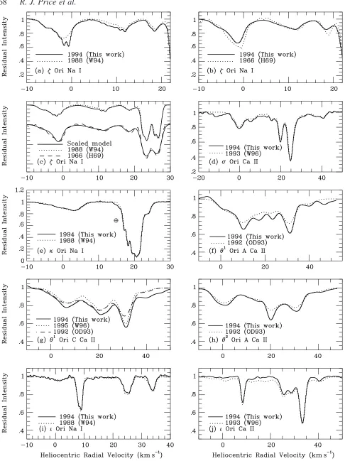
Figure 2.Comparison of our UHRF spectra with those presented in previous studies. Where spectra have been overplotted, a commoneffectiveresolving power has been used, equal to that of the lowest-resolution spectrum (detailed in Section 4). Part (c) shows a version of our NaImodel forzOri in which the column densities of components 2e† and 6† have been scaled to achieve optimum agreement with the data of H69 and W94. Residual telluric contamination is indicated by the%symbol.
and the late 1980s, followed by a factor of 1:7^0:4 increase by
1994.
Temporal variations over such a small time period imply that the absorption occurs in a spatially small parcel of gas (at least in the transverse direction). Jenkins & Peimbert (1997) and Jenkins et al.
(2000) have suggested that molecular hydrogen observed towardsz
Ori at a velocity corresponding to that of component 2e† may be produced in the compressed region behind a bow shock present in this direction (discussed further in Section 7.3).
Although the presence of a shock may account for the observed temporal variability, a small tangential displacement of the cloud,
or the line of sight, as a result of the proper motion ofzOri, causing
a shift in the line of sight probed, provides an equally likely
explanation (as invoked fordOri in Paper I). In the case ofzOri
(which has a proper motion of 4.73 mas yr21; ESA 1997), the
increase in column density of component 2e† between approxi-mately 1988 and 1994 highlights the presence of structure in the
ISM down to scales of<7 au. Indeed, Lauroesch, Meyer & Blades
(2000) have also observed temporal variability in NaItowards HD
32039/40 over scales of <15–21 au (inferred from the proper
motion of the system). However, the analysis of Lauroesch et al. (2000) assumes the cloud to be stationary. By assuming a plausible
upper limit of 50 km s21for the tangential velocity of our cloud,
the linear distance traced across the cloud may be as high as
<70 au, highlighting the importance of possible cloud motion.
The narrow linewidths of these temporally variable components seem typical of small-scale structure observed elsewhere (Papers I and II and references therein).
4.3 sOrionis
A comparison of CaIIK observations towards s Ori (shown in
Fig. 2d) appears to reveal the appearance of an absorption
component, in our 1994 spectrum, at a velocity of210.85 km s21.
An examination of the original 1993 spectrum published by W96 illustrates the presence of a very weak feature at this velocity, indicating that absorption was present, but unmodelled by W96. The differences in the absorption models therefore do not represent true variability in the absorption-line profiles.
4.4 kOrionis
Exceptional agreement is seen between the NaIobservations ofk
Ori (shown in Fig. 2e) presented by W94 and this study, apart from the presence of a weak additional component in our spectrum at a
velocity of114.95 km s21. However, the18 to116 km s21range
in this spectrum does suffer from some telluric absorption. This component is most probably not variable but instead the result of some residual contamination.
4.5 u1
Orionis A and C andu2
Orionis A
Less agreement is seen between the different CaIIspectra ofu1Ori
A and C andu2
Ori A (Figs 2f – h). Comparison of the available spectra for these stars shows the overall forms of the absorption profiles to agree reasonably well, while the cores of the absorption lines are consistently deeper in the UHRF spectra, despite convolution with an appropriate Gaussian profile. This is echoed by equivalent-width measurements, which show the strength of
absorption present towards both u1 Ori A and C to be slightly
larger in the UHRF data as compared with OD93. The total CaIIK
equivalent widths reported by OD93 for u1 Ori A and C are
105:5^2 and 101^2 mA respectively, compared to 119 :2^1:9
and 120:7^1:2 mA found here. Hobbs (1978b) found the
equivalent width of CaIIK absorption towards u1 Ori C to be
120^5 mA, in good agreement with our results, while W96 quote
94:4^0:7 mA and highlight the disagreement in equivalent-width
measurements for this star. While this effect may be the result of inaccurate zero- and/or continuum-level determinations in our own
or previous studies, the saturated NaID1 absorption present in
UHRF spectra oflandf1Ori (discussed in Section 2) suggests
the uncertainty in the zero level of the UHRF data to be small. We do note the lack of a well-determined red-wing continuum in the
CaIIspectra ofu1Ori A and C andu2Ori A, which does lead to
the possibility of errors in the continuum normalization; however,
this should, if anything, act toreduceboth the measured equivalent
widths and the absorption core depths.
The NaID2spectrum ofu1Ori C published by Hobbs (1978b),
and used by OD93 in their analysis of M42, contains an absorption
feature at a velocity of 137.7 km s21. This component is
associated with CaIIabsorption seen by OD93 at139.5 km s21.
However, this NaID2 feature is in proximity to a telluric line
(Hobbs 1978a) and is likely to be the result of telluric
contamination. Furthermore, the very weak NaID2 components
observed towards u1Ori C and u2 Ori A at<216 km s21 by
Hobbs (1978b), and unexplained by OD93, are not observed here.
The originalu1Ori C andu2Ori A NaID2spectra highlight the
presence of possible telluric absorption at this velocity (also identified in the telluric template presented by Hobbs 1978a), which we confirm as having a telluric origin, using separate
[image:16.594.53.283.54.183.2]atmospheric templates of the NaID2region obtained by us.
[image:16.594.85.248.313.403.2]Figure 2–continued
Table 4. Signal-to-noise ratios achieved for observations of CHl4300 and CH1l4232, along with 2supper limits to the equivalent widths (Wl)
and column densities (N), assuming representative
bvalues of 1.7 and 2.4 km s21for the CH and CH1
lines respectively (based on previous UHRF observations; e.g. Crawford 1995).
Star Molecule S/N Wl logN
(mA˚ ) (cm22)
u1Ori C CH 52 #0.6 #11.8
u1Ori C CH1 41 #0.9 #12.0
u2Ori A CH 62 #0.5 #11.8 u2Ori A CH1 41 #0.9 #12.0
lOri CH1 65 #0.6 #11.8
f1Ori CH1 37 #1.0 #12.0
Since much of the absorption present towards these three stars is considered to arise in clouds located in proximity to M42 (see Section 7.1.3), a certain amount of temporal variability might be expected from such an energetic environment. However, attributing the observed differences in the line profiles to intrinsic variability in the absorption is difficult because of a lack of previous very high-resolution data. We conclude that there is no secure evidence as yet for significant variability in these sightlines.
4.6 iOrionis
Although W94 identify several additional weak components in
their NaIspectrum ofiOri, excellent agreement is still seen with
our observations (see Fig. 2i). With regards to the CaII region,
however, additional weak components identified by W96 do
produce a noticeable difference (see Fig. 2j); however, we feel that these differences are unlikely to be the result of temporal variability and are easily attributable to differences in continuum normalization.
4.7 bOrionis
Although a comparison of our CaIIspectrum with that presented
by Marschall & Hobbs (1972) can be made in order to search for temporal variability (Fig. 2k), the intrinsically weak nature of these lines, and the presence of a strong stellar line, both create problems with this procedure. The strength of the absorption present around
0 km s21appears similar in both studies, but that near19 km s21
(our cloud 7a) appears somewhat weaker in the Marschall & Hobbs data, indicating possible temporal variability in this component. As discussed in Section 7.4, variability, coupled with ongoing mass loss, suggests a circumstellar origin. Further absorption, below a
velocity of 210 km s21, is also thought to arise within the
circumstellar environment of b Ori (Section 7.4), but an
insufficient blueward range in the Marschall & Hobbs (1972) spectrum does not permit a comparison for these components.
5 C L O U D K I N E T I C T E M P E R AT U R E S A N D T U R B U L E N T V E L O C I T I E S
Interstellar line broadening is dominantly the result of two effects, namely Doppler broadening due to (a) the kinetic temperature of
the absorbers,Tk, and (b) the line-of-sight rms turbulent velocity
within the cloud,vt. If the velocity spectrum of the turbulence is
Gaussian, then the bvalue resulting from these two broadening
mechanisms is described by
b¼
ffiffiffiffiffiffiffiffiffiffiffiffiffiffiffiffiffiffiffiffiffiffiffi
2kTk
m 12v
2 t
r
; ð1Þ
where the observed line FWHM¼1:665b, k is Boltzmann’s
constant andmis the mass of the relevant atom/ion (see Cowie &
Songaila 1986). Thus by observing two species that are considered to exist co-spatially, and which have an adequate mass differential, e.g. Na and K, it becomes possible to solve equation (1)
simultaneously for bothTkandvt(see Dunkin & Crawford 1999).
Where the best-fitting b values of corresponding NaI and KI
components provide a solution to equation (1), ‘exact solutions’ are
said to be obtained (see columns 7–10 of Table 5). Furthermore, 1s
error limits quoted in Table 3 have also been adopted for eachb
value, providing a range of allowed solutions to equation (1) (see
columns 11–14 of Table 5). Since these calculations depend Table
5. V alues of kin etic temper ature ( Tk ), turb ulen t v eloci ty ( vt ), three-di mensio nal turb ulent v elocity ð ; ffiffiffi 3 p vt Þ an d iso thermal sound speed ( Cs ; relating to atomi c H with 10 per cent He by number) for clouds simultan eously observ ed in two co-e xtensi v e species. Co lumns 1, 2 and 3 sho w the sig htline studied and its tota l co lumn densiti es of H I an d H2 .Column 4 display s the spec ies used in the analy sis, while co lumns 5 and 6 display the componen t number and the heliocent ric rad ial v eloci ty (taken from the Na I counter part, as listed in T able 3). Co lumns 7–10 display ex act solutions , wher e av ail able, while column s 11–14 dis play all v alues all o w ed within the 1 s error limits quoted in T able 3. In the cas es where no solutions within the 1 s error bounds are av ailable, 2 s error limits are in v oked an d the results are discussed in the te xt. Star log [ N ]tot Method Cloud v( Tk vt ffiffiffi 3 p vt Cs D Tk D vt D ffiffiffi 3 p vt D Cs [H] [H 2 ] (km s 2 1 ) (K) (k m s 2 1 ) (km s 2 1 ) (km s 2 1 ) (K) (k m s 2 1 ) (km s 2 1 ) (km s 2 1 ) 1 2 3 4 5 6 7 8 9 1 0 1 1 1 21 31 4 e Ori 20.45 16.5 7 Na I /Ca II 2 2.90 86 0.17 0.30 0.75 22 – 148 0.11 – 0.22 0.18 – 0.39 0.38 – 0.98 Na I /K I 5 10.94 355 0.26 0.46 1.52 0 – 584 0.00 – 0.43 0.00 – 0.75 0.00 – 1.96 Na I /K I 11 24.77 77 0.37 0.65 0.71 0 – 404 0.18 – 0.42 0.32 – 0.73 0.00 – 1.63 z Ori 20.41 15.7 3 Na I /K I 2e† 2 1.07 – – – – 0 – 293 0.00 – 0.33 0.00 – 0.56 0.00 – 1.38 Na I /K I 8a 22.97 – – – – – – – – Na I /K I 8b 23.19 – – – – – – – – Na I /K I 11a 26.20 – – – – 0 – 101 0.00 – 0.19 0.00 – 0.33 0.00 – 0.81 Na I /K I 11b 26.41 – – – – 508 – 841 0.00 – 0.30 0.00 – 0.52 1.82 – 2.35 k Ori 20.52 15.6 8 Na I /K I 6 17.76 – – – – – – – – Na I /K I 7 18.86 – – – – 0 – 280 0.00 – 0.32 0.00 – 0.55 0.00 – 1.35 Na I /K I 8 20.25 356 0.34 0.59 1.53 0 – 757 0.00 – 0.52 0.00 – 0.91 0.00 – 2.23 Na I /K I 9 21.05 – – – – 0 – 244 0.00 – 0.30 0.00 – 0.51 0.00 – 1.26
critically on the component structures obtained from our models, this type of analysis is best suited to isolated velocity components, where confusion with nearby blended absorption is at a minimum.
Furthermore, for the intrinsically weak KIline to be detectable, the
NaID1line must be strong, but not saturated. In order for these
results to be meaningful, the intrinsic widths of the lines must be determined, something best suited to very high-resolution, high signal-to-noise ratio data.
The derived value ofTkcan subsequently be used to determine
the isothermal sound speed,Cs, in a cloud, using the relation
Cs¼
ffiffiffiffiffiffiffiffi
kTk
m s
; ð2Þ
wheremis the mean mass per particle, here assumed to be 1.27mH,
i.e. an atomic H gas containing 10 per cent He by number (e.g. Spitzer 1978). Positive detections of molecular hydrogen have
been made towardse,zandkOri at velocities corresponding to
each KI component (see fig. 3 of Jenkins et al. 2000; fig. 7 of
Jenkins & Peimbert 1997; and table 1 of Spitzer & Morton 1976). The presence of molecular hydrogen in these clouds will of course increase the mean mass per particle, therefore reducing the prevailing isothermal sound speed; however, the column densities of molecular hydrogen are seen to be small with respect to those of
hydrogen (total HIand H2column densities are shown in Table 5,
taken from Savage et al. 1977). In reality H2 is likely to be
preferentially found in the same (colder/denser) regions where the
NaI and KI absorption is thought to arise, but the fraction of
hydrogen in the molecular form is still expected to be small. Even if 50 per cent of the H atoms in these regions were to be in the
molecular form,mwill be 1.65mH, only resulting in an<14 per
cent decrease inCs.
Observations of both NaI and KI have been made for the
sightlines towards b, e, z and k Orionis, which we discuss
below.
5.1 bOrionis
Absorption from KIhas not been positively identified towardsb
Ori. This is consistent with the relatively weak strength of NaI
towards this star. Although our sample of NaI, KIpairs is far too
small for a meaningful statistical analysis, a comparison of Na0and
K0column densities shows a typical ratio Na0/K0<60, leading to
an expected K0column density towardsbOri of only logN<9:00
from the strongest NaI component, which is below our detection
threshold.
5.2 eOrionis
Observations of KItowardseOri reveal the presence of two main
components. The higher-velocity component exhibits slight asymmetry, although it can be accurately modelled with a single absorbing cloud. Exact solutions are achievable for both clouds and
show bothvtand
ffiffiffi
3
p
vtto be subsonic. Only in the extreme case
where the majority of H is present in the molecular form does the
sound speed of e Ori’s 124.77 km s21 component permit
supersonic, three-dimensional turbulent motions. Over the full
1s error range, supersonic turbulence is only permitted whenTk
resides near its lower limit.
A very narrow NaI absorption component with one of the
clearest examples of HFS is present at a velocity of
12:90^0:01 km s21. Although too weak to be accurately
modelled, a possible signature of KI absorption is present at a
similar velocity ð<12:7 km s21Þ, with an equivalent width of
#0.5 mA˚ . Furthermore, a comparison of the NaIand CaIIspectra
of e Ori illustrates a narrow CaII absorption component at a
velocity of12:88^0:01 km s21. This system is a clear example of
both NaI and CaII absorption from a cool cloud occurring at
(within the errors) the same velocity. By assuming the case of
purely thermalðvt¼0Þor purely turbulentðTk¼0Þbroadening, it
is possible to place strict upper limits on both the Tk and vt
prevailing in the regions where the NaI and CaII absorption is
occurring, without having to assume that the species are co-spatial.
In the case of Na0,Tk#169 K andvt#0:25 km s21, while for
Ca1,Tk#231 K andvt#0:22 km s21.
It is generally observed that line broadening in CaII is greater
than that seen in NaI(interpreted to be due to Ca1preferentially
occupying the warmer outer regions of a cloud; e.g. Barlow et al.
1995). However, in this case it is NaI that is seen to exhibit the
largest broadening. The fact that the lighter Na atom is subjected to greater broadening may signify that the species exist co-spatially. This being the case, it is possible to solve equation (1) in the same
way as has been done for NaIand KI(see first entry of Table 5).
Both the line-of-sight and three-dimensional turbulent velocities are well below the corresponding sound speeds for either a purely atomic or a purely molecular gas, indicating the turbulence to be subsonic in all cases. We find that three-dimensional supersonic
turbulent motions are only permitted in an atomic gas whenTkisat
its lower limit. It is interesting to note that, while this cloud is cold,
it has a Na0/Ca1
ratio of 1.78, illustrating that not all the Ca has been depleted. Since Ca is rapidly depleted on to grain surfaces (Barlow et al. 1995), the recent removal of Ca atoms from grains would be implied, consistent with Na and Ca being co-extensive.
5.3 zOrionis
Between velocities of120 and130 km s21, the IS NaIspectrum
of z Ori is dominated by two features. Modelling of these two
features requires five components for a satisfactory fit.
Examin-ation of this star’s KIIS spectrum echoes the presence of the two
major NaI features, but further investigation reveals the
components to be asymmetric, such that four of the five NaI
components have corresponding KI components. The highly
blended nature of this region leads, in general, to larger errors for
the weak KI components. An additional weak KI component is
also present at 21.31 km s21, corresponding to the temporally
variable NaIcomponent at21.07 km s21(see Section 4.2).
None of the velocity components permit exact solutions forTk
and vt, while clouds 8(a) and 8(b) do not allow any physical
solutions within their respective 1serror ranges. In this case, 2s
error ranges can be applied, resulting in an allowed range forTk
and vtfor both clouds. Within the 2serror range of cloud 8(a),
Tk,92 K while 0:18,vt,0:25. In the case of cloud 8(b),Tk,
1023 K andvt,0:61. In the case of cloud 11(b), the line-of-sight
and three-dimensional turbulence is subsonic, even in a molecular gas. For the remaining clouds, supersonic turbulence is only
allowed whenTkis near its lower limit.
5.4 kOrionis
Observations of KI towards k Ori reveal the presence of two
absorption features, near 118 and 120 km s21. Although both
regions can be accurately fitted with a single component, the
120 km s21feature coincides with three strong NaI components
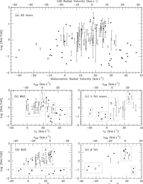
Figure 3.Na0to Ca+column density ratios plotted as a function of radial velocity (upward- and downward-pointing triangles represent lower and upper limits, respectively). Part (a) shows all clouds identified towards the Orion stars, and parts (b) – (e) display clouds identified in selected sightlines, and illustrate the broad groupings discussed in Section 6. The groupings are complete in the most part; however, there are a small number of instances where it has not been possible to include points in their correct group.
and so has been modelled with three corresponding KI components.
Only cloud 8 permits exact solutions forTkandvt, while cloud 6
has no physical solutions within its 1serror range. If 2serrors are
applied to cloud 6, we findTk,332 K andvt,0:32. Supersonic
turbulence is again only permitted whenTkis near its lower limit.
A comparison ofvtand ffiffiffi3
p
vtwithCsfrom the available exact
solutions to equation (1) (Table 5, columns 7–10Þdemonstrates the
turbulent motions to be subsonic in all cases. If a molecular gas is
assumed, only e Ori’s cloud 11 permits supersonic
three-dimensional turbulent motions, if 50 per cent or more of the H
nuclei are in the form of H2.
Similarly, where exact solutions are not available, a comparison of the range of turbulent velocities and sound speeds permitted
within the adoptedbvalue error ranges (shown in Table 5, columns
11–14Þindicates that the turbulent motions are generally subsonic,
unlessTk is near its lower limit. However, this is subject to a
selection effect. In the two extreme cases where eitherTkorvtis
zero, we find that the allowedbvalues of the two observed species
range from being equal to differing by a factor equal to the square root of their mass ratio, respectively. Outside this range, no physical solutions are permitted. Since the errors associated with
thebvalues of KIare in general much larger than those of their
NaIcounterparts (weaker components, lower S/N), solutions forTk
andvtare available for eachbvalue allowed within the 1serror
range of several NaIcomponents [clouds 2e† and 11a towardsz
Ori and clouds 7, 8 (although an exact solution is available for this
cloud) and 9 towards k Ori]. This illustrates that the line
broadening in both species should be determined to a level of
accuracy such that solutions forTkandvtare not obtainable over
the entire range of permittedbvalues of either of the species. If this
is not achieved, the range of permitted values ofTkandvtis not
restricted any further than that which may be obtained from the observation of a single species.
Where solutions forTk and vtare available for each bvalue
within the NaI error range, 95 and 92 per cent of these possible
solutions describe subsonic turbulence in purely atomic and purely molecular gas, respectively. When considering the perhaps more
realistic case of three-dimensional turbulence ð; ffiffiffi3
p
vtÞ, these
values fall to 87 and 79 per cent, again for a purely atomic and a purely molecular gas, respectively. This illustrates that, in these cases, the range of permitted values will inherently show
turbulence to remain subsonic unlessTkresides near its lower limit.
6 N A0/ C A1A B U N D A N C E R AT I O S
It has long been recognized that interstellar absorption components
display a very wide range of Na0/Ca1
ratios. This is primarily due to variations in the gas-phase abundance of Ca, governed by a balance between preferential Ca adsorption on to grain surfaces in quiescent dense environments, and removal from grain surfaces by shocks and sputtering in energetic environments (e.g. Jura 1976; Barlow & Silk 1977; Barlow 1978; Phillips, Pettini & Gondhalekar
1984). Although interpretation is complicated by the fact that Ca1
and Na0 do not necessarily dominate in the same regions of an
interstellar cloud (e.g. Barlow et al. 1995), in those cases where an
origin in the same cloud can plausibly be assumed, the Na0/Ca1
ratio can yield information on the prevailing physical conditions (Crawford 1992).
Na0/Ca1 ratios have been calculated for each of the clouds
identified in these data (column 5, Table 3). Where a single NaI
component corresponds well to a single CaII component, a
Na0/Ca1ratio is derived for the cloud. Where one or more NaI
components correspond to one or more CaIIcomponents, a mean
Na0/Ca1ratio is given for the system as a whole. Error limits on
the ratio are found by calculating the range of Na0/Ca1 ratios
allowed within the error bounds of the Na0 and Ca1 column
densities. In the situation where a NaIor CaIIcomponent has no
corresponding CaIIor NaIcomponent, lower and upper limits to
the Na0/Ca1 ratio are given by calculating upper limits to
associated absorption that may be present but undetected.
Following Welsh et al. (1990) the 2supper limit to the equivalent
width,Wl, of an undetected line is found assuming
Wl&
2Dl ffiffiffiffiffiffiffiffiffiffiNcont
p
S=N ; ð3Þ
whereDlis the width of one data pixel in A˚ ,Ncontis the assumed
width, in the continuum, of the undetected absorption line in pixels, and S/N is the continuum signal-to-noise ratio of the observation.
Here, the FWHM of a CaII line has been taken to be 1.3 times
larger than that of a corresponding NaI line (found through the
comparison of all CaII, NaIpairs in Table 3) and the linewidth in
the continuum is taken to be 2.5 times larger than the FWHM. The column density of the line is then found assuming
N&1:131020Wl
fl2; ð4Þ
wherefis the oscillator strength of the transition (see Table 2) and
Wland l are both given in A˚ (Cowie & Songaila 1986). If an
‘undetected’ line is present in a blended region, the upper limit
derived forNmay be slightly underestimated.
Fig. 3(a) displays all calculated Na0/Ca1ratios as a function of
radial velocity (taken as a mean of the constituent components). Figs 3(b) – (e) show similar individual plots for the M42 region, the
lOri association, the Belt stars andbOri, respectively. Velocities
with respect to the local standard of rest (LSR) and the Sun are marked at the top and bottom of each figure, respectively.
When considering Fig. 3(a) in terms of LSR radial velocities, a
clear illustration of the fall-off of the Na0/Ca1ratio with absolute
radial velocity can be seen (Routly & Spitzer 1952). However, while Routly & Spitzer (1952) surmised that clouds with small
Na0/Ca1 ratios are preferentially found at larger absolute
velocities, further investigation of Fig. 3(a) shows such clouds to be distributed throughout the velocity range. The situation is
therefore more likely to be that clouds with small Na0/Ca1ratios
possess a larger distribution of velocities. Furthermore, additional
clouds characterized by low Na0/Ca1
ratios are likely to be present at low absolute velocities but simply masked by the much stronger absorption from the colder/denser clouds that generally occupy these velocities. A similar effect was noted by Crawford, Barlow & Blades (1989) in their study of the ISM towards the Sco OB1 association.
Anticipating the discussion in the next section, many of the points in Figs 3(b) – (e) have been collected together into broad groups of clouds possessing similar characteristics. These groups are labelled with letters, representing: A) cold diffuse/molecular
clouds B) warm intercloud gas C) possible mass-loss material D)l
Ori shell material E) M42 neutral lid F) M42 foreground clouds G)
HIIregion(s) foreground to M42.
An inspection of the average radial velocities of cold
diffuse/partially molecular clouds with larger Na0/Ca1 ratios
(group A) highlights a small systematic change in radial velocity.
In the south,k Ori exhibits its strongest NaI absorption around