A Class of Iterative Methods for Solving Nonlinear Equations with Optimal Fourth order Convergence

A Class of Iterative Methods for Solving Nonlinear

Equations with Optimal Fourth-order Convergence

J. P. Jaiswal

Department of Mathematics, Maulana Azad National Institute of Technology, Bhopal, M.P., 462051, India

∗_{Corresponding Author: [email protected]}

Copyright c⃝2014 Horizon Research Publishing All rights reserved.

Abstract

In this paper we construct a new third-order iterative method for solving nonlinear equations for simple roots by using inverse function theorem. After that a class of optimal fourth-order methods by using one function and two first derivative evaluations per full cycle is given which is obtained by improving the existing third-order method with help of weight function. Some physical examples are given to illustrate the efficiency and performance of our methods.

Keywords

Newton Method, Order of Convergence, Optimal Order, Inverse Function, Weight Function

Mathematics Subject Classification (2000).

41A25, 65D99

1

Introduction

Nonlinear equations plays an important role in science and engineering. Finding an analytic solution is not always possible. Therefore, numerical methods are used in such situations. The classical Newton’s method is the best known iterative method for solving nonlinear equations. To improve the local order of convergence and efficiency index, many modified third-order methods have been presented in literature. For detail we refer [[16], [9], [1], [15], [5]] and references therein.

Recently Ardelean [3] establishedBisectrix Newton’s Method (BN), which is given by xn+1=xn−

(f′(xn) +f′(yn))f(xn)

f′(xn)f′(yn) +

√

(1 +f′(xn)2)(1 +f′(yn)2)−1

, n≥0, (1.1)

whereyn=xn− f(xn)

f′(xn). The method is third-order convergent for simple roots and its efficiency index is3

1/3_{= 1.4422.}

Weerakoon et al. [16] used Newton’s theorem

f(x) =f(xn) +

∫ x

xn

f′(t)dt (1.2)

and approximated the integral by trapezoidal rule, i.e.

∫ x

xn

f′(t)dt=(x−xn) 2 [f

′_(x

n) +f′(x)], (1.3)

obtained the following variant of the Newton method xn+1=xn−

2f(xn)

f′(xn) +f′(yn)

, (1.4)

whereyn = xn − _ff′((xxnn)). It is shown that this is third-order. Many authors used this idea to approximate the integral

∫x xnf

′_{(t)dtby different rule. For more detail, one can see [ [12], [13], [14], [8], [9], [15], [5] ] and the references there in.} If we approximated the integral in(1.2)by

∫ x

xn

f′(t)dt= (x−xn)

[

f′(xn)f′(x) +

√

(1 +f′(xn)2)(1 +f′(x)2)−1

(f′(xn) +f′(x))

]

we get the same formula(1.1).

Next Homeier [9] used Newton’s theorem(1.2)for the inverse functionx=f−1_{(y) =g(y)instead ofy=f(x), that is}

g(y) = g(yn) +

∫ y

yn

g′(s)ds. (1.6)

Then the method(1.4)takes the form

xn+1=xn−

f(xn)

2

[

1

f′(xn)

+ 1

f′(yn)

]

, (1.7)

whereyn =xn−_ff′((xxnn)). This method is again third-order.

Here we state following definitions:

Definition 1.1. Let f(x) be a real function with a simple rootαand letxn be a sequence of real numbers that converge

towardsα. The order of convergence m is given by

lim

n→∞

xn+1−α

(xn−α)m

=ζ̸= 0, (1.8)

whereζis the asymptotic error constant andm∈R+_.

Definition 1.2. Letβbe the number of function evaluations of the new method. The efficiency of the new method is measured

by the concept of efficiency index [17, 11] and defined as

µ1/β, (1.9)

whereµis the order of the method.

Kung and Traub [10] presented a hypothesis on the optimality of roots by giving2n−1as the optimal order. This means that the Newton iteration by two evaluations per iterations is optimal with 1.414 as the efficiency index. By taking into account the optimality concept many authors have tried to build iterative methods of optimal higher order of convergence.

This paper is organized as follows: in section 2, we describe the new third-order iterative method by using the concept of inverse function theorem. In the next section we optimize the method of Chun et. al [4] with help of weight function. Finally in the last section we give some physical example and our new methods are compared in the performance with some well known methods.

2

Development of the method and convergence analysis

In this section we use the concept of inverse function to derive variants of Bisectrix Newton’s Method. In the formula

(1.1), functiony =f(x)has been used. Here we use inverse functionx=f−1(y) =g(y)instead ofy =f(x). Then we have

g(y) = g(yn) +

∫ y

yn

g′(s)ds

= g(yn) + (y−yn)

[

g′(yn)g′(y) +

√

(1 +g′(yn)2)(1 +g′(y)2)−1

(g′(yn) +g′(y))

]

,

(2.1) whereyn =f(xn). Now using the fact thatg′(y) = (f−1)

′

(y) = [f′(x)]−1_{and thaty=f(x) = 0, we obtain the following}

method:

xn+1=xn−f(xn)

[

1 +√(1 +f′(xn)2)(1 +f′(yn)2)−f′(xn)f′(yn)

f′(xn) +f′(yn)

]

. (2.2)

where

yn =xn−

f(xn)

f′(xn)

. (2.3)

Now we prove that order of convergence of this method is also three.

Theorem 2.1. Let the function f have sufficient number of continuous derivatives in a neighborhood ofαwhich is a simple

Proof. Leten=xn−αbe the error in thenthiterate andch= f(h)_(α)

h! ,h= 1,2,3.... We provide the Taylor series expansion

of each term involved in(2.2). By Taylor expansion around the simple root in thenth_{iteration, we have}

f(xn) =f′(α)[en+c2e2n+c3e3n+c4e4n+c

5 5e

5

n+c6e6n+O(e

7

n)] (2.4)

and, we have

f′(xn) =f′(α)[1 + 2c2en+ 3c3e2n+ 4c4e3n+ 5c

5 5e

4

n+ 6c6e5n+O(e

6

n)]. (2.5)

Further more it can be easily find f(xn

f′(xn)

=en−c2e2n+ (2c

2

2−2c3)e3n+...+O(e

6

n). (2.6)

By considering this relation, we obtain

yn=α+c2en2 + 2(c3−c22)e 3

n+...+O(e

6

n). (2.7)

At this time, we should expandf′(yn)around the root by taking into consideration(2.7). Accordingly, we have

f′(yn) =f′(α)[1 + 2c22e 2

n+ (4c2c3−4c32)e 3

n+...+O(e

6

n)]. (2.8)

By consider the above mentioned relations(2.4),(2.5)and(2.8)in the equation(2.2), we can find

en+1= (

c2₂

1 +f′(α)2 +

c3

2

)

e3_n+O(e4_n). (2.9)

This confirms the result.

3

Optimal fourth-order iterative method

By using circle of curvature concept Chun et. al. [4] constructed a third-order iterative methods defined by

yn = xn−

f(xn)

f′(xn)

,

xn+1 = xn−

1 2

[

3−f

′_(yn) f′(xn)

]

f(xn)

f′(xn)

. (3.1)

The order of this method three is with three (one derivative and two function) evaluations per full iteration. Clearly its efficiency index(31/3≈1.4422)is not high (optimal=(41/3≈1.5844). We now make use of weight function approach to build our optimal class based on(3.1)by a simple change in its first step. Thus we consider

yn = xn−a

f(xn)

f′(xn)

,

xn+1 = xn−

1 2

[

3−f

′_(y

n)

f′(xn)

]

f(xn)

f′(xn)×

G(t). (3.2)

whereG(t)is a real-valued weight function witht= f′(yn)

f′(xn) andais a real constant. The weight function should be chosen

such that order of convergence arrives at optimal level four without using more function evaluations. The following theorem indicates under what conditions on the weight functions and constantain(3.2), the order of convergence will arrive at the optimal level four:

Theorem 3.1. Let the function f have sufficient number of continuous derivatives in a neighborhood ofαwhich is a simple

root of f, then the method(3.2)has fourth-order convergence, whena = 2/3 and the weight functionG(t)satisfies the following conditions

G(1) = 1, G′(1) = −1 4 , G

′′

(1) = 2,G(3)(1)≤+∞, (3.3)

and the error equation is given by(3.8).

Proof. Using(2.4)and(2.5)anda= 2/3in the first step of(3.2), we have

yn=α+

en

3 + 2c2e2n

3 +

4(c3−c22)e3n

3 +...+O(e

6

Now we should expandf′(yn)around the root by taking into consideration(3.4).Thus, we have

f′(yn) =f′(α)

[

1 + 2c2en 3 +

(4c2

2+c3)e2n

3 +...+O(e

6

n)

]

. (3.5)

Furthermore, we have

f′(yn)

f′(xn)

= 1−2c2 3 en+

(

4c2₂−8c3

3

)

e2_n+...+O(e6_n). (3.6)

By virtue of(3.6)and(3.3), we attain

1 2

[

3−f

′_(y

n)

f′(xn)

]

f(xn)

f′(xn)

×G(t)

=en+

[

c2c3−

c4

9 +− 1

81{309 + 32H

(3)_(1)}c3 2 ]

e4_n+O(e5_n). (3.7)

Finally using(3.7)in(3.2), we can have the following general equation, which reveals the fourth-order convergence en+1=xn+1−α

=xn−

1 2

[

3− f

′_(y

n)

f′(xn)

]

f(xn)

f′(xn)

×G(t)−α

=

[

−c2c3+

c4

9 + 1

81{309 + 32G

(3)_(1)}c3 2 ]

e4_n+O(e5_n). (3.8)

This proves the theorem.

It is obvious that our novel class of iterations requires three evaluations per iteration, i.e. two first derivative and one function evaluations. Thus our new methods are optimal. Now by choosing appropriate weight functions as presented in

(3.2), we can give number of optimal two-step iterative methods. Here we are giving one of them as follows:

yn = xn−

2 3

f(xn)

f′(xn)

,

xn+1 = xn−

1 2

[

3−f

′_(yn) f′(xn)

] [

9 4−

9 4

f′(yn)

f′(xn)

+

(

f′(yn)

f′(xn)

)2]

f(xn)

f′(xn)

. (3.9)

where its error equation is

en+1= [

−c2c3+

c4 9 + 309 81 c 3 2 ]

e4_n+O(e5_n). (3.10)

4

Examples

In this section we give some physical examples and compare our methods with other some well known methods. Here all the computations have been done by using Mathematica8. We consider the number of decimal places as follows:200digits floating point(SetAccuracy= 200)with SetAccuracy command. The test of examples from(4.1)to(4.3)are listed in the Table1to3respectively. We compare the performance of our third-order method (M1)(2.2)and fouth-order (M2)(3.10)

method with Newton method (NM), Weerakkon method (WKM)(1.4), Hommeier method (HMM)(1.7), Bisectrix Newton method (BNM)(1.1), Chun method (CHM)(3.1), method(6)(KHM) of [18] and method(17)(SNM) of [7] respectively.

Example 4.1[2] Consider Plank’s radiation law

ϕ(λ) = 8πchλ

−5

ech/λkT −₁,

whereλis the wavelength of the radiation,tis the absolute temperature of the blackbody,kis Boltzmann’s constant,his the Planck’s constant andcis the speed of light. This formula calculate the energy density within an isothermal blackbody. Now we want to find wavelengthλwhich maximize energy densityϕ(λ). For maximum ofϕ(λ), it can easily seen that

(ch/λkT)ech/λkT ech/λkT −₁ = 5.

Letx=ch/λkT, then it becomes

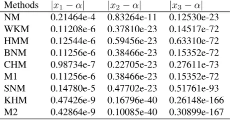
Table 1.Errors Occurring in the estimates of the root of functionf1by the methods described below with initial guessx0= 5.

Methods |x1−α| |x2−α| |x3−α|

NM 0.21464e-4 0.83264e-11 0.12530e-23 WKM 0.11208e-6 0.37810e-23 0.14517e-72 HMM 0.12544e-6 0.59456e-23 0.63310e-72 BNM 0.11256e-6 0.38466e-23 0.15352e-72 CHM 0.98734e-7 0.22705e-23 0.27611e-73 M1 0.11256e-6 0.38466e-23 0.15352e-72 SNM 0.14780e-5 0.47702e-23 0.51761e-93 KHM 0.47426e-9 0.16796e-40 0.26148e-166 M2 0.42864e-9 0.10085e-40 0.30899e-167

Now the above equation can be rewritten as

f1(x) =e−x−1 +x/5. (4.2)

Our aim to find the root of the equationf1(x) = 0. Clearly zero is its one root, which is not of our interest. If we takex= 5,

then R.H.S. of(4.2)becomes zero and L.H.S. ise−5≈6.74×10−3. This implies one root of the equationf1(x) = 0is near

to 5. So that here we compare some well known methods to our methods with initial guess 5, which are given in table 1.

Example 4.2[6] The depth of embedmentxof a sheet-pile wall is governed by the equation:

x=x

3_{+ 2.87x}2_−10.28

4.62 .

It can be rewritten as

f2(x) =

x3_{+ 2.87x}2_−10.28

4.62 −x.

An engineer has estimated the depth to bex= 2.5. Here we find the root of the equationf2(x) = 0with initial guess 2.5 and

[image:5.595.189.421.73.194.2]

compare some well known methods to our methods, which are given in table 2.

Table 2.Errors Occurring in the estimates of the root of functionf2by the methods described below with initial guessx0= 2.5.

Methods |x1−α| |x2−α| |x3−α|

NM 0.85925e-1 0.32675e-2 0.50032e-5 WKM 0.18271e-1 0.14770e-5 0.79610e-18 HMM 0.49772e-2 0.33027e-8 0.95318e-27 BNM 0.54594e-2 0.63617e-8 0.10016e-25 CHM 0.27815e-1 0.95903e-5 0.41254e-15 M1 0.54594e-2 0.63617e-8 0.10016e-25 SNM 0.26594e-1 0.32982e-6 0.76311e-26 KHM 0.14965e-1 0.45484e-7 0.40826e-29 M2 0.80338e-2 0.15138e-8 0.19455e-35

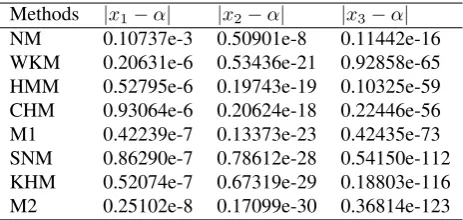
Example 4.3[6] The vertical stressσz generated at point in an elastic continuum under the edge of a strip footing

sup-porting a uniform pressureqis given by Boussinesq’s formula to be: σz=

q

π{x+Cosx Sinx}

A scientist is interested to estimate the value ofxat which the vertical stressσzwill be 25 percent of the footing stressq.

Initially it is estimated thatx= 0.4. The above can be rewritten as forσzis equal to 25 percent of the footing stressq:

f3(x) =

x+Cosx Sinx

π −

1 4.

Now we find the root of the equationf3(x) = 0with initial guess 0.4 and compare some well known methods to our

[image:6.595.174.406.71.181.2]

Table 3.Errors Occurring in the estimates of the root of functionf3by the methods described below with initial guessx0= 0.4.

Methods |x1−α| |x2−α| |x3−α|

NM 0.10737e-3 0.50901e-8 0.11442e-16 WKM 0.20631e-6 0.53436e-21 0.92858e-65 HMM 0.52795e-6 0.19743e-19 0.10325e-59 CHM 0.93064e-6 0.20624e-18 0.22446e-56 M1 0.42239e-7 0.13373e-23 0.42435e-73 SNM 0.86290e-7 0.78612e-28 0.54150e-112 KHM 0.52074e-7 0.67319e-29 0.18803e-116 M2 0.25102e-8 0.17099e-30 0.36814e-123

5

Conclusion

In this present paper we have given a new third-order and a class of the optimal fourth-order iterative methods for simple roots for solving nonlinear equations. The third-order method is obtained by using inverse function theorem and the class op-timal fourth-order method is obtained with help of weight function using in the existing third-order method without using any function evaluations. Three physical examples are given to illustrate the superior performance of our methods by comparing them with some well existing third and fourth-order iterative methods.

REFERENCES

[1] A. Y. Ozban: Some new variants of Newton’s method, Appl. Math. Letter, 17 (2004), 677-682. [2] B. Bradie: A Friendly Introduction to Numerical Analysis, Pearson Education Inc, New Delhi, (2006).

[3] C. Ardelean: A new third-order Newton-type iterative method for solving nonlinear equations, Appl. Math. Comput. 219 (2013), 9856-9864.

[4] C. Chun and Y. I. Kim: Several new third-Order iterative methods for solving nonlinear equations, Acta Appl. Math. 109 (2010), 1053-1063.

[5] D. Jain: Families of Newton-like methods with fourth-order convergence, International Journal of Computer Mathemat-ics, 90 (5) (2013), 1072-1082.

[6] D. V. Griffithms and I. M. Smith: Numerical methods for engineers, Second Edition, Chapman and Hall/CRC (Taylor and Francis Grpup), Special Indian Edition (2011).

[7] F. Soleymani: Two new classes of optimal Jarratt-type fourth order methods, Applied Mathematics Letter, 25 (2012), 847-853.

[8] H. H. H. Homeier: A modified Newton method for root finding with cubic convergence, J. Comput. Appl. Math. 157 (2003), 227-230.

[9] H. H. H. Homeier: On Newton-type methods with cubic convergence, J. Comput. Appl. Math. 176 (2005), 425-432. [10] H. T. Kung and J. F. Traub: Optimal order of one-point and multipoint iteration, JCAM 21 (1974), 643-651 . [11] J. F. Traub: Iterative methods for solution of equations chelsea Publishing, New York, NY, USA (1997).

[12] M. Frontini: Hermite interpolation and a new iterative method for the computation of the roots of non-linear equations, Calcolo 40 (2003), 109-119.

[13] M. Frontini and E. Sormani: Modified Newton’s method with third-order convergence and multiple roots, J. Comput. Appl. Math. 156 (2003), 345-354.

[14] M. Frontini and E. Sormani: Some variant of Newton’s method with third-order convergence, Appl. Math. Comput. 140 (2003), 419-426.

[15] P. Wang: A third-order family of Newton-like iteration methods for solving nonlinear equations, J. Numer. Math. Stoch. 3 (2011), 13-19.

[16] S. Weerakoon, T. G. I. Fernando: A variant of Newton’s method with accelerated third-order convergence, Appl.Math. Lett.13 (2000) 87-93.