Stability Analysis of Higher Order Delta Sigma Modulators for Dual Sinusoidal Inputs

University of East London Institutional Repository: http://roar.uel.ac.uk

This paper is made available online in accordance with publisher policies. Please scroll down to view the document itself. Please refer to the repository record for this item and our policy information available from the repository home page for further information.

To see the final version of this paper please visit the publisher’s website. Access to the published version may require a subscription.

Author(s):

Lota, Jaswinder. Al-Janabi, Mohammed., Kale, Izzet

Article Title:

Stability Analysis of Higher-Order Delta-Sigma Modulators for Dual Sinusoidal Inputs

Year of publication:

2007

Citation:

Lota, J. Al-Janabi, M., Kale, I. (2007) ‘Stability analysis of higher-order delta-sigma modulators for sinusoidal inputs.’In: Proceedings of the IEEE

Instrumentation and Measurement Technology Conference, Warsaw, Poland, May 1-3, 2007. IEEE, Los Alamitos, USA, pp. 1-5. ISBN 1424405882

Link to published version:

http://www.ieee.org/web/publications/books/index.html

DOI:

(not stated)

Publisher statement:

Stability Analysis of Higher-Order Delta-Sigma

Modulators for Dual Sinusoidal Inputs

Jaswinder Lota*, MIEEE, Mohammed Al-Janabi*, MIEEE, Izzet Kale*+, MIEEE

*Applied DSP and VLSI Research Group, Department of Electronic Systems, University of Westminster, London, UK

+

Applied DSP and VLSI Research Centre, EasternMediterranean University, Gazimagusa, Mersin 10, Turkey [email protected], [email protected], [email protected]

Abstract- The aim of this paper is to determine the stability of higher-order ∆-Σ modulators for sinusoidal inputs. The nonlinear gains for the single bit quantizer for a dual sinusoidal input have been derived and the maximum stable input limits for a fifth-order

Chebyshev Type II based ∆-Σ modulators are

established. These results are useful for optimising the design of higher-order ∆-Σ modulators.

I. INTRODUCTION

The stable input amplitude limits for ∆-Σ modulators is complicated to predict due to the non-linearity introduced by the quantizer in the feedback loop. Various approaches have been employed to explain this nonlinear behaviour. Using quasilinear modeling, a new interpretation of the instability mechanism for ∆-Σ modulators based on the noise amplification curve is given in [1]. This is restricted for DC inputs and unity quantizer gains. The quasilinear method can be extended to more than one input with each input represented by a separate equivalent gain. This concept forms the basis for the Describing Function (DF) method [2]. In [3] the stability analysis for higher-order ∆-Σ modulators based on the noise amplification curve was performed using the DF method for DC and (single-tone) sinusoidal inputs for non-unity quantizer gain values. In this paper the analysis is extended for multiple (dual) tone sinusoidal inputs.

II. QUASILINEAR STABILITY ANALYSIS OF ∆-Σ MODULATORS

A generic ∆-Σ modulator having its quantizer replaced by a gain factor K followed by additive quantization noise q(k) [1] is shown in Figure 1.

Figure 1. Quasilinear ∆-Σ modulator Quantizer Model.

The output of the modulator in the z-domain is given by :

Y(z) =STF(z)X(z)+NTF(z)Q(z) (1)

where, Y(z), X(z) and Q(z) are the z-transforms of the output, input and quantizer noise signals respectively. Also, STF(z) and NTF(z) are the Signal and Noise Transfer functions of the ∆-Σ modulator derived from Figure 1.

) ( . 1

) ( . ) (

z H K

z G K z STF

+

= (2)

) ( . 1

1 )

(

z H K z

NTF +

= (3)

Since the poles of the denominator (1+KH(z)) determine the stability of the modulator, for a given H(z), there will be a certain interval [Kmin, Kmax] for which the modulator is stable [4]. Assuming q(k) to be Gaussian white stochastic G(0, σq

2

) and the transfer function between q(k) and y(k) to be known, then the output noise variance is given by

{

}

= ∫ =

1 0

) ( 2 2

) ( 2 )

(k _q NTF ej f df _q A K

y

Var σ π σ (4)

where, σq2 is the variance of q(k) and A(K) is the total output noise power amplification factor. Using Parseval’s relation, A(K) can be found in the time domain as [1]:

2

2 0

2 ) ( )

( ntf

k

k ntf K

A ∑ ∆

∞

=

= (5)

where ntf(k) is the impulse response corresponding to NTF(z) and A(k) is the squared two-norm of NTF(z). The A(K) curves of the loop-filter are crucial for the stability analysis of the ∆-Σ modulators. Typical curves for Type II Chebyshev 3rd and 4th order are shown in Figure2.

0 0.5 1 1.5 2

1.85 1.9 1.95 2 2.05 2.1 2.15

K

A

(K

)

Figure 2. A(K) Curves for Type II Chebyshev NTF.

The Amin value is the global minimum of the curve. It has been shown in [1] that for stable operation A(k)>Amin. e(k)

H(z)

y(k)

+

+

G(z)

q(k)

K x(k)

-III. NOISE AMPLIFICATION CURVES – DF METHOD

[image:3.612.64.296.486.656.2]

The quasilinear quantizer model in Figure 1 can be extended using separate gains Kx and Kn for the DF model as shown in Figures 3 and 4 [5].

[image:3.612.328.522.602.700.2]

Figure 3. ∆-Σ modulator Quantizer Signal-Model

Figure 4. ∆-Σ modulator Quantizer Noise-Model

Figure 3 describes the model for the input signal with linear gain Kx whereas Figure 4 describes the noise signal model with linear gain Kn. The combined output signal is given by:

y(k)=y_x

( )

k +y_n

( )

k (6) The linearised gains for two sinusoidal input signals xa(t)=aCos(ω1(t)+φ1), xb(t)=bCos(ω2(t)+φ2) (where a, b are constants, ω1, ω2 the sinusoidal frequencies, φ1and

2

φ random phases) and a random Gaussian signal representing the feedback components have been solved for the case of a one-bit quantizer with an output ±∆ in Appendix A where the final expressions are shown below:       +       −           −            ∆       = a ψ a ρ , , F b ρ a b σ π a K 2 2 3 1 1 1 2 2 1 1 2 5

2 ₍₇₎

      +       −           −            ∆       = b ψ b ρ , , F a ρ b a σ π b K 2 2 3 1 1 1 2 2 1 1 2 5

2 ₍₈₎

_ζ

σ π

ρ

ρ 2 2

2 _{a b}

e e K n − −       ∆

= (9)

where       + − + − = .. 6615 128 175 16 45 16 3

4 2 4 6 8

a a

a a

a ρ ρ ρ ρ

ψ (10)

      + − + − = .. 6615 128 175 16 45 16 3

4 2 4 6 8

b b

b b

b ρ ρ ρ ρ

ψ (11)

        + + + + + = ... 576 36 4 1 8 8 6 6 4 4 2

2 a b a b a b

b a ρ ρ ρ ρ ρ ρ ρ ρ

ζ (12)

and ρa2=(1/2)(a2/σ2) , ρb2=(1/2)(b2/σ2). F(.) is the confluent hypergoemetric function [6]. The output noise variance is given by:

{

( )

}

2 2 2

ab

n n q

e K

k y

Var =σ +σ (13)

where σ2

qab is the quantization noise power for the two uncorrelated sinusoidal inputs xa(t) and xb(t).

Therefore from (4), (9) and (13) the noise amplification factor is given by:

2 2 2 2 2 2 ) ( 2 ab ab q q ab b e a e K A σ σ ρ ρ ζ

π _ +

             − −

= (14)

Since xa(t) and xb(t) are uncorrelated, the power of the output signal is given by:

{ }

2

( )

2 2 2 2 2 2 2

a K a e b K b e ab q n K n e k y

E =σ +σ +σ +σ (15)

where σ2eb and σ2ea are the powers of the sinusoidal inputs at the quantizer input which are given by:

2 2 2 1 b b e K b σ

σ = and 2

2 2 1 a a e K a σ

σ = (16)

From (9), (15) and (16) we get:

2 2 }

{

2 2 2 2 2 2 2

2 2 2 _{b a}

e e

ab b

a

q + +

+ ∆

=

∆ − − ζ σ

π

ρ

ρ ₍₁₇₎

Rearranging (17), the quantization noise is given by:

        − ∆ − ∆ − ∆

= − − 2 2

2 2

2 2 2

2 2_{{ }}

2 2

1 2 2 ζ

π

σ ρa ρb

ab

e e b a

q (18)

From (8) and (16) we get:

[

]

2, 2

3 , 1

2 2 2 2

1 1 2 2 2 1 2 2 2 5 b F b a b b a b ₌       +       − −               ψ ρ ρ ρ

π (19)

Similarly from (7) and (16) for the sinusoid x_a(t)we have:

[

]

2, 2

3 , 1

2 2 2 2

1 1 2 2 2 1 2 2 2 5 a F a b a a b a =       +       − −               ψ ρ ρ ρ

π (20)

The two simultaneous equations (19) and (20) were solved by deploying the MATLAB symbolic toolbox in order to get the values of ρa and ρb for various values of a and b.

IV. RESULTS & SIMULATIONS

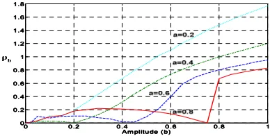
From (19) and (20), the values of ρbhave been plotted in Figure 5. It is seen that ρb gets bigger as the amplitude b increases. However, the increase in ρb gets attenuated as the signal amplitude a increases from 0.2 to 0.8.

0

00

0 0 .20 .20 .20 .2 0 .40 .40 .40 .4 0 .60 .60 .60 .6 0.80.80.80.8 1111

0 0 0 0 0.2 0.2 0.2 0.2 0.4 0.4 0.4 0.4 0.6 0.6 0.6 0.6 0.8 0.8 0.8 0.8 1 1 1 1 1.2 1.2 1.2 1.2 1.4 1.4 1.4 1.4 1.6 1.6 1.6 1.6 1.8 1.8 1.8 1.8

Am plitu de ( b)

Am plitu de ( b)Am plitu de ( b)

Am plitu de ( b)

Figure 5. Variation of ρb versus b for different a amplitudes.

ex(k)

H(z)

yx(k)

+

G(z) Kx

x

(k)

-en(k)

H(z)

+

yn(k)

Kn

Using (18) the quantization noise σ2

qab is plotted in Figure 6. The σ2qab in the regions b < 0.2, b < 0.4 and b < 0.6 for the curves I (a = 0.2), II (a = 0.4) and III (a = 0.6) respectively increases mainly due to ρa. As ρa becomes bigger when the amplitude a increases from 0.2 to 0.6, so does σ2qab. The increase in σ2qab in the regions b > 0.2, b > 0.4 and b > 0.6 for the curves I, II, and III respectively is mainly attributed to the increase in ρb. As

ρb increases with a reduction in the amplitude a from 0.6 to 0.2 in Figure 5, so does σ2

qab.

0 0 0

0 0 .20 .20 .20 .2 0 .40 .40 .40 .4 0.60.60.60.6 0 .80 .80 .80 .8 1111 0 .2

0 .20 .2 0 .2 0 .3 0 .30 .3 0 .3 0 .4 0 .40 .4 0 .4 0 .5 0 .50 .5 0 .5 0 .6 0 .60 .6 0 .6 0 .7 0 .70 .7 0 .7 0 .8 0 .80 .8 0 .8 0 .9 0 .90 .9 0 .9 1 1 1 1

Q

u

a

n

ti

z

a

ti

o

n

N

o

is

e

[image:4.612.328.533.156.281.2]

Signal Amplitude (b)

Figure 6. Variation of quantization noise versus the two sine amplitudes.

Figure 7 shows the noise amplification curves obtained from (40) for a = 0.2, 0.4 and 0.6.

0 0 0

0 0 .20 .20 .20 .2 0 .40 .40 .40 .4 0 .60 .60 .60 .6 0.80.80.80.8 1111 0.5

0.5 0.5 0.5 1 11 1 1.5 1.5 1.5 1.5 2 22 2 2.5 2.5 2.5 2.5 3 33 3

Sign al Am plitu de (b) Sign al Am plitu de (b)Sign al Am plitu de (b) Sign al Am plitu de (b)

N

o

is

e

A

m

p

li

fi

c

a

ti

o

n

A

(K

)

N

o

is

e

A

m

p

li

fi

c

a

ti

o

n

A

(K

)

N

o

is

e

A

m

p

li

fi

c

a

ti

o

n

A

(K

)

N

o

is

e

A

m

p

li

fi

c

a

ti

o

n

A

(K

)

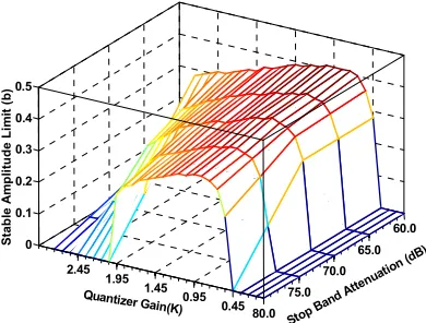
Figure 7. A(k) variation versus the two sine amplitudes. Using the values obtained for Aab(k), the stable amplitude limits for b have been plotted for the 5th- Chebyshev Type II based NTF for a = 0.2 in Figure 8.

0.45 0.95 1.45 1.95 2.45

60.0 65.0 70.0 75.0 80.0 0

0.1 0.2 0.3 0.4 0.5

Stop B and A

ttenu ation

(dB)

Quantizer Ga_in(K)

S

ta

b

le

A

m

p

li

tu

d

e

L

im

it

(

b

)

Figure 8. Stable limits of amplitude b of 5th-order for a = 0.2.

Simulations for the 5th-order Chebyshev Type II based ∆-Σ modulator shown in Figure 9 were performed for 1638400 samples where the input amplitude was increased in steps of 0.1. The maximum stable amplitude limits were obtained and compared with simulations as shown in Figure 9. Results obtained in [3] were used for the DC and single sinusoidal inputs.

d c d cd c

d c s i n es i n es i n es i n e s i n e ( a = 0 . 2 )s i n e ( a = 0 . 2 )s i n e ( a = 0 . 2 )s i n e ( a = 0 . 2 ) s i n e ( a = 0 . 4 )s i n e ( a = 0 . 4 )s i n e ( a = 0 . 4 )s i n e ( a = 0 . 4 ) 0

00 0 0 . 1 0 . 1 0 . 1 0 . 1 0 . 2 0 . 2 0 . 2 0 . 2 0 . 3 0 . 3 0 . 3 0 . 3 0 . 4 0 . 4 0 . 4 0 . 4 0 . 5 0 . 5 0 . 5 0 . 5 0 . 6 0 . 6 0 . 6 0 . 6 0 . 7 0 . 7 0 . 7 0 . 7 0 . 8 0 . 8 0 . 8 0 . 8 0 . 9 0 . 9 0 . 9 0 . 9 1 11 1

S

ta

b

le

A

m

p

li

tu

d

e

L

im

it

(

b

)

S

ta

b

le

A

m

p

li

tu

d

e

L

im

it

(

b

)

S

ta

b

le

A

m

p

li

tu

d

e

L

im

it

(

b

)

S

ta

b

le

A

m

p

li

tu

d

e

L

im

it

(

b

)

[image:4.612.78.273.195.312.2]

P r e d i c t e d P r e d i c t e dP r e d i c t e d P r e d i c t e d S i m u l a t e d S i m u l a t e dS i m u l a t e d S i m u l a t e d

Figure 9. Simulation results for dc, sine & two sinusoidal inputs.

The reason for variation can be attributed to the fact that the derivation of the three gains (i.e. 2 sinusoids and one Gaussian) is based on the modified non-linearity concept. In order to compute the gain for any of the 3 inputs, it is assumed that the non-linear function has been modified in turn by each of the 2 remaining inputs. However, in real-time this may not be the case as all the 3 inputs coexist simultaneously.

V. CONCLUSION

The stability of higher-order ∆-Σ modulators for dual tone sinusoidal inputs using the Describing Function Method has been predicted. The nonlinear gains for the single bit quantizer for a dual sinusoidal input have been derived and the maximum stable input limits for 5th-order Chebyshev Type II based ∆-Σ modulator have been established. Accurate results for the stable amplitude curves can be obtained for a range of values of quantizer gain K in which the ∆-Σ modulators are likely to operate.

APPENDIX A

[image:4.612.79.276.370.487.2] [image:4.612.75.270.551.699.2]

Sinusoidal Gains

The two sinusoidal inputs considered here are xa(t)=aCos(ω1(t)+φ1) and xb(t)=bCos(ω2(t)+φ2) where a, b are constants, ω1, ω2 the sinusoidal frequencies, assumed to be incommensurate, φ1and φ2 are RVs each

having a uniform PDF in the interval [0, 2π]. The second input is the quantization noise assumed to be Gaussian G(0, σ) i.e. with zero mean and variance σ2.The modified nonlinearity of single-bit quantizer with a random input is given by [8]:

_{γ = ∆}

_∫

γ 0 1( ) 2 q(y)dy

n (A1)

where ±∆ is the output of the quantizer and q(y) is the PDF of the random input. Therefore for a Gaussian input:

_∫

_ −

     ∆ =

γ

σ

π σ

γ

0

2 1

2 2

2 1 2 )

( e dy

y

n (A2)

On integration (A2) simplifies to: n₁(γ)

( )

2

σ γ

erf ∆

= (A3)

The non-linearity n1(γ) further modified to n2(γ) by one of the sinusoidal signals say x_a(t) which is given by [7]:

∫

−

+ =

a

a

dx x n x p

n₂(γ) ( ) ₁( γ) (A4)

where p(x) is the PDF of x_a(t). Therefore:

∫

−

      + ∆ − =

a

a

dx x erf x a n

2 1

1 ) (

2 2 2

σ γ π

γ (A5)

n2(γ) is now the nonlinearity of the quantizer which has been modified by the sinusoidal input xa(t) and the quantization noise G(0,σ). The next step is to evaluate the gain for xb(t) to this modified nonlinearity. The gain Kbof the sinusoidal input xb(t) to this non-linearity n2(γ) is given by [8]:

K xn x r xdx

b

b b

b

∫

−

= _σ12 2( ) ( ) (A9)

where σb2= b2/2, is the variance and r(x) the PDF of )

(t

x_b . On integrating (A9) we get the gain Kb for b as:

   

 

+

   

 

−

       

−

           ∆

     

= _{b b}

a

b F

b a

K ρ ψ

ρ σ

π

2 1 1 2 2

1 ₂,

3 , 1 1

2 2 5

(A17)

where,

   

 

+ −

+ −

= ..

6615 128 175

16 45 16 3

4 2 4 6 8

b b

b b

b ρ ρ ρ ρ

ψ (A18)

In order to obtain the gain for xa(t), we proceed as in above to get:

   

 

+    

 

− 

      

−            ∆      

= a a

b

a F

a b

K ρ ψ

ρ σ

π

2 1 1 2 2

1 ₂,

3 , 1 1

2 2 5

(A19)

Noise Gain

The modified nonlinearity of order 1 for a Gaussian input to a single bit quantizer is given by [8]:

∫

∞ ∞ −

      +

= n y H y q y dy

n( , )₁ ( ) ₁ ( )

σ γ γ

σ (A20)

where H1 is the Hermite Polynomial of the first order. Substituting for q(y) and n(y+γ) in (A20):

₂ 2

2 2

2 2

2 2

2 1 ) ,

( σ

γ σ

π π

σ γ

σ −

∞

∞ −

−

∆ _{= ∆}

=

∫

ye dy e

n

y

(A21)

The noise gain Kn in the presence of another random input with PDF p(r) is given by [8]

_∫

∞ ∞ −

= n r p r dr

Kn _σ1 (σ, )1 ( ) (A22) Here we consider the additional random input as a combination of two uncorrelated sinusoidal inputs. The joint PDF p(r) of the two sinusoidal signals having amplitudes a and b, with incommensurate frequencies is: p(r)=(r/πab)(1/sinθ), where θ=cos-1{[a2+b2-r2]/2ab}. Solving the integral above we get the noise gain as:

ζ

σ π

ρ ρ2 2

2 _{a b}

e e Kn

− −

     ∆

= (A27)

where,

   

   

+ + + + +

= ...

576 36 4 1

8 8 6 6 4 4 2

2 a b a b a b

b a

ρ ρ ρ ρ ρ ρ ρ ρ

ζ (A28)

REFERENCES

[1] Risbo, L., “Stability Predictions for Higher-Order Sigma-Delta Modulators Based on Quasilinear Modeling”, IEEE International Symposium on Circuits & Systems, Volume 5, page 361 – 364, 1994.

[2] Gelb, A., Vander Velde, W., E., Multiple-Input Describing Functions and Nonlinear System Design, New York McGraw-Hill, 1968.

[3] Lota, Jaswinder., Al Janabi, Mohammed., Kale, Izzet., “Stability Analysis of Higher-Order Sigma-Delta Modulators using the Describing Function Method”, IEEE International Symposium on Circuits & Systems, Volume 5, page 361 – 364, 2006.

[4] Stikvoort, E., F., “Some Remarks on the Stability and Performance of the Noise Shaper or Sigma-Delta Modulator” IEEE Trans. On Communications, Volume 36, no.10, page 1157-1162, Oct 1988.

[5] Ardalan, S., H., Paulos, J., “An Analysis of Nonlinear Behavior in Delta-Sigma Modulators”, IEEE Transactions on Circuits & Systems,

Volume CAS-34, No.6, June 1987.

[6] Haddad, A., H., Nonlinear Systems, Benchmark Papers in Electrical Engineering and Computer Science, vol. 10, Dowden, Hutchinson & Ross, Inc and Halsted Press, page 197, 1975.

[7] D.P. Atherton, G.F. Turnbull, “Response of Nonlinear Characteristics to Several Inputs and the use of the Modified Linearity Concept in Control Systems”, Proc IEE, vol.111, No.1, pages 157-164, January 1964.

[8] Atherton, D., P., Nonlinear Control Engineering-Describing Function Analysis & Design, Van Notsrand Reinhold London, page 383-388, 1982.