Multiple Representations of Perceptual Features for
Texture Classification and Retrieval
G. Tamilpavai
Assistant ProfessorDepartment of Computer Science and Engineering Government College of Engineering,
Tirunelveli,India
S. Tamil Selvi
PhD. ProfessorDepartment of Electronics and Communication Engineering
National Engineering College, Kovilpatti, India
ABSTRACT
Texture is a very important feature extremely used in various image processing problems. Human beings are used some texture based perceptual features to distinguish between textured images or regions. These Perceptual features are highly desirable for two reasons; they will be optimum in terms of feature selection and will be applicable to all kinds of textures. Some of the important perceptual features are coarseness, contrast, directionality and busyness. This paper proposed a new perception-based approach to content-based image classification and retrieval. The proposal is based on multiple representations: Original Image Representation and Autocorrelation Function Representation. The computational measures for textural features are computed both on original image and autocorrelated image. In order to validate these features measures, applied them for texture classification and retrieval on brodatz images. For texture classification, features computed on Multiple representation correctly classified the best matching class among the existing class in comparison with original representation based features and autocorrelation representation based features. K-Nearest Neighborhood classifier is used for this classification task. For texture retrieval, Multiple representation based features retrieved more number of relevant images in comparison with features derived from autocorrelation representation. Gower co-efficient of similarity is used to find the feature similarity between images in retrieval task. Thus this work attained good classification rate of 93.5% and better retrieval rate by using these estimated features on our approach.
Keywords
Multiple representations, perceptual features, texture, texture classification, texture retrieval.
1.
INTRODUCTION
Texture refers to the spatial distribution of grey-levels and can be defined as the deterministic or random repetition of one or several primitives in an image. Texture feature are widely used for extraction of specific image properties such as coarseness and presence of edges.
A number of texture analysis methods have been proposed [1]-[15]. Haralick [16] categorized texture analysis methods into statistical methods, structural methods, and hybrid methods [17]-[21]. The drawbacks of almost all of these approaches are that they do not have general applicability and computational cost involved, either in terms of memory requirement, computation time or implementational complexity. In comparison, human visual perception seems to work perfectly for almost all types of textures. The reason for
this mismatch between computational methods and human vision is that the majority of the computational methods use mathematical features that have no perceptual meaning. Among the various works that have been done in the field of texture analysis [22], this paper is interested in dealing with human visual perception. In the literature, some works related to perceptual texture analysis have been done [23]-[27]. Tamura et al. [28] and Amadasum et al. [29] proposed, each, computational measures for some textural features such as coarseness, contrast, direction, busyness, regularity and complexity. They studied, then, the correspondence between the classification obtained with these computational measures and classification made by human subjects. The work of Tamura et al. [28] was based on the co-occurrence grey-level matrix (CGLM). The work of Amadasun et al. [29] was based on the neighborhood gray-tone difference matrix (NGTDM). The results they obtained with the computational measures were relatively good with respect to human classification. Ravishankar et al. [30] proposed a texture naming system, i.e. they try to determine the relevant dimensions of texture such as the three dimensional representations of color (RGB, HIS, etc).
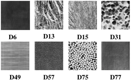
The objective of this paper is to evaluate the computational measures for perceptual textural features. First, proposed a new method to estimate a set of perceptual textural features. Second, application of this proposed perceptual model to texture classification and retrieval task. Our approach is to combine the features which are computed on both original images and the autocorrelation function and applied them for classification and retrieval task to obtain very good classification and retrieval rate. It should be noted that the study reported here was tested on a sample of 8 images (Figure.1) from Brodatz database [31].
Figure 1 shows the block diagram of this work. Autocorrelation function is represented on each input Brodatz image. Computational measures for perceptual textural features are computed both on original image and autocorrelation representation. The feature measures obtained from these two representations are combined and applied for texture classification and retrieval task.
2.
PERCEPTUAL TEXTURAL
FEATURES
In our work, we have considered four perceptual features. In the following, we give conceptual definitions of each of these features.
Coarseness is the most important feature that determines the existence of texture in an image. Coarseness measures the size of the primitives that constitute the texture[32][33]. A coarse texture is composed of large primitives and characterized by a high degree of local uniformity of grey-levels. A fine texture is constituted by small primitives and is characterized by a high degree of local variations of grey-levels.
Directionality is a global property in an image. Directionality measures the degree of visible dominant orientation in an image[34]. An image can have one or several dominant orientation(s) or no orientation at all. In the latter case, it is said isotropic. The orientation is influenced by the shape of primitives as well as by their placement rules.
Contrast measures the degree of clarity with which one can distinguish between different primitives in a texture[35]. A well-contrasted image is an image in which primitives are clearly visible and separable. The contrast is influenced by the grey-levels in the image, the ratio of white and black in the image and the intensity change frequency of grey-levels. Busyness refers to the intensity changes from a pixel to its neighborhood; a busy texture is a texture in which the intensity changes are slow and gradual. Therefore busyness is related to spatial frequency of the intensity changes in an image. If intensity changes are very small, they risk to be invisible. Consequently, the amplitude of the intensity changes has also an influence on busyness. Busyness has a reverse relationship with coarseness.
3.
AUTOCORRELATION FUNCTION
REPRESENTATION
The autocorrelation function of an image can be used to assess the amount of regularity as well as fineness of the texture present in the image, denoted as f(δi, δj). For an n x m image I
is defined as follows[18]:
f
δ
i,δj
=
1
n-δ
i(m-δ
j)
I
i,j
I(i+δ
i, j+δ
j)
m-δj
j=0
n-δi
i=1
(1) where 1 ≤ δi ≤ n and 1 ≤ δj ≤ m. δi and δj represent shift on
rows and columns, respectively.
This function is related to the size of the texture primitive. If the texture is coarse, then the autocorrelation function will drop of slowly; otherwise, it will drop off very rapidly. For regular textures, the autocorrelation function will exhibit peaks and valleys.
4.
COMPUTATIONAL MEASURES FOR
PERCEPTUAL FEATURES
The general estimation process of computational measures simulating human visual perception is as follows[36]-[38].
1) The autocorrelation f( i, j) is computed on image I( i ,j).
2) Then, the convolution of the autocorrelation function and the gradient of the Gaussian function are computed in a separable way (according to rows and columns). Two functions are then obtained.
3) Based on these functions, computational measures for each perceptual features are computed as described in the following subsections.
For multiple representations, the computational measures presented in the following are computed on both the original images and the autocorrelated images.
4.1
Coarseness Estimation
When considering the autocorrelation function, we can notice that coarseness is saved in the corresponding autocorrelation function. Therefore, number of extrema in the autocorrelation function determines coarseness of a texture.
Coarseness, denoted Cs, is estimated as the average number of
maxima in the autocorrelated images and original images. A coarse texture will have a small number of maxima and a fine texture will have a large number of maxima. Coarseness Cs
can be written as
D6
D13
D15
D31
[image:2.595.64.279.71.269.2]D49
D57
D75
D77
Figure 2: Brodatz images used in this work
Input Brodatz
Images
Compute
Autocorrelation
Function
Perceptual
Textural features
Estimation
Application to
Texture Retrieval
Figure 1: Block diagram of proposed system
Application to
[image:2.595.316.537.82.220.2]Cs=
1
0.5 x ( Maxx i,j
m j=1 n i=1
n +
ni=1Maxy i,j
m
j=1
m )
(2)
4.2
Contrast Estimation
If the image is well-contrasted, the value of autocorrelation function decreases quickly; otherwise, it decreases slowly. Therefore, amplitude M of the gradient of the autocorrelation function determines contrast.
Contrast, denoted Ct, is estimated as the product of the
average module Ma of the gradient of the autocorrelation
function, the percentage of points Nt
n x m having a module greater than a threshold t and the coarseness Cs. Coarseness is
introduced here to reflect the fact that a coarse texture is more clearly visible than a fine texture. So contrast is given by
C
t=
M
ax N
tx C
s 1 αn x m
(3)
1
α is a parameter used to make Cs having sense against the
quantity 𝑀ax𝑁t 𝑛x𝑚.
4.3
Direction Estimation
Two parameters are estimated here: the orientation θ and the degree of directionality. The Orientation θ is estimated as the orientation of the gradient of the autocorrelated image or original image. It is given by
θ= arctan G
y/G
x(4) The degree of directionality
𝑁
𝜃𝑑is estimated as the number of points having the dominant orientation θd. The dominantorientation θd is the orientation of the largest number of pixels
in an image having a module greater than a threshold t.
𝑁
𝜃𝑑can be expressed as followN
θd=
ni=1 mj=1
θ
d(i,j)
n x m
(5)
4.4
Busyness Estimation
Busyness is related to coarseness in the reverse order, that is when the coarseness is high, the busyness is low. So busyness is estimated by using coarseness as follow
B
s=1-C
s 1 α(6)
1
αis a parameter used to make Cs having sense against the
quantity 1.
5.
APPLICATION TO TEXTURE
CLASSIFICATION
This experiment was carried out to assess the performance of the perceptual features in texture classification task. Computational features presented in this paper are applied in classification task on Brodatz database. The samples used are D13, D57, D77, D6, D75, D49, D31, and D15. Three kinds of classifications are performed in this work namely original representation based classification, autocorrelation representation based classification and multiple representation based classification. Actual classification task is achieved by K-Nearest Neighborhood classifier.
5.1
K-Nearest Neighborhood classifier
This classifier is used to identify the best matching class among the existing class by using nearest neighbor method. The syntax of knnclassify is defined as followsClass = knnclassify(Sample, Training, Group) (7) Where,
Sample is the matrix whose values represent the set of features which are obtained during testing phase. Sample must have same number of columns as Training.
Training is the matrix whose values represent the set of features which are obtained during training phase.
Group is the vector whose distinct values define different class
5.2
Implementation
Texture classification consist of two phases namely training phase and testing phase. The database contain sample of 8 brodatz images. In training phase, each of these samples is divided into 9 nonoverlapping tiles to obtain 72 subimages of size 128 x 128 (8 images x 9 titles per image). During this phase, leaving out four subimages for each category at a time and training the classifier on the remaining five. Thus, training set and testing set contains 40 (8 images x 5 titles per image) and 32 (8 images x 4 titles per image) subimages respectively. In testing phase, four untrained subimages for each class in the testing set are presented to the classifier to identify the best matching class.
5.3
Classification Based on 9 Subimages
from Each class
5.3.1
Training phase for original representation
Each database image is divided into 9 subimages. Five subimages from each category are stored in training set and remaining goes for testing purpose. Computational measures for perceptual features are computed on training set images. Thus we are obtained the feature set based on original representation.5.3.2
Training phase for autocorrelation
representation
Each database image is divided into 9 subimages. Five subimages from each category are stored in training set and remaining. Autocorrelation function is computed on each image in the training set and perceptual features are estimated. Thus we are obtained the feature set based on autocorrelation representation.
5.3.3
Testing phase for original representation
Perceptual features are estimated on each image in the testing set and obtained the feature set. Knnclassifier is used to find the best matching samples for the testing set images among the existing class in the training set. This is achieved by passing the feature sets which are obtained during training and testing phase for original representation.5.3.4
Testing phase for autocorrelation
representation
5.3.5
Testing phase for multiple representation
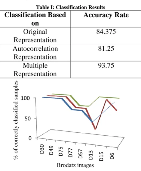
Perceptual features are estimated on each image in the testing set and obtained the feature set on original images. Then, Autocorrelation function is represented on testing set images and features are estimated at a time. Thus obtained the feature set on autocorrelation representation. Knnclassifier is used to find the best matching samples for the testing set images among the existing class in the training set. This is achieved by passing the feature sets which are obtained during training phase for original and autocorrelation representation and testing phase for multiple representations.Classification results are shown in table I. It clearly shows that knnclassifier obtained very good accurate rate in testing phase for multiple representation in comparison with other testing phases. Accuracy rate is defined as follows
Accuracy rate=
𝑇𝑜𝑡𝑎𝑙 𝑛𝑢𝑚𝑏𝑒𝑟 𝑜𝑓 𝑐𝑜𝑟𝑟𝑒𝑐𝑡 𝑚𝑎𝑡𝑐𝑖𝑛𝑔 𝑐𝑙𝑎𝑠𝑠 𝑓𝑜𝑟 𝑡𝑒𝑠𝑡𝑖𝑛𝑔 𝑐𝑙𝑎𝑠𝑠 𝑇𝑜𝑡𝑎𝑙 𝑛𝑢𝑚𝑏𝑒𝑟 𝑜𝑓 𝑠𝑢𝑏𝑖𝑚𝑎𝑔𝑒𝑠 𝑜𝑛 𝑡𝑒𝑠𝑡𝑖𝑛𝑔 𝑠𝑒𝑡
Overall classification performances are shown in figure 3. On these three types of classification, multiple representation based classification shows better accuracy rate in comparison with other two types of classification. It clearly shows that we have obtained more number of correctly classified samples for each category by our approach.
[image:4.595.49.284.375.659.2]5.4
Implementation Result
Table I: Classification Results
Classification Based
on
Accuracy Rate
Original
Representation
84.375
Autocorrelation
Representation
81.25
Multiple
Representation
93.75
Figure 3: Performance measure of texture classification
6.
APPLICATION TO TEXTURE
RETRIEVAL
This experiment was carried out to assess the performance of the features in an actual retrieval task. Computational features presented in this paper are applied in texture retrieval on Brodatz database. The samples used are D13, D57, D77, D6, D75, D49, D31, and D15. Two kinds of retrieval are performed in this work. Retrieval performances are based on the number of subimages derived from each image in the database. Similarity measure used in this work is Gower coefficient of similarity.
6.1
Gower Coefficient of Similarity
The similarity between two texture images GSij, which are
represented by i and j based on all features can be defined as
GSij=
sij (K)
4 k=1
4
(7) Where, sij
(k)
represent the similarity between two images on specific feature k.
Quantity Sij(k) is defined as follows
Sij(k)= 1 −
xik− xjk
Rk
(8) Where, xik is the feature k on given input image
xjk is the feature k on jth image in the database
Rk is the difference between maximum and minimum
value of feature k on feature set X. Quantity Rk is defined as follows
Rk= Max(Xk) – Min(Xk)
(9)
6.2
Implementation
Retrieval task consists of training and testing phase. In training phase, perceptual features are estimated from original image representation and autocorrelation function representation. In testing phase, autocorrelation representation based retrieval and multiple representation based retrieval are carried out.
6.3
Retrieval Based on 9/25 Subimages
from Each class
6.3.1
Training phase for original representation
In the database, each sample is divided into 9/25 subimages of size 128 x 128. Computational measures of perceptual features are estimated from these subimages. Thus obtained the feature set based on original representation.6.3.2
Training phase for autocorrelation
representation
In the database, each sample is divided into 9/25 subimages of size 128 x 128. Autocorrelation function is computed on subimages. Computational measures of perceptual features are estimated from these autocorrelated subimages. Thus obtained the feature set based on autocorrelation representation.
0 50 100
D30 D49 D75
D77 D57 D13
D15 D6
%
o
f
co
rr
ec
tly
class
if
ied
s
am
p
les
Brodatz images
Original representation based classification
Autocorrelation representation based classification
6.3.3
Testing phase for autocorrelation
representation
Autocorrelation function is represented on the image which is given as input. Four features are estimated from this autocorrelated image. Gower coefficient of similarity is measured the similarity between these four features to the feature set which is obtained during the training phase for autocorrelation representation.
6.3.4
Testing phase for multiple representation
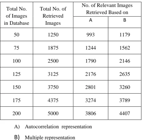
Four perceptual features are estimated from the image which is given as input. On that image, autocorrelation function is represented and four features are computed. Thus eight features are obtained. Similarity measurement is defined between these eight features to the feature sets which are obtained during the training phase for original representation and autocorrelation representation.Retrieval results are shown in tables 1 and table 2. Table 1 shows the retrieval result for 9 subimages from each class. If there n images in the database, then the total number of retrievd images is 9*n. Table 2 shows the retrieval result for 25 subimages from each class. If the total number of images in the database is n, then the total number of retrieved images is 25*n. Retrieval rate is defines as follow,
Retrieval Rate= 𝑁𝑜. 𝑜𝑓 𝑅𝑒𝑙𝑒𝑣𝑎𝑛𝑡 𝑖𝑚𝑎𝑔𝑒𝑠 𝑟𝑒𝑡𝑟𝑖𝑒𝑣𝑒𝑑
𝑇𝑜𝑡𝑎𝑙 𝑛𝑢𝑚𝑏𝑒𝑟 𝑜𝑓 𝑟𝑒𝑡𝑟𝑖𝑒𝑣𝑒𝑑 𝑖𝑚𝑎𝑔𝑒𝑠
Overall retrieval performances are shown in figure 4 and figure 5. In both kind of retrievals, multiple representation based retrieval shows better retrieval rate than autocorrelation based retrieval. It clearly shows that we have retrieved more number of relevant images for our approach.
6.4
Implementation result
Total No. of Images in Database
Total No. of Retrieved
Images
No. of Relevant Images Retrieved Based on
A B
18 162 130 154
27 243 161 197
36 324 222 275
45 405 284 343
54 486 341 410
63 567 422 491
72 648 478 556
A) Autocorrelation representation
B)
Multiple representationTable II: Retrieval result based on 9 subimages from each class
Total No. of Images in Database
Total No. of Retrieved
Images
No. of Relevant Images Retrieved Based on
A B
50 1250 993 1179
75 1875 1244 1562
100 2500 1790 2146
125 3125 2176 2635
150 3750 2801 3260
175 4375 3274 3789
200 5000 3806 4407
[image:5.595.310.548.69.304.2]A) Autocorrelation representation
B)
Multiple representation [image:5.595.307.544.71.729.2]Table III: Retrieval result based on 25 subimages from each class
[image:5.595.48.289.474.713.2]Figure 4: Performance measure of retrieval based on 9 subimages from each class
Figure 5: Performance measure of retrieval based on 25 subimages from each class
0 50 100
18 27 36 45 54 63 72
Re
tri
ev
al
ra
te
Total number of images in the database Autocorrelation representation based retrieval Multiple representation based retrieval
0 50 100
50 75 100 125 150 175 200
Re
tri
ev
al
ra
te
Total number of images in the database Autocorrelation representation based retrieval
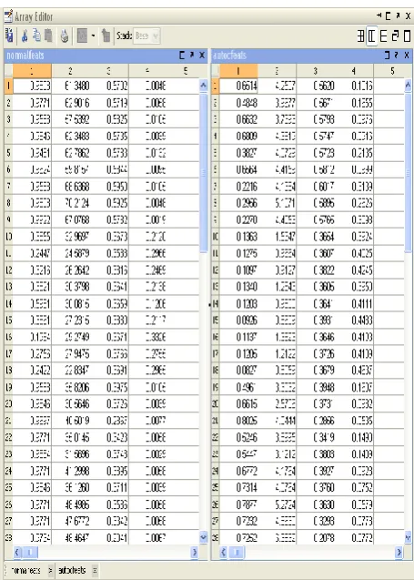
Figure 5: Feature set obtained during training phase for 72 subimages in the database
Figure 6: Feature set obtained during training phase for 200 subimages in the database
7.
CONCLUSION
A new perceptual model based on a set of computational measures corresponding to perceptual textural features namely coarseness, directionality, contrast, and busyness is proposed. Computational measures are based on multiple representations: original image representation and the autocorrelation function associated with original images. Coarseness was estimated as an average of the number of maxima. Contrast was estimated as a combination of the average amplitude of the gradient, the percentage of pixels having the amplitude superior to a certain threshold and coarseness itself. Directionality was estimated as the average number of pixels having the dominant orientation(s). Busyness was estimated based on coarseness. These four basic properties of texture were conceptually defined. The conceptual expressions were put into computational forms. In this approach, autocorrelation function was computed for a given image, and the features were derived from these autocorrelated and original images. In order to validate the proposed set of computational feature measures, applied them in classification and retrieval task on brodatz images. In both applications, better results in terms of classification rate and retrieval rate were obtained by using these developed features based on our approach.
8.
FUTURE WORK
The immediate prospect related to this work is consideration of other perceptual features such as regularity and complexity. Application of these additional computational feature measures with existing features for texture classification and retrieval on large set of images from other texture database.
9.
REFERENCES
[1] R. M. Haralick and L. G. Shapiro, Computer and Robot Vision. Reading, MA: Addison-Wesley, 1992, vol. 1. [2] R. Karu, A. K. Jain, and R. M. Bolle, “Is there any
texture in the image?,” Pattern Recognit., vol. 29, no. 9, pp. 1437–1466, 1996.
[3] J. Zhang and T. Tan, “Brief review of invariant texture analysis methods,” Pattern Recognit., vol. 35, pp. 735– 747, 2002.
[4] A.R. Rao, A Taxonomy for Texture Description and Identification. New York: Springer-Verlag, 1990. [5] M. Galloway, “Texture analysis using gray-level run
lengths,” Computer Graphics Image Processing, vol. 4, pp. 172-199, 1974.
[6] Rosenfeld and M. Thursion, “Edge and curve detection for visual scene analysis,” IEEE Trans. Comput., vol. C-20, pp. 562-569, May 1971.
[7] J. S. Weszka, C. R. Dyer, and A. Rosenfeld, “A comparative study of texture measures for terrain classification,” IEEE Trans. Syst. Man Cybern., vol. SMC-6, pp. 269-285, Apr 1976.
[8] P. C. Chen and T. Pavlidis, “Segmentation by texture using correlation,” IEEE Trans. Pattern Anal. Machine Intell., vol. PAMI-5, pp. 64-69, 1983.
[10] Epifanio.I, Ayala.G, “A random set view of texture classification”, IEEE Trans. Image Process., vol. 11, no. 8, pp. 859-867, Aug 2002.
[11] Zhi-Zong Wang, Jun-Hai Yong, “Texture Analysis and Classification with Linear Regression Model based on Wavelet Transform”, IEEE Trans. Image Process., vol. 17, no. 8, pp. 1421-1430, 2008.
[12] Khellah F.M,” Texture Classification Using Dominant Neighborhood Structure,” IEEE Trans. Image Process., vol. 20, no. 11, pp. 3270-3279, 2011.
[13] Li Liu, Fieguth.P, “ Texture Classification from Random Features”, IEEE Trans. Pattern Anal. Machine Intell., vol.34, no.3, pp. 574-586, 2011.
[14] Xiuwen Liu, Deliang Wang , “ Texture Classification using Spectral Histograms”, IEEE Trans. Image Process., vol. 12, no. 6, pp. 661-670, 2003.
[15] Campisi.p et.al , “ Robust Rotation- Invariant Texture Classification Using a Model Based Approach”, IEEE Trans. Image Process., vol. 13, no. 6, pp. 782-791, 2004. [16] R. M. Haralick, “Statistical and structural approaches to texture,” Proc. IEEE, vol. 67, no. 5, pp. 786–804, May 1979.
[17] R. M. Haralick, K. Shanmugam, and I. Dinstein, “Textural features for image classification,” IEEE Trans. Syst., Man Cybern., vol. 3, no. 6, pp. 610–621, Nov. 1973.
[18] R. Jain, R. Kasturi, and B. G. Schunck, Machine Vision. New York: McGraw-Hill, 1995.
[19] A.H. S. Solberg and A. K. Jain, “Texture analysis of SAR images: a comparative study,” Norwegian Comput. Center and Michigan State Univ., Research Rep., 1997. [20] M. Tuceryan and A. K. Jain, “Texture analysis,” in
Handbook of Pattern Recognition and Computer Vision, C. H. Chen, L. F. Pau, and P. S. P. Wang, Eds. Singapore: World Scientific, 1993.
[21] F. Tomita and S. Tsuji, Computer Analysis of Visual Textures. Norwell, MA: Kluwer, 1990.
[22] L. Van Gool, P. Dewaele, and A. Oosterlinck, “Texture analysis anno 1983,” J. Comput. Vis. Graph. Image Process., vol. 29, pp. 336–357, 1985.
[23] B.Julesz, “Visual pattern discrimination,” IRE Trans., Info. Theory, vol. IT-8, pp. 84092, Feb. 1962.
[24] B. Julesz, E. N Gilbert. L. A. Shepp, and H. L. Frisch. “Inability of humans to discriminate between visual textures that agree in secondorder statistics Revisited.” Perception. vol. 2. pp. 391-405, 1973.
[25] B. Julesz, “Experiments in the visual perception of texture,” Sci. Amer., vol. 232, no. 4, pp. 34–44, 1976. [26] J. R. Bergen and E. H. Adelson, “Early vision and
texture perception,” Nature, vol. 333, no. 6171, pp. 363– 364, May 1988.
[27] Muwei Jian, Lei Liu, Cheng Yin, Lin Yuan, “Combining Perceptual Textural Features and Wavelet Features for Texture Classification”, pp. 238-241, May 2009. [28] H. Tamura, S. Mori, and T. Yamawaki, “Textural
features corresponding to visual perception,” IEEE Trans. Syst., Man Cybern., vol. 8, no. 6, pp. 460–472, Jun. 1978.
[29] M. Amadasun and R. King, “Textural features corresponding to textural properties,” IEEE Trans. Syst., Man Cybern., vol. 19, no. 5, pp. 1264–1274, Sep.-Oct. 1989.
[30] R. Rao and G. L. Lohse, “Towards a texture naming system: Identifying relevant dimensions of texture,” Vis. Res., vol. 36, no. 11, pp. 1649–1669, 1996.
[31] P. Brodatz, Textures: A Photographic Album for Artists and Designers. New York: Dover, 1966.
[32] Rosenfeld and E. B. Troy, "Visual texture analysis," Compt. Sci. Center, Univ. Maryland, College Park, Tech. Rep. TR-1 16, June 1970.
[33] K. C. Hayes, Jr., A. N. Shah, and A. Rosenfeld, "Texture coarseness: Further experiments," IEEE Trans. Syst. Man., Cybern., vol. SMC-4, pp. 467-472, Sept. 1974. [34] R. Bajcsy, "Computer description of textured surfaces,"
in Proc. 3rd Int. Joint Conf. Artificial Intelligence, Aug. 1973, pp. 572-579.
[35] Rosenfeld and A. C. Kak, Digital Picture Processing. New York: L_ Academic, 1976, Chap. 10.
[36] N. Abbadeni, “Computational perceptual features for texture representation and retrieval,” IEEE Trans. Image Process., vol. 20, no. 1, pp. 236-246, Jan 2011.
[37] N. Abbadeni, D. Ziou, and S. Wang, “Computational measures corresponding to perceptual textural features,” in Proc. 7th IEEE Int. Conf.Image Process., Vancouver, Canada, vol. 3, pp. 897–900, 2000.