A Short Term Solution to Implement Applications about Moving Points on Top of Existing DBMSs

A Short Term Solution to Implement Applications about

Moving Points on top of Existing DBMSs

P. Di Felice

Dipartimento di Ingegneria Industriale e dell'Informazione, Economia Università di L'Aquila (Italy)

ABSTRACT

There is an increasing demand for applications about moving objects (e.g., humans, animals, cars, …). The best way to develop robust and efficient software solutions consists in putting them on top of a spatio-temporal database storing the trajectories of the moving objects. Unfortunately, the DataBase Management Systems today part of the companies’ assets do not support this complex data. In this paper, we outline a solution that is feasible in the meantime a new generation of DBMSs will be made available to the community.

General Terms

Databases, trajectory databases, querying, algorithms.

Keywords

Moving points, trajectory databases, spatio-temporal intersection, uncertainty, DBMS, PostgreSQL/PostGIS, SQL.

1.

INTRODUCTION

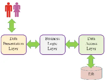
The three–tier client–server architecture is largely adopted to implement complex software applications because it allows to develop and maintain as independent modules (Figure 1) the user interface (Data Presentation Layer), the functional logic (Business Logic Layer), and the access to the data stored into the database server (Data Access Layer). Apart from the usual advantages of modular software with well-defined interfaces, such an architecture allows any of the three tiers to be upgraded independently in response to changes in requirements or technology. In particular, the data access layer isolates the business layer from the details of the specific data storage solution minimizing the impact of changes in the database management system or in the data representation.

Figure 1. Architecture of complex software applications

A relevant category of complex applications is that concerning moving objects. The availability of low cost electronic devices supporting the GPS method is pushing tremendously the software market in such a direction. However, enterprises wish to continue using the assets in operation (among them the DBMSs currently marketed), avoiding new investments both in software and training of its technical staff, particularly in a time of great recession.

Unfortunately, at present are not available mature software technologies to deal with moving objects. The more promising solution at the horizon, namely SECONDO [1], is still in the pipeline. Neither it is easy to use. At the present time SECONDO misses of a stable query optimizer supporting the formulation of SQL scripts both for querying and updating the database. This deficiency drastically reduces the productivity of the developers. In other words, for the time being SECONDO is a good aid both for figures of high expertise and researchers, but it is not suitable to be used in a software factory where workers too often are tight with release deadlines.

In the short period, therefore, the best choice is to procrastinate the use of DBMSs featuring a spatial extender (e.g.: PostgreSQL, IBM-DB2, Oracle) even in the development of spatio-temporal databases on top of which applications about moving objects have to be built. Evidently, however, it will be necessary to add spatio-temporal operators according to the needs posed by the case at hand, drawing on the multiple outcomes that the research has produced over the past ten years in the field of moving objects databases. In essence, the most immediate solution to the problem consists in the realization of a library of functions to be in charge of managing spatio-temporal data.

This article outlines the way to plug this gap by using open-source software (i.e., PostgreSQL/PostGIS). Concretely, as a proof of concept, we implement two efficient and robust operators for moving objects based on an algorithm known in the literature. These operators calculate the solution with linear time in the size of the input (efficiency) making sure that the result “absorbs” the many sources of uncertainty that complicate the solution of problems regarding moving objects (robustness).

In the paper, we concentrate on moving objects for which only the position in space is relevant, therefore abstracted as moving points (for short m-points).

uncertain ones. Sec.6 outlines a real scenario where the adoption of the revised intersection method may be helpful to investigate potential propagation of contagious coming from exposure of m-points to nuclear radiations (a relevant issue, especially after the Fukushima nuclear disaster happened in Japan, for those institutions that are in charge of people health care). Short conclusions end the paper.

2.

NOTATIONS AND DEFINITIONS

In the following, a generic (sharp) trajectory consists of a time ordered sequence of points:

{<P1, t1>,<P2, t2>, …, <Pn+1, tn+1>} (i.e. t1<t2<…<tn+1).

The generic pair of consecutive points PiPi+1 defines a (linear)

line segment over the time interval [ti,ti+1). In turn, a generic

point (Pi) is described by the pair <xi,yi> denoting its

geographic position expressed in a reference system (e.g.: WGS84), while <ti=t(Pi)> is the corresponding timestamp.

The t-value adds semantics to the knowledge of the pure geographic position of the m-point, offering a richer support to the decisions makers.

List of notations used hereinafter: - D: a database of trajectories, - trjA, trjB,…: generic trajectories,

- segi: the i-th line segment of a generic trajectory,

- mpA, mpB, …: the m-points which described the trajectories trjA, trjB, …, respectively,

- from(segi)=ti , to(segi)=ti+1 the functions that applied to

the line segment segi return the timestamps ti, ti+1,

respectively; that is, the initial and the final timestamp in the sense of time.

Let us refer to two generic trajectories (trjA and trjB) of D. A basic test to be carried out is to assess whether trjA and trjB met, and in case they do, compute when and where the rendezvous took place. From a database point of view, to solve this twofold problem requires the availability of two operators (let call them t_meet() and time_meet()) whose formal definition is as follows:

t_meet(): Trj × Trj → {false, true} time_meet(): Trj × Trj → PERIODS

where Trj denotes (with abuse of overloading) the set of all possible trajectories; while PERIODS denotes a set of disjoint time intervals, the i-th of which is the time interval where the i-th spatio-temporal intersection may be occurred.

3.

BACKGROUND

The background about m-points goes back to the pioneer work made by Güting and colleagues [2-4]. In particular, in [5] they introduced the concept of sliced representation, the basic idea of which is to decompose the temporal development of a moving value into a set of temporal units called slices. To each slice is associated a unit defined as the pair {I, f(t)}, where I is a time interval and f(t) is a “simple” function (e.g., linear) that models the movement of the m-point inside I.

Among the many operators they proposed, we concentrate on trajectories intersection whose signature is:

moving(point) ×moving(point) → moving(point), where moving(point) is a data type. In [6] the authors sketched a possible algorithm of such an operator.

In the following, we recall it briefly.

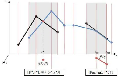
The sequences of units that make up the two trajectories involved in the spatio-temporal intersection are preliminarily synchronized with an operation named refinement partition, which is obtained by breaking the units into other units that have the same value of f(t) but are defined on smaller time intervals, so that a resulting unit of the first argument and one of the second argument are defined either on the same time interval or on two disjoint time intervals. This means that through each point of any segment of both segment sequences, a plane parallel to the x-y-axis is placed obtaining a certain number of slices. As shown in Figure 2, for each slice two situations can happen: either a slice only contains one partial segment from one sequence (white zone) or two partial segments can be found (grey zone). In the former case there can be no intersection. In the latter case the segment intersection test is checked in constant time, using the well-known plane sweep algorithm. If the two segments intersect at the point (x*,y*), then the unit {[t*,t*], f(t)=(x*,y*)} is added to the result, where the interval I coincides with the instant t* in which the m-points occupied the intersection point. If the two segments share a line described by the function f*(t), then the unit {[tini,tend), f*(t)} is added to the result.

Figure 2. A pictorial representation of the intersection

algorithm of two sharp trajectories

Let n and m be the number of consecutive segments of the two sharp trajectories, the computation traverses both sequences until the end of one of them is reached. Each segment is considered exactly once since the time synchronization can be performed on the fly. This leads to a run-time cost of O(n+m).

4.

M-POINTS AND UNCERTAINTY

Working with m-points the following sources of uncertainty come into the picture:

─ uncertainty about the knowledge of the position of the m-points over time. The main sources are: a) uncertainty in the knowledge of the m-point motion law (because of: traffic condition, weather condition, the kind of way on which the movement takes place - city street, provincial road with many bends, mountain road with lots of ups and downs, highway, and the speed limits to take care of); b) measurement errors, c) computational errors, and d) masking of the exact position of the m-points due to privacy/anonymity reasons (e.g., [7]).

─ Uncertainty in the reconstruction of the actual trajectory of the m-points.

m-points, mostly unpredictable in the reality. Studies involving uncertain trajectories are manifold (e.g., [8-11]). Technically speaking, we will implement uncertain trajectories by making recourse to the buffer function.

4.1

From sharp trajectories to uncertain

ones: implications on the intersection

operation

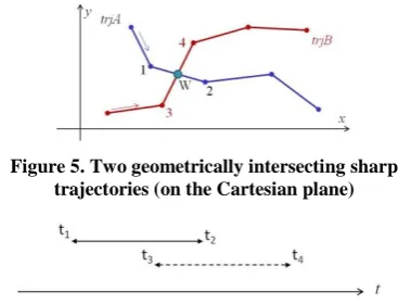
Let segA and segB be the generic line segments of the sharp trajectories trjA and trjB, respectively, between which there exists (by hypothesis) a spatio-temporal intersection. Figure 3 shows such a situation projected on the Cartesian plane: W denotes their rendezvous point. According to the intersection algorithm of Sec.3, W is described by the triple of values <xW,

yW, tW>, claimed to be exact.

Figure 3. Two sharp line segments (projected on the Cartesian plane) in rendezvous (W)

In the following we move from the situation of Figure 3 to that of Figure 4 where the sharp segments (segA and segB), whose geometry is supposed to be exact, are replaced by the corresponding uncertain segments, that is areas centered around the sharp ones.

Figure 4. Two uncertain line segments (on the Cartesian plane) in rendezvous (G)

Consequently, the answer to be returned replaces the point <xW, yW> with the geometry G (Figure 4) and the timestamp

<tW> with the temporal interval:

[max(from(segA), from(segB)), min(to(segA), to(segB))].

Interpretation of G

G denotes the area either crossed by the two m-points in a certain lapse of time or where they stopped for a while. Notice that, pauses visually correspond to line segments parallel to the time axis.

Interpretation of the time interval

To clarify the issue, let us refer to the sharp trajectories of Figure 5. Furthermore, let us assume that the interval [t3..t4] in

which the m-point mpB moved from position 3 to position 4 partially overlaps the interval [t1..t2] in which mpA moved

from 1 to 2 (Figure 6).

If one assume to know the motion law of mpA and mpB when they move from position 1 to 2 and from 3 to 4, respectively, then it is possible to compute if they temporally met in W or not, recurring to some Physics’s law to be embedded into the unit function inside the corresponding interval I. Otherwise,

we cannot state anything. In summary, with regard to Figure 5 and the hypothesis of Figure 6, the answer to the whether issue is “yes”, while the answer to the when issue is expressed in terms of the temporal interval [t3..t2] where such an event

falls, if it happened; circumstance, this latter, not provable analytically any more.

Figure 5. Two geometrically intersecting sharp trajectories (on the Cartesian plane)

Figure 6. The temporal relationship between m-points

mpA and mpB

If we take into consideration the fact that the timestamps linked to the points making up the trajectories to be stored in the database are those for which the m-point position is acquired, it follows that the extent of the interval [t3..t2] is less

or equal to the extent of the acquisition interval. In practical terms, we can say that for most real applications this value is a matter of minutes and, hence, absolutely satisfactory.

5.

THE TIME_MEET ALGORITHM

Below, an algorithm (named time_meet) to calculate the spatio-temporal intersection of pairs of uncertain trajectories is presented as a slight variation of the algorithm sketched in Sec.3. Our algorithm embodies the ideas presented in the previous section. In particular, the uncertain trajectories are obtained by “buffering” the sharp ones stored in the database. ---

Algorithm time_meet (IdTrajA integer, IdTrajB integer, float)

---

Input: IdTrajA, IdTrajB, and (the buffer size)

Output: table result(IdTrajA integer, IdTrajB integer,

intersection_geometry geometry, initial_time timestamp, final_time timestamp)

Method:

1. Let trjA={<A1,t1>, <A2,t2>, …, <An+1,tn+1>} and trjB={<B1,s1>,

<B2,s2>, …, <Bm+1,sm+1>} be the trajectories in the

database identified by idTrajA e idTrajB, respectively. 2. FOR EACH pair {[ti, ti+1), [sj, sj+1)} of overlapping time

intervals detected in a synchronized scan of trjA and trjB DO

3. IF (st_intersects(st_buffer(AiAi+1, ), st_buffer(BjBj+1, ))

THEN

4. geom = st_intersection(st_buffer(AiAi+1, ),

st_buffer(BjBj+1, ))

5. tini = max{ti, sj}

6. tend = min{ti+1, sj+1}

7. Add (IdTrajA, IdTrajB, geom, tini, tend) to the table

result 8. END IF

9. END FOR

10. return result 11. END time_meet

---

Taking advantage of the time ordering of the two trajectories, the time_meet algorithm scans all the pairs of line segments whose intervals temporally overlap (row 2) then, for each pair, it checks (by means of the spatial operators

st_intersection (geometry1, geometry2) - see [12]) whether and where the two participant segments spatially intersect. The first operator (st_intersects())

assesses if it takes place the intersection between two input geometries and returns true in the affirmative case. The second operator, instead, returns a geometry that represents the portion shared between geometry1 and geometry2. Each time the segments spatially intersect the time_meet algorithm first calculates (row 4) the shared intersecting geometry, then it computes (rows 5-6) the temporal window [tini,tend). The spatio-temporal intersection so determined is

added to the result (row 7). The algorithm halts when the end of one of the two trajectories is reached and, hence, all possible pairs {[ti, ti+1), [sj, sj+1)} of overlapping time intervals

have been taken into account.

The algorithm performs all the computations in a single scan of the two trajectories. Since the IF-THEN block of instructions can be executed in constant time (O(1) - the arguments of the st_intersects() and st_intersection() operators are buffered line segments) and the time synchronization can be performed on the fly, the time_meet is executed in O(n+m), where n and m indicate the number of line segments of the two input trajectories.

As final consideration, we note that the intersection algorithm can be easily modified to calculate the intersection test of pair of trajectories, that is, to construct an algorithm (t_meet) that returns true if at least one rendezvous is detected, false otherwise.

6.

A SPATIO-TEMPORAL ANALYSIS

SCENARIO

The algorithm time_meet (as well as t_meet) has been implemented as a User Defined Function called time_meet() (t_meet()) on top of PostgreSQL/ PostGIS. The idea of implementing the two algorithms as UDFs to be added to the built-in UDFs of the system has the double benefit of making them available for being called from any queries as well as from the external software applications that connect to the database.

In this section, we address the need of monitoring the movements of persons (modeled as m-points) in order to detect cases of potential danger of nuclear radiation contagion within known geographic areas. Studies about disease spatial– temporal propagation are supposed to become relevant in the next future (an example may be found in [13]). The merit of the solution sketched below is that it is implemented in terms of scripts that comply with the SQL of the PostgreSQL/PostGIS DBMS.

To manage the reference scenario, it is sufficient to build a database made up of two tables:

radioactiveAreas (ID: integer, Boundary: geometry, DisasterTime: timestamp with time zone ARRAY);

trajectory (Pkey: integer, SSN: varchar(16), Shape: geometry, Confidence: float, TimeValues: timestamp with time zone ARRAY)

The first of them is aimed at the storage of the contaminated areas, while the second collects the trajectories drawn by the m-points. The trajectory geometry has been modeled as a linestring (with linear interpolation between points), while the timestamps of the sampling points are collected in an array of timestamps.

The Confidence attribute stores a float value in the range [0,1]. Let us denote with t the generic tuple in the trajectorytable and let c=t.Confidence. c expresses an evaluation about the “overall quality” of the acquisition process of the geometry of trajectory t. The computation of the extension of the buffer around the trajectory has to be done by taking c into account. In the experiments, we used the simple law: =10/c. Accordingly, the size of “our” buffers ranges from 100 meters (c=0.1) to 10 meters (c=1).

In the following, we implement the query:

“show the SSN of persons that might be infected by the radiations” (Q).

Few general considerations about the problem taken into account follow:

– let us denote with A the set of contaminated areas in the database D (i.e., the tuples in the radioactiveAreas table). In the following, we refer to a single contaminated area called as a;

– let us denote with T the set of trajectories in D (i.e., the tuples in the trajectory table), at a given date. We will assume that all them satisfy the condition that the timestamp of their first point is greater than the value of the attribute DisasterTime of the single tuple in A. In other words, we will assume that all the trajectories in T have been covered after that the nuclear disaster took place in the area a. Such an hypothesis is reasonable in the reality where we can presume that things happen this way: just after a nuclear disaster takes place the Citizens’ Health Care Institute of the country equips itself with the above two-table database. After that, the database will be run as follows:

Step 1: the tuple about area a is inserted in the radioactiveAreas table.

Step 2: the acquisition of the trajectories of the m-points under observation will be started and daily they will be stored in the trajectory table;

– let us denote with T*T the set of trajectories in D that crossed the area a. By construction, T* collects only the contaminated m-points, but unfortunately not necessarily all of them. If trj is the generic trajectory in T*, we call firstCrossTime the instant when, for the first time, the m-point that described the trajectory trj entered the area a. Current DBMSs do not support an operator to the purpose. It is easy to understand that this is a primary need in connection with m-points as attested in [6], where authors proposed the operator:

inside(mp,a):m-point x region → m-bool which returns an m-bool was structure is a time ordered sequence of pairs: <time interval, boolean value> (e.g., <[t1, t2), true>; <[t2, t3), false>; …>). By scanning such a sequence, it is possible to know the time intervals when the m-point mp was inside the input area a. Being available the inside() operator, it is trivial to infer the firstCrossTime value;

To be able to develop the running example, it is sufficient to populate the radioactiveAreas table with a single tuple and the trajectory table with two tuples such that:

– the first tuple concerns a m-point that crossed the area a (and, hence, it is potentially contaminated),

– while the second tuple concerns a m-point that did not enter the contaminated area a, but, for some time, it was nearby the other m-point (after that this latter crossed a) and, hence, it is potentially contaminated as well.

The SQL/DML scripts are listed below:

INSERT INTO radioactiveAreas (ID, Boundary, DisasterTime)

VALUES (22, 'POLYGON(5 5, 11 2, 13 8, 4 8, 5 5)'::GEOMETRY, 2010-10-11 08:00:00)

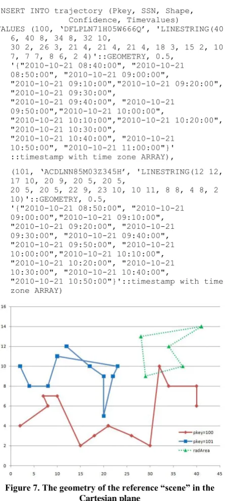
INSERT INTO trajectory (Pkey, SSN, Shape, Confidence, Timevalues)

VALUES (100, ‘DFLPLN71H05W666Q’, 'LINESTRING(40 6, 40 8, 34 8, 32 10,

30 2, 26 3, 21 4, 21 4, 21 4, 18 3, 15 2, 10 7, 7 7, 8 6, 2 4)'::GEOMETRY, 0.5,

'{"2010-10-21 08:40:00", "2010-10-21 08:50:00", "2010-10-21 09:00:00",

"2010-10-21 09:10:00","2010-10-21 09:20:00", "2010-10-21 09:30:00",

"2010-10-21 09:40:00", "2010-10-21 09:50:00","2010-10-21 10:00:00",

"2010-10-21 10:10:00","2010-10-21 10:20:00", "2010-10-21 10:30:00",

"2010-10-21 10:40:00", "2010-10-21 10:50:00", "2010-10-21 11:00:00"}' ::timestamp with time zone ARRAY),

(101, ‘ACDLNN85M03Z345H’, 'LINESTRING(12 12, 17 10, 20 9, 20 5, 20 5,

20 5, 20 5, 22 9, 23 10, 10 11, 8 8, 4 8, 2 10)'::GEOMETRY, 0.5,

'{"2010-10-21 08:50:00", "2010-10-21 09:00:00","2010-10-21 09:10:00", "2010-10-21 09:20:00", "2010-10-21 09:30:00", "2010-10-21 09:40:00", "2010-10-21 09:50:00", "2010-10-21 10:00:00","2010-10-21 10:10:00", "2010-10-21 10:20:00", "2010-10-21 10:30:00", "2010-10-21 10:40:00",

"2010-10-21 10:50:00"}'::timestamp with time zone ARRAY)

Figure 7. The geometry of the reference “scene” in the Cartesian plane

Figure 7 shows the geometry of “the scene” (projected on the x-y Cartesian plane) that reflects the content of the example

database we refer to in this section. Figure 8 shows the two sharp trajectories in the 2D+t space.

6.1

Implementation of query

Q

Aim of Q is to compute the set T*T**. The result is obtained by combining the tuples about the m-points that crossed the contaminated area a (i.e., the set T*) and the tuples concerning the m-points that came in contact with the first ones after that they became contaminated (T**). The general formulation of Q follows.

Figure 8. The two sharp trajectories in 2D + time

SELECT DISTINCT t.SSN – – the set T*

FROM trajectory AS t, radioactiveAreas AS a WHERE st_intersects(t.Shape, a.Boundary) AND

id=22

UNION

SELECT DISTINCT t1.SSN – – the set T**

FROM trajectory AS t1, trajectory AS t2 WHERE t_meet(t1.Pkey,t2.Pkey,20) = true

AND t1.Pkey<>t2.Pkey

AND t1.Pkey NOT IN – – (t1 does not belong to T*)

(SELECT t.Pkey

FROM trajectory AS t, radioactiveAreas AS a

WHERE st_intersects(t.Shape, a.Boundary) AND id=22)

AND t2.Pkey IN – – (t2belongs to T*)

(SELECT t.Pkey

FROM trajectory AS t, radioactiveAreas AS a

WHERE st_intersects(t.Shape, a.Boundary) AND id=22)

AND “at least one rendezvous occurred between t1 and t2, after that t2 entered area a”

Query Q, though long, is almost trivial apart from the computation of the last AND condition which implies to make recourse to the time_meet() operator within a PL/pgSQL code necessary to compensate for the lack of spatio-temporal operators on such an implementation platform (as well as in the others DBMSs on the market). As it was anticipated, what we need is the inside(mp,a) operator to which the computation of the firstCrossTime timestamp for the m-point (mp) that entered the contaminated area a should be hooked.

Figure 9 shows the SQL reformulation of query Q according to our example and its output as well.

Figure 9. Q and its output

To give evidence that the trajectories Pkey=100 and Pkey=101 actually met after that the first one crossed the contaminated area a, it is sufficient to make recourse to the following simple query:

SELECT time_meet(100, 101, 20).

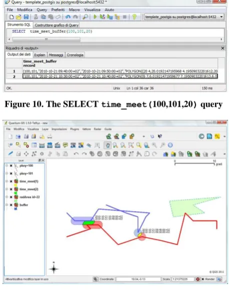
This way, we have also the chance to show how the output of the time_meet() operator looks like both in textual form (Figure 10) and graphically (Figure 11 and Figure 12).

Figure 10. The SELECT time_meet(100,101,20) query

Figure 11. QGIS visualization of the query SELECT time_meet(100,101,20)

The QGIS [14] screen of Figure 11 is very helpful because it shows graphically the geometry of the two trajectories projected on the x-y Cartesian plane and the rendezvous between those two trajectories. The rendezvous (visualized as

a circle) corresponds to a stop point for the two m-points (as it becomes clear by looking at Figure 8).

Figure 12, which is alternative to Figure 11, has the further merit of making explicit that the time_meet() (t_meet()) operator uses uncertain trajectories in the computation of the spatio-temporal intersection.

Figure 12. A visualization alternative to that of Figure 11

7.

CONCLUSIONS

In this paper, we outlined a way to give an answer to the large expectations of enterprises to start up their own software applications about historical trajectories on top of the DBMSs they are equipped with.

On the technological side, the open-source system PostgreSQL/PostGIS would be a great solution, obviously either IBM-DB2/SE or Oracle Spatial are equally good.

On the methodological side, the work to be done consists in the implementation of ad hoc operators as required by the application at hand. In the paper, as a proof of concept, we took into account the spatio-temporal intersection of pairs of trajectories. The happy note comes from the literature about the m-points that offers a reach variety of algorithms to refer to.

8.

REFERENCES

[1] Güting, R.H., Behr, T., and Düntgen, C. 2010. SECONDO: A platform for moving objects database research and for publishing and integrating research implementations. IEEE Data Engineering Bulletin 33:2, 56-63.

[2] Erwig, M., Güting, R.H., Schneider, M., and Vazirgiannis, M. 1999. Spatio-Temporal Data Types: An Approach to Modeling and Querying Moving Objects in Databases. GeoInformatica 3, 265-291.

[3] Güting, R. H., Bohlen, M. H., Erwig, M., Jensen, C. S., Lorentzos, N. A., Schneider, M., and Vazirgiannis, M. 2000. A foundation for representing and querying moving objects. ACM Transactions on Database Systems, 25(1), 1-42.

[4] Güting, R.H. and Schneider M. 2005. Moving Objects Databases. Morgan Kaufmann Publishers.

[6] Cotelo Lema, J.A., Forlizzi, L., Güting, R. H., Nardelli, E., and Schneider, M. 2003. Algorithms for Moving Object Databases. The Computer Journal, 46(6), 680-712.

[7] Giannotti, F. and Pedreschi, D. 2008. Mobility, Data Mining and Privacy. Springer.

[8] Trajcevsky, G., Wolfson, O., Hinrichs, K., and Chamberlain, S. 2004. Managing uncertainty in moving object databases. ACM Transactions on Database Systems, 29(3), 463-587.

[9] Abul, O., Bonchi, F., and Nanni, M. 2008. Never walk alone: uncertainty for anonymity in Moving Object Databases. In Proc. of the 24th International Conference on Data Engineering.

[10] Frentzos, E., Gratsias, K., and Theodoridis, Y. 2009. On the Effect of Location Uncertainty in Spatial Querying.

IEEE Transactions on Knowledge and Data Engineering, 21(3).

[11] Kuijpers B. and Othman W. 2010. Trajectory databases: Data models, uncertainty and complete query languages. Journal of Computer and System Sciences. 76(7), 538-560.

[12] OpenGIS Implementation standard for geographic information. 2007. Simple feature Access, Part 2: SQL Option (ref. number: OGC 06-104r4).