The Adomian Decomposition Method and the Differential Transform Method for Numerical Solution of Multi Pantograph Delay Differential Equations

(1)

http://dx.doi.org/10.4236/am.2015.68126

The Adomian Decomposition Method and

the Differential Transform Method for

Numerical Solution of Multi-Pantograph

Delay Differential Equations

Musa Cakir, Derya Arslan

Department of Mathematics, Faculty of Science, University of Yuzuncu Yil, Van, Turkey Email: cakirmusa@hotmail.com, ayredlanu@gmail.com

This work is licensed under the Creative Commons Attribution International License (CC BY).

http://creativecommons.org/licenses/by/4.0/

Abstract

In this paper, the Adomian Decomposition Method (ADM) and the Differential Transform Method (DTM) are applied to solve the multi-pantograph delay equations. The sufficient conditions are given to assure the convergence of these methods. Several examples are presented to demonstrate the efficiency and reliability of the ADM and the DTM; numerical results are discussed, compared with exact solution. The results of the ADM and the DTM show its better performance than others. These methods give the desired accurate results only in a few terms and in a series form of the so-lution. The approach is simple and effective. These methods are used to solve many linear and nonlinear problems and reduce the size of computational work.

Keywords

Multi-Pantograph Delay Differential Equations, Adomian Decomposition Method (ADM), Differential Transform Method (DTM), Convergence of Adomian Decomposition Method

1. Introduction

(2)

In recent years, the multi-pantograph delay differential equations were studied by many authors. For examples, Li and Liu [2] applied the Runge-Kutta methods to the multi-pantograph delay equation. Evans and Raslan [3]

used the Adomian decomposition method for solving the delay differential equation. Keskin et al. [4] applied the differential transform method to obtain the approximate solution. Sezer and Dascioglu [5] developed and ap-plied the Taylor method to the generalized pantograph equation with retarded case or advanced case. Brunner [1]

used the collocation methods for pantograph-type Volterra functional equations with multiple delays. Yu [6] ap-plied the variational iteration method to the multi-pantograph delay equation. Sezer et al. [7] worked approximate solution of multi-pantograph equation with variable coefficients. Geng, F. Z. and Qian, S. P. [8] worked the Reprociding Kernel Medhod to Solving Singularly Perturbed Multi-Pantograph Delay Equations. Cherruault, Y., Adomian, G., Abbaoui, K. and Rach, R. [9] worked on Convergence of Decomposition Method. Ismail et al. [10]

gave the numerical solutions of the Korteweg-De-Vries (KDV) and modified Korteweg-De-Vries Equations. El-Safty et al. [11] studied on the 3-h step spline function approximation to the solution of delay dynamic sys-tem. Saeed and Rahman [12] established the differential transform method to solve systems of linear or non-linear delay differential equation.

A numerical method based on the Adomian Decomposition Method (ADM) which has been used from the 1970s to the 1990s by George Adomian [13] [14]. The differential transform method (DTM) has been success-fully developed by Zhou (1986) in electric circuit analysis. DTM has been used to solve linear and nonlinear differential equations [15].

ADM and DTM have been shown to solve effectively, easily and accurately a large class of linear and nonli-near, ordinary, partial, deterministic or stochastic differential equations with approximate solutions which con-verge rapidly to accurate solutions [3] [4] [13] [14]. The basic motivation of this work is to apply the ADM and DTM to the DDE. It is well known now in the literature that this algorithm provides the solution in a rapidly convergent series [3] [4]. ADM and DTM are very effective and convenient for solving multi-pantograph equa-tions [3] [4].

This study is presented as follows: In second section, we start by presenting ADM and DTM to solve mul-ti-pantograph delay differential equations. In third section, we continue to the presentation of the convergence of ADM with Theorem 3.1 and Definition 3.2. In fourth section, these methods are shown and compared by four examples by taking various values for t and error evaluation is made. Also, we have plotted the graphs for nu-merical solutions of ADM and DTM and exact solution.

We examined that multi-pantograph delay differential equations are solved by several methods. Thus, we wanted to show up that may be more efficient, simpler and reliable the solution treatment of the ADM for multi- pantograph delay differential equations. The results show that the ADM is more powerful method than other methods for multi-pantograph delay differential equations.

2. Analysis of Adomian Decomposition Method and the Differential Transform

In this paper, we consider the following multi-pantograph equations [16],

( )

( ) ( )

( )

1

, 0 k

i i

i

y t a t y t b t y q t f t t T

=

′ = +

_∑

+ ≤ < (1)

( )

0,

y t =y (2)

( ) ( ) ( )

, i ,

a t b t f t are analytical functions, 0<qi<1,i=1,,k. Using the ADM, the differential operator L is given by

( )

d

( )

. .

d n

n

L t

= (3)

The inverse operator L−1, this is n-fold integral operator defined by

( )

1

-times 0

. t ._n d

L− =

∫

t (4)

operating with L−1 on Equation (1), it then follows

(3)

where the method defines Ny the nonlinear term by the Adomian polynomials [3] [13] [14] 0 , n n Ny A ∞ = =

∑

n

A are Adomian polynomials that can be generated for all forms of nonlinearity as

1 ₀ 1 d , ! d n n i

n n i

i

A N y

n α =α _α₌

  

= _ _ __

 



∑



where i=0,1, 2,3,

( )

0 0

A = f y

( )

1 1 0

0 d d

A y f y

y

 

=  

 

( )

12 2

( )

2 2 0 2 0

0

d d

d 2! d

y

A y f y f y

y y

    

= _ _ +_ _ _

  

 

( )

2

( )

13 3

( )

3 3 0 1 2 2 0 3 0

0 0 0

d d d

.

d d 3! d

y

A y f y y y f y f y

y y y

      

=   +   +  

 

     

Operating with L−1 on Equation (5), it then follows

1 1 1 1

L Ly− +L Ry− +L Ny− =L f− (6)

( )

1 1 1

0

y=y +L f− −L Ry− −L Ny− (7)

1 1 1

0

0 n 0 n 0 n

n y y L f L R n y L n A

∞ − − ∞ − ∞

= = + − = − =

∑

(8)

to determine the components

( )

, 0. n

y t n≥

First, we identify the zero component y t₀

( )

by all terms that arise from the boundary conditions at t = 0 and from integrating the source term if it exists. Second, the remaining components of y t

( )

can be determined in a way such that each component is determined by using the preceding components [3] [13] [14]

( )

1

0 0 ,

y =y +L f− (9)

and Equation (8) gives for n=1, 2,3, in other words, the method introduces the recursive relation

1 1

1 0 0

1 1

2 1 1

1 1

3 2 2

1 1

1

n n n

y L Ry L A

− − − − − − − − + = − − = − − = − − = − −  (10)

The Adomian decomposition method assumes that the unknown function y t

( )

can be expressed by an infi-nite series of the form [3] [13] [14]

( )

0 1 2

0 n n

y t y y y y

∞

=

∑

= + + +

so that the components y t_n

( )

will be determined recursively [3] [13] [14]

Differential Transform Method

(4)

( )

0 d 1 ! d k k x y x Y k

k x ₌

 

= _ _

 

  (11)

In Equation (11), y x

( )

is original function and Y k

( )

is the transformed function, which is called the T- function. Differential inverse transform of Y k

( )

is defined as

( )

0 k

k

Y k x Y k

∞

=

∑

(12)

From Equations (12) and (11), we obtain

( )

0

( )

0 d ! d k k k k x y x x y x k x ∞ = =   =      

∑

(13)

Equation (13) implies that concept of differential transform is derived from Taylor series expansion, but the method does not evaluate the derivatives symbolically.

In actual applications, the function y x

( )

is expressed by the a finite series and Equation (12) can be written as

( )

0

( )

m k

k

y x =

∑

₌ x Y k (14)

Equation (13) implies that is

( )

1 k

k m

y x x Y k

∞

= +

=

∑

is negligibly small. In fact, m is decided by the convergence of natural frequency in this study.

The following theorems that can be deduced from Equations (11) and (12) are given below, see [17] [18].

Theorem 1 If y t

( )

=g t

( ) ( )

+h t , then Y k

( )

=G k

( )

+H k

( )

.

( )

=cg t

( )

, then Y k

( )

=cG k

( )

.

Theorem 3 If

( )

d

( )

d k

k

g t

y t = , then

( ) (

) ( )

!

k n

Y k G k n

k

+

= + .

( )

=g t

(

+a

)

, then

( )

N h k

( )

m k

h

Y k a G m

k − =   = _{ }  

∑

, for N→ ∞.

( )

g t a 1

a

  = _{ } ≥

  , then

( )

( ) (

)

0

( )

1

1 , for .

h k N

h k h k h k

h h k

h a

Y k t a G h N

k a − − − − = −   = − _{ } → ∞  

∑

3. The Convergence of ADM

The Adomian Decomposition Method is equivalent to the sequence defined as follows [19] [20]

1 2 3 ,

n n

S = y +y +y + + y

by using the iterative scheme

(

)

0 1 0 0, n n S

S+ N y S

=

= + (15)

and related to the functional equation

(

0

)

.

S=N y +S

The numerical solution of Equation (15) was used fixed-point theorem by Cherruault [19] [20].

Theorem 3.1 Let N be an operator from Hilbert space H in to H and y be the exact solution of functional equ-ation.

0 i i y

∞ =

(5)

{ }

0

k N

∀ ∈  .

Proof See [19] [20].

Definition 3.2 For every i∈N

{ }

0 we define

1

, 0,

0, 0,

i i i i

i y

y y

y

α

+



≠ 

= 

 ₌



Corollary 3.3 In Theorem 4.1,

0 i i y

∞ =

∑

converges to exact solution y, when 0≤αi<1,i=1, 2,3,

4. Numerical Examples

In this section, four experiments of multi-pantograph delay differential equations are given to illustrate the effi-ciency of the ADM and the DTM. The examples are computed using Maple 15. Results obtained by the methods are compared with the exact solution of each example and found to be good agreement with each other. The ab-solute errors in tables are given at selected points.

Example 4.1 Consider the following linear multi-pantograph delay equation of the first-order [16]

( )

2

5

4 9 1, 0 1,

6 2 3

0 1,

t t

y t y t y y t t

y

   

′ = − + _{ }+ _{ }+ − < ≤

   

=

which has the exact solution,

( )

₁ 67 1675 2 12157 3_.

6 72 1296

y t = + t+ t + t

Using the ADM, we get according to Equations (3)-(10), we obtain recursive formula for k=0,1, 2,3,,

( )

1 1

5

4 9

6 2 3

k k k k

t t

y₊ =L− _− y t + y _{ } + y  _{ }_

   

 

3 0

1 1

3

y = + t −t

2 1

73 25

6 12

y = t− t

2 3

2

1825 175

72 216

y = t − t

3 3

12775

1296

y = t

Thus, we obtain

( )

2 3

ADM 0

67 1675 12157

1 0 0

6 72 1296

n n

y t y t t t

∞

=

∑

= + + + + + +

The solution by DTM method:

By using Theorems of DTM, we have following recurrence relation:

(

)

( )

5 4 9

(

) ( )

( )

1 2 , 1, 0 1

1 6 2k 3k

Y k

Y k k k k Y

k δ δ

 

+ = _− + + _+ − − ≥ =

+  

(6)

( )

67

( )

1675

( )

12157

( )

1 , 2 , 3 , 4 0, 5 0,

6 72 1296

Y = Y = Y = Y = Y = 

Finally, the differential inverse transform of Y k

( )

gives

( )

0 k

k

y t Y k t

∞

= =

∑

we obtain the following series solution

( )

2 3

DTM

0

67 1675 12157

1 0 0

6 72 1296

k

y t Y k t t t t

∞

=

∑

= + + + + + +_

the closed form of above solution is

( )

₁ 67 1675 2 12157 3

6 72 1296

y t = + t+ t + t

which is exactly the same as the exact solution.

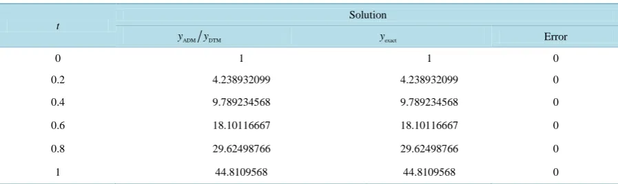
The obtained results (ADM and DTM) are exactly the same with the one found by exact solution. It is clear from Table 1 and Figure 1 that the three results not only give rapidly convergent series but also accurately compute the solutions.

[image:6.595.83.424.81.259.2]

Using our methods, we choose 6 points on [0, 1] respectively. The numerical results are given in the following Table 1.

Example 4.2 Solve the following nonlinear pantograph delay equation of first-order [3]

( )

2

1 2 , 0 1

2

0 0,

t

y t y t

y

 

′ = − _{ } ≤ ≤

  =

which has the exact solution, y t

( )

=sin .t

The solution by ADM method:

By applying the ADM, according to Equations (3)-(10), we obtain

2 1 2

2

t Ly= − y  _{ }

 

( )

1 1 2 1

2 1

2

t L Ly− =L− _− y  _{ }_+L−

 

( )

1 2

2 2

t y t =L− _− y  _{ }_+t

 

[image:6.595.134.491.438.695.2]

 

Figure 1. The obtained solution of the multi-pantograph delay equation [ADM solution (red), DTM

(7)

[image:7.595.87.536.99.233.2]

Table 1. Comparison of exact solution, the (ADM) and the (DTM) of y(t).

t

Solution

ADM DTM

y y yexact Error

0 1 1 0

0.2 4.238932099 4.238932099 0

0.4 9.789234568 9.789234568 0

0.6 18.10116667 18.10116667 0

0.8 29.62498766 29.62498766 0

1 44.8109568 44.8109568 0

We have solved this problem using the proposed method. Recursive formula and the sequence of approximate solution are obtained as follows:

( )

1 2

2

k k

t y₊ t = −L− _ y  _{ }_

 

3

1 0, ( )

6

t k= y t = −

( )

5 7

2 3

1, , 2, ( )

120 5040

t t

k= y t = k= y t = −

thus, we obtain:

( )

3 5 7

ADM

0 3! 5! 7!

n n

t t t

y t y t

∞

=

∑

= − + − +_

Using to convergence of ADM’s method,

1 _{, 0} _1, _{0,1, 2,3,} _. i

i i

i

y

i y

α ₌ + _≤α _< ₌ _

0

1

2

0.5000000000 1 0.02380952381 1

0.01302729713 1 α

α α

= <



Here, the values of α_i are less than one and hence ADM is convergent. The solution by DTM method:

(

) (

)

( )

( ) (

)

( )

0

1 1 2 , 1, 0 1

k

r

k Y k δ k Y r Y k r k Y

=

+ + = −

∑

− ≥ =

Utilizing the recurrence relation, we find

( )

1

( )

1

1 1, 2 0, 3 , 4 0, 5 ,

3! 5!

Y = Y = Y = − Y = Y = 

( )

gives

( )

0 k

k

y t Y k t

∞

= =

_∑

(8)

( )

3 5 7

DTM

3! 5! 7!

t t t

y t = − + − +t 

The obtained results (ADM and DTM) are exactly the same with each other. Increasing the approximation order up to the absolute differences between the numerical solutions are calculated for and comparisons have been made with known results as reported in Table 2 and Figure 2.

Example 4.3 Consider the following linear multi-pantograph delay equation of the first-order [21].

( )

(

) (

)

( )

3 0.4 0.4 0.1 , 0 1,

0 2.127,

y t y t y t y t t

y

′ = − + + < ≤

=

( )

(

) ( )

3 0.4 0.4 0.1

Ly= − y t + y t +y t

( )

(

) (

)

(

)

1 1

3 0.4 0.4 0.1

L Ly− =L− − y t + y t +u t

( )

1

(

( ) (

) (

)

2.127 3 0.4 0.1

y t = −L− y t −y t −y t

( )

(

)

(

)

(

)

1

1 3 0.4 0.4 0.1

k k k k

[image:8.595.93.535.364.521.2]

y₊ =L− − y t + y t +y t

Figure 2. The obtained solution of the multi-pantograph delay equation [ADM solution (red), DTM solution (blue), EXACT

solution (black)].

Table 2. Comparison of the ADM, the DTM and the EXACT solution.

t

Solution

ADM

y yDTM yEXACT

0 0 0 0

0.2 0.198669331 0.198669 0.198669333

0.4 0.389418342 0.389418 0.389418342

0.6 0.564642446 0.564642 0.564642446

0.8 0.717355723 0.717356 0.717355723

[image:8.595.89.535.575.718.2]

(9)

0 2.127,

y =

1

0, 3.403200000

k= y = − t

2 2

1, 4.662384000

k= y = t

3 3

2, 4.547378527

k= y = − t

4 4

3, 3.380293828

k= y = t

Thus, we obtain:

( )

2 3 4

ADM 2.127 3.403200000 4.662384000 4.547378527 3.380293828

y t = − t+ t − t + t −

The solution by DTM method:

(

)

( )

2 1 1

( )

1 3 , 1, 0 2.127

1 5 10

k

k Y k

Y k k Y

k

+

 _{ } 

+ = − +_{ } +  ≥ =

+    

Using the recurrence relation, we find

( )

1 3.403200000, 2 4.662384000, 3 4.547378528,

4 3.380293829, 5 2.021185850,

Y Y Y

Y Y

= − = = −

= = − 

( )

gives

( )

0 k

k

y t Y k t

∞

= =

_∑

( )

2 3 4 5

2.127 3.403200000 4.662384000 4.547378528 3.380293829 2.021185850

y t = − t+ t − t + t − t +

The obtained results (ADM and DTM) are exactly the same with the one found by exact solution. It is clear from Table 3 and Figure 3 that the two results not only give rapidly convergent series but also accurately com-pute the solutions.

Example 4.4 Consider the following linear multi-pantograph delay equation of the first-order [21].

( )

(

)

(

)

( )

0.8 0.5 0.1 0.25 , 0 1,

0 1,

y t y t y t y t t

y

′ = − − + < ≤

=

( )

0.8

(

0.5

)

0.1

(

0.25

)

Ly= −y t − y t + y t

( )

(

)

(

)

(

)

1

0.8 0.5 0.1 0.25

Ly=L− −y t + y t + u t

( )

1

(

( )

(

)

(

)

1 0.8 0.5 0.1 0.25

y t = −L− y t + y t − y t

( )

(

)

(

)

(

)

1

1 0.8 0.5 0.1 0.25

k k k k

y₊ =L− −y t + y t + y t

( )

0 1, 0 1,

y = y =

1

0, 1.700000000

k= y = − t

2 2

1, 1.68750000

(10)

[image:10.595.83.538.82.257.2]

Figure 3. The obtained solution of the multi-pantograph delay equation [ADM solution (red), DTM solution (blue)].

Table 3. Comparison of the ADM solution yADM with the solution by DTM is illustrated.

t

Solution

ADM

y y_DTM

0 2.127 2.127

0.2 1.601884802 1.601884802

0.4 1.307204736 1.307204736

0.6 1.219390558 1.219390558

0.8 1.444676306 1.444676306

1 2.219099301 2.219099301

3 3

2, 0.4650651040

k= y = − t

4 4

3, 0.1277112376

k= y = t

Thus, we obtain:

( )

2 3

ADM

0

1 1.700000000 1.68750000 0.4650651040 n

n

y t y t t t

∞

=

_∑

= − + − +_

Using to convergence of ADM’s method,

1

, 0 1, 0,1, 2,3, . i

i i

i

y

i y

α ₌ + _≤α _< ₌ _

0

1

2

0.9926470588 1 0.2755941357 1 0.2746093751 1 α

α α

= <



according to the obtained results ADM is convergent to the exact solution. The solution by DTM method:

[image:10.595.86.538.304.456.2]

(11)

(

)

( )

0.8 0.1

( )

1 1 , 1, 0 1

1 2k 4k

Y k

Y k k Y

k

 

+ = _− + + _ ≥ =

+  

Utilizing the recurrence relation, we find

( )

1 1.7,

( )

2 1.168750000 ,

( )

3 0.4650651042,

( )

4 0.127712376,

Y = − Y = t Y = − Y = 

( )

gives

( )

0 k

k

y t Y k t

∞

= =

_∑

( )

2 3 4

1 1.7 1.168750000 0.4650651042 0.127712376

y t = − t+ t − t + t −

The obtained results (ADM and DTM) are exactly the same with the one found by exact solution. It is clear from Table 4 and Figure 4 that the two results not only give rapidly convergent series but also accurately com-pute the solutions.

5. Conclusion

[image:11.595.91.527.393.541.2]

It has been the aim of this paper to show that it appears natural to approximate the solution of multi-pantograph delay differential equation by ADM and DTM. We obtain the high approximate solutions or the exact solutions within a few iterations. It is concluded from figures and tables that the successive approximations methods are an accurate and efficient method to solve multi-pantograph delay differential equations. Some numerical exam-ples have been provided to illustrate that the present method is effective in accuracy and convergence speed. In a word, the ADM and DTM show that the techniques are reliable, powerful and promising methods for linear

Figure 4. The obtained solution of the multi-pantograph delay equation [ADM solution (red), DTM solution (blue)].

Table 4. Comparison of the ADM solution y_ADM with the solution by DTM is illustrated.

t

Solution

ADM

y yDTM

0.0 1 1

0.2 0.703233817 0.703233817

0.4 0.480505241 0.480505241

0.6 0.316847313 0.316847313

0.8 0.202197189 0.202197189

[image:11.595.88.538.585.721.2]

(12)

and nonlinear problems.

References

[1] Ockendon, J.R. and Taylor, A.B. (1971) The Dynamics of a Current Collection System for an Electric Locomotive.

Proceedings of the Royal Society of London A, 322, 447-468. http://dx.doi.org/10.1098/rspa.1971.0078

[2] Li, D. and Liu, M. (2005) Runge-Kutta Methods for the Multi-pantograph Delay Equation. Applied Mathematics and Computation, 163, 383-395. http://dx.doi.org/10.1016/j.amc.2004.02.013

[3] Evans, D.J. and Raslan, K.R. (2005) The Adomian Decomposition Method for Solving Delay Differential Equation.

International Journal of Computer Mathematics, 82, 49-54. http://dx.doi.org/10.1080/00207160412331286815 [4] Keskin, Y., at al. (2007) Approximate Solutions of Generalized Pantograph Equations by the Differential Transform

Method. International Journal of Nonlinear Sciences and Numerical, 8, 159-164.

http://dx.doi.org/10.1515/IJNSNS.20078.2.159

[5] Sezer, M. and Dascioglu, A.A. (2007) A Taylor Method for Numerical Solution of Generalized Pantograph Equations with Linear Functional Argument. Journal of Computational and Applied Mathematics, 200, 217-225.

http://dx.doi.org/10.1016/j.cam.2005.12.015

[6] Yu, Z. (2008) Variational İteration Method for Solving the Multi-Pantograph Delay Equation. Physics Letters A, 372, 6475-6479. http://dx.doi.org/10.1016/j.physleta.2008.09.013

[7] Sezer, M., Yalcinbas, S. and Sahin, N. (2008) Approximate Solution of Multi-Pantograph Equation with Variable Coefficients. Journal of Computational and Applied Mathematics, 214, 406-416.

http://dx.doi.org/10.1016/j.cam.2007.03.024

[8] Geng, F.Z. and Qian, S.P. (2014) Solving Singularly Perturbed Multi-Pantograph Delay Equations Based on the Re-prociding Kernel Medhod. Abstract and Applied Analysis, 2014,6 p. http://dx.doi.org/10.1155/2014/794716

[9] Cherruault, Y., Adomian, G., Abbaoui, K. and Rach, R. (1995) Further Remarks on Convergence of Decomposition Method. International Journal of Bio-Medical Computing, 38, 89-93.

http://dx.doi.org/10.1016/0020-7101(94)01042-Y

[10] Ismail, H.N., Raslan, K.R. and Salem, G.S. (2004) Solitary Wave Solutions for the General KdV Equation by Adomian Decomposition Method. Applied Mathematics and Computation, 154, 17-29.

http://dx.doi.org/10.1016/S0096-3003(03)00686-6

[11] El-Safty, A., Salim, M.S. and El-Khatib, M.A. (2003) Convergent of the Spline Functions for Delay Dynamic System.

International Journal of Computer Mathematics, 80, 509-518. http://dx.doi.org/10.1080/0020716021000014204

[12] Rostam, K., Saeed, B. and Rahman, M. (2011) Differential Transform Method for Solving System of Delay Differen-tial Equation. Australian Journal of Basic and Applied Sciences, 5, 201-206.

[13] Adomian, G. (1994) Solving Frontier Problems of Physics: The Decomposition Method. Kluwer Academic Publishers, Boston. http://dx.doi.org/10.1007/978-94-015-8289-6

[14] Adomian, G. and Rach, R. (1993) Analytic Solution of Nonlinear Boundary-Value Problems in Several Dimensions by Decomposition. Journal of Mathematical Analysis and Applications, 174, 118-137.

http://dx.doi.org/10.1006/jmaa.1993.1105

[15] Zhou, J.K. (1986) Differential Transform and Its Application for Electrical Circuits. Huazhong University Press, Wu-han.

[16] Feng, X. (2013) An Analytic Study on the Multi-Pantograph Delay Equations with Variable Coefficients. Bulletin Ma-thematique de la society des Sciences mathématiques de Roumanie Tome, 56, 205-215.

http://ssmr.ro/bulletin/pdf/56-2/articol_7.pdf

[17] Ayaz, F. (2004) Applications of Differential Transform Method to Differential-Algebraic Equations. Applied Mathe-matics and Computation, 152, 649-657. http://dx.doi.org/10.1016/S0096-3003(03)00581-2

[18] Kurnaz, A. and Oturanc, G. (2005) The Differential Transform Approximation for the System Ordinary Differential Equations. International Journal of Computer Mathematics, 82, 709-719.

http://dx.doi.org/10.1080/00207160512331329050

[19] Cherruault, Y. (1989) Convergence of Adomian’s Method. Kybernetes, 18, 31-38. http://dx.doi.org/10.1108/eb005812

[20] Hosseini, M.M. and Nasabzadeh, H. (2006) On the Convergence of Adomian Decomposition Method. Applied Ma-thematics and Computation, 182, 536-543. http://dx.doi.org/10.1016/j.amc.2006.04.015

[21] Liu, M.Z. and Li, D. (2004) Properties of Analytic Solution and Numerical Solution of Multi-Pantograph Equation.