http://dx.doi.org/10.4236/jmf.2015.55040
Efficient Density Estimation and Value at
Risk Using Fejér-Type Kernel Functions
Olga Kosta1, Natalia Stepanova21Decision Economics Group, HDR, Inc., Ottawa, Canada
2School of Mathematics and Statistics, Carleton University, Ottawa, Canada
Received 29 September 2015; accepted 27 November 2015; published 30 November 2015
Copyright © 2015 by authors and Scientific Research Publishing Inc.
This work is licensed under the Creative Commons Attribution International License (CC BY). http://creativecommons.org/licenses/by/4.0/
Abstract
This paper presents a nonparametric method for computing the Value at Risk (VaR) based on efficient density estimators with Fejér-type kernel functions and empirical bandwidths obtained from Fourier analysis techniques. The kernel-type estimator with a Fejér-type kernel was recently
found to dominate all other known density estimators under the p-risk, 1≤ < ∞p . This theo-
retical finding is supported via simulations by comparing the quality of the density estimator in
question with other fixed kernel estimators using the common 2-risk. Two data-driven band-
width selection methods, cross-validation and the one based on the Fourier analysis of a kernel density estimator, are used and compared to the theoretical bandwidth. The proposed nonpara- metric method for computing the VaR is applied to two fictitious portfolios. The performance of the new VaR computation method is compared to the commonly used Gaussian and historical simulation methods using a standard back-test procedure. The obtained results show that the proposed VaR model provides more reliable estimates than the standard VaR models.
Keywords
Value at Risk, Kernel-Type Density Estimator, Fejér-Type Kernel, Asymptotic Minimaxity, Mean Integrated Squared Error, Fourier Analysis
1. Introduction
worst expected loss of a portfolio over a defined holding period at a given probability. The time horizon and the loss probability parameters are specified by the financial managers depending on the purpose at hand. Typically, the VaR is computed at short time horizons of one hour, two hours, one day, or a few days, while the loss probability can range from 0.001 to 0.1 depending on the risk averseness of the investors. Financial institutions then use the results of the VaR to determine the necessary capital and cash reserves to put aside for coverage against potential losses in the event of severe or prolonged adverse market movements.
Formally, the Value at Risk of a portfolio, VaRt
( )
p , is the p-th quantile of the distribution of portfolio returns over a given time horizon h that satisfies the following expression:( )
(
)
(
( )
)
( )( )
VaR
VaRt ; t h VaRt t p ; d ,
F p h =P X+ ≤ p =
∫
−∞ f x h x= pwhere Xt h+ is the portfolio return between time t and t+h and f x h( ; ) is the probability density function
(pdf) of returns. Equivalently,
( )
1(
)
VaRt p =F− p h; ,
where F−1
( )
⋅;his the inverse of the distribution function F
( )
⋅;h that is continuous from the right. The time horizon h and loss probability p∈( )
0,1 are specified parameters. In our analysis, we use a time horizon of one day and probability levels ranging from 0.005 to 0.05. For a more in depth discussion on the origins of the VaR and its many uses see [1].In practice, there exists a variety of computational methods for the VaR. The two most commonly used approaches are the parametric normal and the nonparametric historical simulation summarized below. The following models rely on the assumption of independent and identically distributed (iid) daily portfolio returns.
1. Normal method. For normally distributed returns, with µ as the expected return on a portfolio and σ2 as the variance of portfolio returns, the VaR is the p-th quantile of the normal distribution function given by
( )
1( )
1( )
VaRt p =F− p = Φσ − p +µ,
where Φ−1
( )
pis the quantile function of the standard normal distribution, for any 0< <p 1. For estimators
1 n
n j j
X =
∑
= X n and sn=∑
nj=1(
Xj−Xn)
2(
n−1)
of µ and σ based on(
)
2 1, , ~ ,
iid n
X X N µ σ , a natural VaR estimator is
( )
1( )
1,
VaR n p sn p Xn. −
= Φ + (1)
The normal method for estimating the VaR is widely used among financial institutions due to its familiar properties. It is not realistic, however, to assume that the portfolio returns are normally distributed since high frequency financial data have heavier tails than can be explained by the normal distribution. As a result, this method generally underestimates the true VaR.
2. Historical simulation. Let X( )1 ≤X( )2 ≤≤X( )n denote the corresponding order statistics of the sample
1, , n
X X of portfolio returns. For a given probability level p∈
( )
0,1 , the VaR estimator is the p-th sample quantile of portfolio returns:2,
( )
( 1)VaR n p X np+ ,
= (2)
where x denotes the greatest integer strictly less than the real number x.
The main strengths of the historical simulation method are its simplicity and that it does not require any distributional assumptions on the portfolio returns as the VaR is determined by the actual price level movements. One has to be careful when selecting the data so as not to remove relevant or include irrelevant data. For instance, large samples of historical financial data can be disadvantageous. The portfolio composition is based on current circumstances; therefore, it may not be meaningful to evaluate the portfolio using data from the distant past since the distribution of past returns is not always a good approximation of expected future returns. Also, if new market risks are added, then there is not enough historical data to compute the VaR, which may underestimate it. Another drawback is that the discrete approximation of the true distribution at the extreme tails can cause biased results.
A more generalized and sophisticated nonparametric method for estimating the pdf of daily portfolio returns is kernel density estimation. Let X X1, 2, be a sequence of iid real-valued random variables from an
of densities. Density estimation then consists of constructing an estimator fn
(
x X; 1,,Xn)
of the true func-tion f x
( )
that would produce a good estimate fn(
x x; ,1,xn)
, based on some performance criterion, of theunderlying density f x
( )
for the data x1,,xn. The kernel density estimator contains a kernel function K anda smoothing parameter h. In most studies and applications, K is a fixed function and h=hn is a sample size
dependent parameter. If K depends on n, then the corresponding estimator is called the kernel-type density estimator. In [2], a new kernel-type estimator of densities belonging to a class of infinitely smooth functions is shown to dominate in p
( )
, 1≤ < ∞p , all other estimators in the literature, in a strong locally asym-ptotically minimax sense. Moreover, it does the best under the 2-risk. The estimator in [2] uses the Fejér-type
kernel function and the common theoretical bandwidth, which is used by many authors in the case of estimating infinitely smooth density functions.
In this paper, we introduce a nonparametric approach for computing the VaR based on quantile estimation with the Fejér-type kernel and a nearly optimal bandwidth obtained from the Fourier analysis techniques. To do so, we first conduct a simulation study to support the theoretical finding that the kernel-type density estimator in hand has the best performance with respect to the 2-risk. We then compare the new estimation technique for
computing the VaR to the common Gaussian and historical simulation methods. Portfolio compositions can be rather complex therefore, for the purpose of empirically evaluating the VaR computation methods under consideration, we restrict ourselves to a portfolio consisting of only one stock. The VaR models are applied to two fictitious portfolios each consisting of a single stock represented by the stock market indices, the Dow Jones Industrial Average (DJIA) and the S&P/TSX Composite Index. The adequacy of each VaR model is then evaluated using a standard back-test procedure based on a likelihood ratio test. The kernel quantile estimation approach appears preferable to the two VaR computation methods mentioned above as no restrictive assump- tions need to be made about the underlying distribution of returns, like in the case of the normal method. Also, smoothing the estimated quantile function using kernel density estimators can improve the precision of the VaR estimates.
The paper is organized as follows. Section 2 provides some background on assessing the goodness of a nonparametric estimator. Section 3 gives a brief overview of kernel density estimation and demonstrates how to obtain the empirically selected bandwidths. The density estimator with the Fejér-type kernel is presented in Section 4 along with its properties. Section 5 presents a simulation study comparing the kernel-type density estimator in question with other fixed kernel estimators in the literature. The proposed VaR compuation method is introduced in Section 6. In Section 7, we use the new VaR model to estimate the VaR for two fictitious portfolios and compare the results to those of the commonly used VaR models by means of a back-test. Section 8 concludes the paper with a discussion and analysis of the results.
The following notation are used throughout the paper. We use the symbol
( )
A for the indicator of a set A. The space of p-th power integrable functions on is denoted by p( )
, for 1≤ < ∞p . Convergence almostsurely is indicated by →a s. .
. The expression an ~bn means limn→∞a bn n=1; whereas anbn means
that there exist constants 0< < < ∞c C and a number n*
such that c<a bn n<C for all
*
n≥n .
2. Common Approaches to Measuring the Quality of Density Estimators
Let X X1, 2, be a sequence of iid real-valued random variables with a common density f on that is unknown
and is assumed to belong to a suitable family of smooth functions. For any function g that belongs to
( )
p
, 1≤ < ∞p , we denote its p-norm by
(
( )
)
1
d
p p
p
g =
∫
g x x . Let fn( )
x = fn(
x X; 1,,Xn)
be anarbitrary estimator of f x
( )
at point x∈. One problem of interest is to construct an efficient estimator fnof f in p
( )
, 1≤ < ∞p .The performance of a density estimator can be evaluated through a risk function that measures the expected loss of choosing fn as an estimator of f. For a given loss function L f f
(
, n)
, define the risk of fn by(
, n)
:(
, n)
. R f f =L f fWhen L x
( )
=l( )
x p , for some function l: 0,[
∞ →)
from a general class of loss functions , then we speak of the p-risk given by(
,)
:(
)
, 1 .p n n p
R f f =l f − f ≤ < ∞p (3)
The quality of a density estimator is often measured by a minimax criterion. The idea is to protect statisticians from the worst that can happen. The minimax risk is given by
( )
: inf sup(
,)
,n
n n
f f∈ R f f
=
where the infimum is taken over all estimators fn based on the random sample X1,,Xn and the supremum
is over a given class of smooth density functions. In the nonparametric context, an asymptotic approach to minimax estimation is often used since exact minimaxity is rarely achievable. Asymptotic minimaxity, rate optimality, and local asymptotic minimaxity are three common criteria used in the statistical literature for measuring the asymptotic efficiency of a density estimator.
An estimator *
n
f is called asymptotically minimax if
(
*)
( )
sup , n ~ n .
f
R f f
∈
That is, for large sample sizes, the maximum risk of fn* over the class of estimated density functions is
nearly equal to the minimax risk. Constructing asymptotically minimax estimators of f from some functional class is a difficult problem; instead, a large portion of the literature focuses on constructing rate optimal estimators. An estimator fn* is called rate optimal if as n→ ∞
(
*)
( )
sup , n n .
f
R f f
∈
In nonparametric regression analysis, work on asymptotically minimax estimators of smooth regression curves with respect to the p-risk, 1≤ < ∞p , can be found in [3]-[5]. In connection with nonparametric density estimation, this is a more difficult problem and currently only solved for the 2-risk (see Theorem 2 in [6]).
A more precise approach for finding efficient estimators is local asymptotic minimaxity (for a more detailed description on the origins of this method, see [7]). An estimator *
n
f of a density f0∈ is called locally
asymptotically minimax (LAM) if as n→ ∞,
(
)
(
)
0 0
*
0 0
sup , ~ inf sup , ,
n
n n
f
f f
R f f R f f
∈ ∈
where is a sufficiently small vicinity of f0 with an appropriate distance defined on . Some examples
of functions that admit LAM estimators can be found in [4][8]. LAM estimators are preferred to asymptotically minimax ones since they are guaranteed to be globally efficient.
In kernel density estimation, the LAM ideology differs significantly from both the asymptotically minimax and rate optimality approaches. When constructing LAM estimators of f, one has to pay close attention to the choice of both the bandwidth h and the kernel K. Indeed, the usual bias-variance tradeoff approach, when the variance and the bias terms of an optimal estimator are to be balanced by a good choice of h, is no longer appropriate. In several papers, it is shown that with a careful choice of kernel the bias of fn* in the variance-
bias decomposition becomes asymptotically negligible to its variance (see, for example, [2] [4]). Therefore, efficiency becomes achievable only with a careful choice of the kernel function.
In a recent paper of Stepanova [2], a kernel-type estimator for densities belonging to a class of infinitely smooth functions is shown to have the p-risk coinciding with the minimax p-risk as conjectured in
Remark 5 of [5]. Moreover, following from Theorem 2 of [6], the estimator suggested in [2] cannot be improved with respect to the 2-risk. The parameters used in the estimator in [2] are the Fejér-type kernel and the
common theoretical bandwidth used for estimating infinitely smooth density functions. In this paper, we conduct a simulation study to show that the kernel-type density estimator in question cannot be improved with respect to the 2-risk. We then show how to apply this efficient estimator to compute the VaR of portfolio returns.
3. Kernel Density Estimation
Let X X1, 2, be a sequence of iid real-valued random variables drawn from an absolutely continuous cumu-
( )
(
1)
1
1
; , , , ,
n j
n n n
j
X x
f x f x X X K x
nh = h −
= = ∈
∑
where the parameter h>0 is the bandwidth, the function K is the kernel, and Kh
( )
u h K h u1( )
1− −
= is the
scaled kernel. The bandwidth h=hn, that typically depends on n, determines the smoothness of the estimator
and satisfies
0 and as .
n n
h → nh → ∞ n→ ∞
Under certain nonrestrictive conditions on K, the above assumptions on h imply the consistency of fn
( )
x as anestimator of f x
( )
. The kernel is often a real-valued integrable function satisfying the following properties:( )
( )
( )
( )
( )
2( )
d 1, ,
max 0 , and d .
u
K u u K u K u
K u K K u u
∈
= = −
= < ∞
∫
∫
(4)
A more general class of density estimators includes the kernel-type estimators whose kernel functions, Kn,
may depend on the sample size.
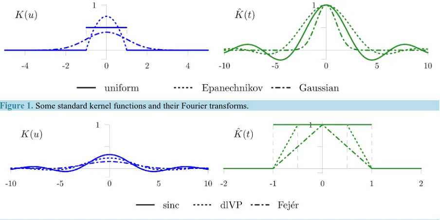
Some classical examples of kernels together with their Fourier transforms (see formula (6)) are listed in Table 1 and presented graphically in Figure 1. These kernel functions are the most commonly applied in practice, most likely due to their additional nonnegative property as their corresponding estimators result in density functions. The group of kernels listed in Table 2 and presented in Figure 2, along with their Fourier transforms, are well known in statistical theory and generally more asymptotically efficient than the standard kernels in
Table 1 since they were shown to achieve better rates of convergence in the works of [2][9]. These kernel functions alternate between positive and negative values, except for the Fejér kernel. For these kernels, the
positive part estimator
( )
: max 0,{
( )
}
n n
f+ x = f x
can be used to maintain the positivity of a density estimator. Throughout our analysis, we shall be using the positive part of all the kernel density estimators under study.
[image:5.595.87.539.480.706.2]The most popular approach for judging the quality of an estimator in the literature and in practice is the Mean
Figure 1. Some standard kernel functions and their Fourier transforms.
Table 1. Some standard kernel functions and their Fourier transforms.
Kernel K u( ) ˆ( ) eitu ( )d
K t =
∫
K u u
uniform 1
(
1)
2 u≤
( )
sin
if 0, 1 if 0
t t t t ≠ =
Epanechnikov 3
(
2) (
)
1 1
4 −u u≤
( ) ( )
(
)
3
3
sin cos if 0,
1 if 0
t t t t
t t − ≠ =
Gaussian 1 22
e 2π
u
− 22
e−t
Table 2. Some efficient kernel functions and their Fourier transforms.
Kernel K u( ) ˆ( ) eitu ( )d
K t =
∫
K u u sinc ( ) sin if 0, π 1 if 0 π u u u u ≠ =
(
t≤1)
de la Vallée Poussin
( ) ( )
(
)
2
2 cos 2 cos
if 0, π 3 if 0 4π u u u u u − ≠ =
(
)
1 12 1 1
2 2
t t t
≤ + − < <
Fejér ( ) 2 2 2sin 2 if 0, π 1 if 0 2π u u u u ≠ =
(
1−t) (
t≤1)
Integrated Squared Error (MISE). Observe that the 2-risk, as in (3), with
( )
2l x =x is simply the MISE defined as
(
)
(
2)
(
( )
( )
)
22
MISE fn,f :=l fn− f =
∫
fn x − f x dx. (5)By the Fubini theorem, the right-hand side (RHS) of (5) can be further expanded to represent the variance- bias decomposition of the density estimator:
(
)
(
( )
( )
)
(
( )
( )
)
( )
( )
2
2 2
2 2
MISE , d d
: d d .
n n n n
n n
f f f x f x x f x f x x
x x b x x
σ = − + − = +
∫
∫
∫
∫
Notice also that the MISE of the positive part estimator fn
+
satisfies
(
)
(
)
MISE fn ,f MISE fn,f .
+ ≤
3.1. Fourier Analysis of Kernel Density Estimators
[image:6.595.90.536.282.489.2]simpler form than those of the standard kernels. This simplifies the analysis of density estimators under certain settings when using efficient kernel functions. We begin by providing a few basic definitions and properties related to the Fourier transform (see, for example, Chapter 9 of [10]).
The Fourier transform gˆ of a function g∈ 1
( )
is defined by( )
( )
ˆ : eitx d , ,
g t =
∫
g x x t∈ (6)where i= −1. The Plancherel theorem allows us to extend the definition of the Fourier transform to functions in 2
( )
. Moreover, for any g∈ 2( )
, the Parseval formula holds true:( )
2 1( )
2ˆ
d d .
2π
g x x= g t t
∫
∫
(7)Using also the notation g
( )
⋅( )
t for the Fourier transform of g∈ 2( )
at t, for any h>0 and x∈
( )
( )
(
)
( )
( )
1
ˆ , eitxˆ , .
g t g ht g x t g t t
h h
⋅
= − ⋅ = − ∈
(8)
The Fourier transform of a density is known to be the characteristic function defined by
( )
t : eitxf x( )
dx e ditx F x( )
, t .ϕ =
∫
=∫
∈
The corresponding empirical characteristic function is
( )
(
1)
( )
1
1
: ; , , e d e , ,
n iX t itx j
n n n n
j
t t X X F x t
n ϕ ϕ = = =
∫
=∑
∈ where F xn
( )
n1 nj1(
Xj x)
− =
=
∑
≤ , and has the following properties that follow one after the other:( )
( )
( )
( )
( )
( )
(
( )
)
2 2 2 2 , 1 1 1 , 1 1 , n n n t t t t n nt t t
n
ϕ ϕ
ϕ ϕ
ϕ ϕ ϕ
= = − + − = − (9)
for all t∈. Given the properties in (8) and the symmetry of K, the Fourier transform fˆn of the density
estimator fn can be expressed as follows:
( )
(
)
( )
( )
( ) ( )
1 1
1 1
ˆ e j ˆ ˆ .
n n
itX
n h j n
j j
f t K X t K ht t K ht
n = n = ϕ
=
∑
− ⋅ =∑
= (10)In 2-theory, the MISE can also be expressed using the Fourier analysis of kernel density estimators. Indeed
according to (7), assuming that f and K are both in 2
( )
and that K is symmetric, the MISE satisfies(
)
(
( )
( )
)
2 1 ˆ( )
ˆ( )
2MISE , d d .
2π
n n n
f f = f x − f x x= f t − f t t
∫
∫
Continuing from (10) and relations (9), the MISE of the kernel estimator fn of density f takes the form (see
Theorem 1.4 of [11])
(
)
( )
( )
( )
( )
( )
(
)
2 2 2
2 2
1 ˆ 1 ˆ
MISE , 1 d d
2π
1 ˆ
d : , , , 2π
n
n
f f K ht t t K ht t
n
t K ht t J K h
n ϕ ϕ ϕ = − + − =
∫
∫
∫
(11)where f K, ∈ 2
( )
, n≥1, and h>0.optimal kernels. Indeed, most of the general properties of a kernel in (4), such as K integrating to one or being an integrable function, do not need to be true. Also, the expression for Jn
(
K h, ,ϕ)
in (11) makes it possible to easily determine inadmissible kernel functions in 2( )
for any fixed n. Recall that a kernel is calledinadmissible if there exist other kernels in 2
( )
that can improve Jn(
K h, ,ϕ)
for all characteristic func-tions in 2
( )
. A simple method for detecting inadmissible kernels was presented by Cline [13]: if( )
[ ]
(
ˆ)
Leb t K t: ∉ 0,1 >0, (12)
where Leb(A) denotes the Lebesgue measure of a set A, then K is inadmissible. As seen from Figure 1, the Epanechnikov and uniform kernel functions are inadmissible since the set
{
t K t: ˆ( )
∉[ ]
0,1}
has a positive Lebesgue measure. This is another argument as to why the efficient kernels listed in Table 2 as well as the family of Fejér-type kernels in (20) are preferred.3.2. Bandwidth Selection Based on Unbiased Risk Estimation and Fourier Analysis Techniques
Selecting an appropriate bandwidth h=hn, that is dependent on the sample size, is very important as it
determines the smoothness of the kernel density estimator. A small bandwidth produces a peaky-like estimator indicative of high variability caused by under-smoothing. On the other hand, a large bandwidth increases the bias of the estimator and the important features of the distribution may be lost due to over-smoothing. The aim is to choose a bandwidth that minimizes the bias and the variance of an estimator to avoid over- or under- smoothing, a dilemma known as the bias-variance tradeoff.
In theory, an optimal bandwidth can be obtained by minimizing the MISE with respect to h:
( )
0
arg min MISE .
opt h
h h
>
= (13)
In practice, the RHS of (13) cannot be computed as the MISE depends on the unknown density f. Instead, an approximately unbiased estimator of the MISE
( )
h computed from the random sample X1,,Xn is mini-mized. The idea is to consider the expansion of the MISE in (5) in the following way
( )
2( )
( ) ( )
2( )
( )
2( )
MISE h =
∫
fn x dx−2∫
fn x f x dx+∫
f x dx=: n h +∫
f x d .x
As we are only concerned with minimizing the MISE with respect to h, the term
∫
f2( )
x dx may be disregarded. The estimator( )
2( )
( )
, 1
2
CV : d ,
n
n n j j j
h f x x f X n = −
=
∫
−∑
where( ) ( )
, 1 : 1 k n j k j X xf x K
n h h
− ≠ − = −
∑
is the leave-one-out estimator of f x
( )
, is an unbiased estimator of n( )
h . The function CV( )
⋅ is called theunbiased cross-validation criterion, which can by further expanded to (see [14], p. 55)
( )
(
)
(
)
(
)( )
(
)
(
)
2
1 1 1
2 1 1 1 1 1 2 CV 1 1 2 0 4 , 1
n n n n
j k j k
j k j k j
k n
j k j k j
k n
j k j k j
X X X X
h K K K
h n n h h
n h
X X
K K K K
nh n h h
X X K
nh n h
= = = ≠ = = + = = + − − = ∗ − − − = ∗ + ∗ − − −
∑∑
∑∑
∑ ∑
∑ ∑
(14)minimums for the values of hopt. In practice, it is expected that, for a random sample X1,,Xn, the minimizer
of CV
( )
h is close to the minimizer of CV( )
h . The cross-validation bandwidth is therefore given by(
)
CV 1
0
: arg min CV ; , , n ,
h
h h X X
>
= (15)
yielding
( )
,CV 1 CV CV 1 : n j n j X xf x K
nh = h −
=
∑
as the kernel estimator of f x
( )
specified by hCV. Selecting bandwidths using the unbiased cross-validationcriterion of the form above was first introduced by Rudemo in [15].
Cross-validation is perhaps the most common approach based on unbiased risk estimation for selecting h; however, many authors have noted that is has a slow rate of convergence towards hopt in (13) (see [16],
Theorem 4.1). Another parallel method is to minimize an unbiased estimator of the MISE based on the Fourier analysis of kernel density estimators over h. The latter method for selecting a bandwidth is due to Golubev [17]
and is shown to provide more reliable results in our simulation study in Section 5 than the cross-validation approach. For this reason, we shall use this method to select our bandwidth in the VaR computation model proposed in Section 6.
The MISE of interest is given in (11) and denoted by Jn
(
K h, ,ϕ)
. Golubev [17] found an approximately unbiased estimator of Jn(
K h, ,ϕ)
given by( )
ˆ( )
ˆ2( )
1( )
2 2 ˆ( )
: 2 1 d d ,
n n
J h K ht K ht t t K ht t
n ϕ n
= − + − +
∫
∫
(16)
where h>0. Indeed, from relations (9) we get that, up to scaling and shifting, Jn
( )
h is an unbiased estimatorof Jn
(
K h, ,ϕ)
:( )
1(
)
2( )
2π 1 , , d .
n n
J h J K h f x x
n ϕ
= − −
∫
Hence, minimizing Jn
( )
h is equivalent to minimizing Jn(
K h, ,ϕ)
over h. In practice, an approximateminimizer of Jn
(
K h, ,ϕ)
is obtained by using the random sample X1,,Xn to compute Jn( )
h and thenminimized with respect to h:
(
)
F 1
0
: arg min n ; , , n .
h
h J h X X
>
= (17)
The corresponding kernel density estimator with the bandwidth hF is then
( )
,F 1 F F 1 : . n j n j X xf x K
nh = h −
=
∑
Under appropriate conditions, hF and hCV are asymptotically optimal as they are asymptotically equivalent
to hopt in (13). In other words, the MISE of the kernel density estimators fn,F and fn,CV is asymptotically
equivalent to that of the estimator with the optimal bandwidth hopt (see Section 1.4 of [11]).
4. Density Estimators with Fejér-Type Kernel Functions
Suppose that X X1, 2, is a sequence of iid random variables on with a common density function f from
some functional class . Consider the functional class γ =
(
γ,L)
of functions f in 2( )
such that eachf∈γ admits an analytic continuation to the strip Sγ =
{
x+iy: y ≤γ}
with γ >0 such that f x(
+iy)
isanalytic on the interior of Sγ, bounded on Sγ, and for some L>0
(
)
2 .f ⋅ ±iγ ≤L
We have for any f∈γ
( ) ( )
22
1 ˆ
cosh d .
The functional class γ is well known in approximation theory (see, for example, [18], Section 94) and widely
used in nonparametric estimation (see [2]-[5] [19] [20]). For certain values of γ , the class γ contains probability densities such as the normal, Student’s t, and Cauchy as well as their analytic transformations and mixtures. The inequality in (18) is used in [12] to determine how large the values of γ can be chosen so that these probability densities belong to γ. The normal, Student’s t with odd degrees of freedom ν, and stand-
ard Cauchy density function are in the analytical class γ with γ >0, 0< <γ ν , and 0< <γ 1, respec-
tively. For other examples of functions belonging to γ we refer to Section 2.3 of [21].
The kernel-type estimator of f ∈γ considered in this work has the form
(
)
(
1)
1
1
; : ; , , , ; , ,
n j
n n n n n n n
j
n n
X x
f x f x X X K x
nh h
θ θ θ
= − = = ∈
∑
(19)
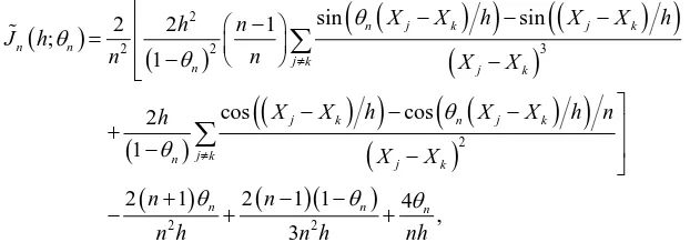
where Kn is the Fejér-type kernel given by
(
)
( )
( )
(
)
2cos cos if 0, π 1 ; : 1 if 0, 2π n n n n n u u u u K u u θ θ θ θ − ≠ − = + = (20) with 1 log
, 1 , .
2 n n n n h M M M θ θ γ
= = − = (21)
It is easy to see that the Fejér-type kernel as in (20) satisfies the properties in (4). The parameters in (21) are chosen to have
0 and as ,
n n
h → nh → ∞ n→ ∞
ensuring the consistency of fn
(
x;θn)
in (19) as an estimator of f x( )
. Moreover, the kernel-type density estimator as in (20) with the bandwidth hn satisfying (21) is known to have very small p-risk, 1≤ < ∞p(see Theorem 1 of [2]). For some choices of 0≤θn<1, Table 3 shows how the Fejér-type kernel coincides with the well-known efficient kernels listed in Table 2. The sinc kernel is the limiting case of the Fejér-type kernel when θn→1; in other words, when n approaches infinity. Additionally, choosing θn=1 2 and θn=0 leads to the de le Vallée Poussin and Fejér kernels, respectively.
The Fourier transform of the Fejér-type kernel is given by (see [18], p. 202)
(
)
(
)
(
)
1(
)
ˆ ; e ; d 1 .
1
itu
n n n n n n
n
t
K t θ K uθ u t θ θ t
θ − = = ≤ + ≤ ≤ −
∫
The Fejér-type kernel Kn and its Fourier transform Kˆn are presented graphically in Figure 3. Observe the simple form of Kˆn, which makes it very useful in studying analytically the properties of the estimator in (19). Also, Kˆn is nonnegative and bounded by one making the Fejér-type kernel admissible according to the Cline criterion as in (12).
[image:10.595.86.539.636.719.2]To apply the data-driven bandwidths given in (15) and (17), the unbiased estimators as in (14) and (16), denoted by CV
( )
h and Jn( )
h , need to be evaluated for the Fejér-type kernel. The unbiased cross-validation criterion CV( )
h includes the convolution of the kernel with itself. The self-convolution of the Fejér-type kernel is given by (see p. 44 of [12] for details)Table 3. Cases of the Fejér-type kernel.
Kernel θn
sinc 1
de la Vallée Poussin 1/2
Figure 3. The Fejér-type kernel function and its Fourier transform.
(
)(
)
( )
(
)
2(
( )
(
)
2 3( )
)
2 sin sin 2 cos
if 0,
π 1 π 1
; 1 2 if 0, 3π n n n n
n n n
n
u u
u
u
u u
K K u
u θ θ θ θ θ θ − + ≠ − − ∗ = + =
where 0≤θn<1 for n>1. It can be shown (see [12], p. 48) that the unbiased risk estimator based on the Fourier analysis of a density estimator with the Fejér-type kernel is given by:
(
)
(
)
(
)
(
)
(
(
)
)
(
)
(
)
(
)
(
)
(
(
)
)
(
)
(
)
(
)(
)
22 2 3
2
2 2
sin sin
2 2 1
;
1
cos cos
2 1
2 1 1
2 1 4
, 3
n j k j k
n n
j k
n j k
j k n j k
j k
n j k
n
n n
X X h X X h
h n
J h
n
n X X
X X h X X h n
h
X X
n n
nh
n h n h
θ θ θ θ θ θ θ θ ≠ ≠ − − − − = − − − − − + − − − − + − + +
∑
∑
for n>1, h>0, 0≤θn<1, and Xj ≠Xk, 1≤ ≠ ≤j k n. Note that in the case of sampling from a continuous
distribution P X
(
j ≠Xk)
=1,1≤ ≠ ≤j k n.In the following section, we demonstrate numerically that the positive part of the kernel-type estimator in (19) with the Fejér-type kernel in (20) works well with respect to the 2-risk for both theoretical and empirical
bandwidth selectors.
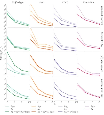
5. Simulation Study: Comparison of Kernel Density Estimators
A simulation study is carried out to assess the quality of the positive part of the density estimator in (19) with the Fejér-type kernel in (20) using the MISE criterion. The finite-sample performance of (19) is compared to other density estimators that use the sinc, de la Vallée Poussin, and Gaussian kernels. These kernel functions were chosen since the sinc and de la Vallée Poussin are efficient kernels that are specific cases of the Fejér-type, while the Gaussian kernel is the most commonly used in practice. Three bandwidth selectors are applied to the kernel density estimators in hand. The bandwidth selection methods include the empirical approaches from cross-validation and Fourier analysis and the theoretical smoothing parameter hn =
(
2γθn)
logn, which is used for density estimators with efficient kernels. From here on, we shall refer to the bandwidth hF in (17) as theFourier bandwidth.
We generated 200 random samples, of a wide range of sample sizes, from the following four distributions: standard normal N
( )
0,1 , Student’s t15 with 15 degrees of freedom, chi-square2 4
χ with 4 degrees of freedom, and normal mixture 0.4N
( )
0,1 +0.6N(
1, 0.42)
. These distributions were chosen as their density func- tions cover different shapes and characteristics such as: symmetry, skewness, unimodality, and bimodality. The chi-square is the only one out of these distributions whose density function f is not in the functional class γconduct the experiments refer to Section 4.1 of [12].
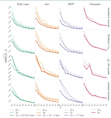
Let us first assess the bandwidth selection methods under consideration. Figure 4 and Figure 5 capture the performance of each bandwidth selection method for each kernel density estimate under study by plotting the MISE estimates against samples of size 25 to 100 and 200 to 1000, respectively. The following can be observed from the figures. For a good choice of γ , the estimates of f∈γ with efficient kernel functions and theo-
[image:12.595.97.537.182.666.2]retical bandwidths complement the results of Theorem 1 in [2] and Theorem 2 in [6] by outperforming the estimates with empirical bandwidths. The theoretical estimates do not perform as well, though, when estimating
Figure 4. MISE estimates for the cross-validation, Fourier, and theoretical bandwidth selectors with Fejér-type, sinc, dlVP, and Gaussian kernels that estimate the standard normal, Student’s t15, chi-square 2
4
χ , and normal mixture, for small sample sizes. The MISE estimates are averaged over 200 replications. The symbol * denotes the manually-selected γ that provided
Figure 5. MISE estimates for the cross-validation, Fourier, and theoretical bandwidth selectors with Fejér-type, sinc, dlVP, and Gaussian kernels that estimate the standard normal, Student’s t15, chi-square 2
4
χ , and normal mixture, for large sample sizes. The MISE estimates are averaged over 200 replications. The symbol ∗ denotes the manually-selected γ that pro-
vided good results.
the chi-square density, which is not in γ , particularly for smaller sample sizes. Generally speaking, it can also
be seen that, when estimating the unimodal densities, the bandwidth based on the Fourier analysis techniques is better than, or equal to, the cross-validation bandwidth. The difference in estimation error is especially notice- able for smaller sample sizes.
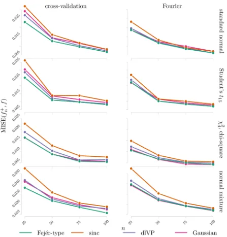
Now, we assess the quality of the Fejér-type kernel estimator when using empirical bandwidths. Figure 6 and
Figure 6. MISE estimates for the Fejér-type, sinc, dlVP, and Gaussian kernels with cross-validation and Fourier bandwidth selectors that estimate a standard normal, Student’s t15, chi-square
2 4
χ , and normal mixture, for small sample sizes. The
MISE estimates are averaged over 200 replications.
estimation of the unimodal densities with data-dependent bandwidth methods, the Fejér-type kernel slightly improves the other fixed efficient kernels and performs much better than the common Gaussian kernel for larger sample sizes. Also, we observe that, when estimating the bimodal density, the Fejér-type kernel performs much better than all of the competing kernels, especially for large sample sizes.
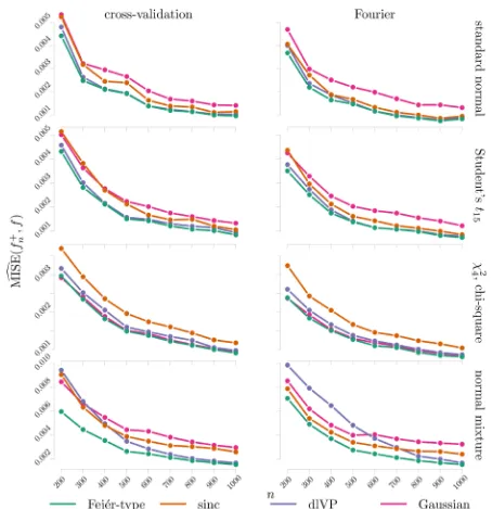
Figure 7. MISE estimates for the Fejér-type, sinc, dlVP, and Gaussian kernels with cross-validation and Fourier bandwidth selectors that estimate a standard normal, Student’s t15, chi-square 2
4
χ , and normal mixture, for large sample sizes. The
MISE estimates are averaged over 200 replications.
MISE, with competing kernel estimators, especially when estimating normal mixtures. The simulation results attest that, for a good choice of γ, the estimator with the Fejér-type kernel performs very well when using both empirical and theoretical bandwidths to estimate densities in γ and therefore is reliable in application.
6. VaR Model with Fejér-Type Kernel Functions
Suppose that X1,,Xn is a random sample of iid portfolio returns with an absolutely continuous cdf F on ,
and let
( )1 ( )2 ( )n
denote the corresponding order statistics. Recall that VaR models are concerned with evaluating a quantile function Q p
( )
, 0< <p 1, defined as( )
1( )
{
( )
}
: inf :
Q p =F− p = x F x ≥p
for a general cdf F x
( )
that is continuous from the right. We are interested in estimating a quantile function using the Fejér-type kernel function in (20).Let F xn
( )
be the empirical distribution function given by( )
(
)
1 1 : , . n n j jF x X x x
n =
=
∑
≤ ∈By Kolmogorov’s strong law of large numbers, the empirical distribution function is a strongly consistent estimator of the true distribution for any x∈, that is,
( )
. .( )
, .
a s n n
F x →∞→F x x∈
Moreover, by the Glivenko-Cantelli theorem,
( )
( )
. .sup n na s 0.
x
F x F x →∞ ∈ − →
A common definition for the empirical quantile function is
( )
: 1( )
( )n n j
Q p =F− p =X
for
(
j−1)
n< ≤p j n, j=1,,n. In 1979, Parzen (see [22], p. 113) introduced the kernel quantile estimator( )
(
) ( )
(
)
( )
( )(
)
( )1 1 1
0 0 1
1
d d : d ,
n j n
n h n h n j n h j
j
KQ p K t p Q t t K t p F− t t − K t p t X =
= − = − = −
∑
∫
∫
∫
(22)where 0< <p 1 and for a suitable kernel function K, Kh
( )
x h K h x1( )
1− −
= . Naturally, KQn
( )
p puts mostweight on the order statistic X( )j , for which j n is close to p. Sheather and Marron [23] showed that the following approximation to KQn
( )
p as in (22) can be used in practice:
( )
1 ( )1 1 2 . 1 2 n h j j n n h j j
K p X
n KQ p j K p n = = − − = − −
∑
∑
Therefore, for a probability level p∈
( )
0,1 , we suggest that the VaR estimator can be computed as
( )
F ( )F 1 3, 1 1 2 ; VaR , 1 2 ; n
h n j
j n n h n j j
K p X
n p j K p n θ θ = = − − = − −
∑
∑
(23)where KhF is the scaled Fejér-type kernel function based on (20) and hF is the bandwidth in (17), referred to
as the Fourier bandwidth. The bandwidth obtained from Fourier analysis methods was chosen as it provided good results in the simulation studies in Section 5.
7. Application to Value at Risk
We assess the proposed nonparametric VaR computation method given by formula (23) and compare it to the common normal and historical simulation approaches as in (1) and (2). Each VaR computation method is evaluated by means of a statistical back-test procedure based on a likelihood ratio test.
7.1. Evaluation of VaR Computation Methods
VaR of the portfolio should fall within a specified confidence level; otherwise, the model is rejected as it is not considered adequate for predicting the VaR of a portfolio. A back-test of this form was first used by Kupiec in 1995 (see [1], Chapter 6).
Let X X1, 2, be a sequence of iid random portfolio returns with a common density f on X X1, 2,. In our
analysis, we consider two different samples; an estimation sample of size n for computing the VaR and an evaluation sample of size m for comparing the estimated VaR returns with the actual returns. Let Y1,,Ym be
iid random variables that indicate whether or not the realized return is worse than the predicted VaR measure, that is,
( )
( )
1 1 11 if VaR ,
, 0, , 1,
0 if VaR ,
t t t
t t
X p
Y t m
X p + + + ≤
= > = −
where P X
(
t+1≤VaRt( )
p)
=p. Then, 1 mi i
N =
∑
=Y is the number of estimated VaR violations of a portfolio out of an evaluation sample of m observations and follows the binomial distribution Bin m p(
,)
with pro- bability mass function (pmf)(
;)
m y(
1)
m y,P N y p p p y
−
= = −
for y=0,1,,m. Suppose the probability level for the VaR is chosen to be p0. The ratio N m represents
the failure rate of the VaR model, which under the null hypothesis specified below converges to p0. The
relevant null and alternative hypotheses for determining the fit of the VaR model are given by
0: 0 vs. 1: 0.
H p= p H p≠ p
A likelihood ratio test is carried out to determine whether or not to reject the null hypothesis that the model is adequate. The likelihood function for p given the observed values y1,,ym of Y1,,Ym is
(
)
(
)
(
)
1(
)
1
1 1
| , , ; i i 1 ,
m m
y m y
y y
m i i
i i
L p y y P Y y p p i p − p p −
= =
=
∏
= =∏
− = − (24)
where y=
∑
mi=1yi. Following from (24), the appropriate likelihood ratio test statistic is given by( )
(
)
(
)
(
)
(
) (
)
0 0
0 1
0 0 1
1
1 ( | , , )
| , , ,
| , , / 1 /
m y y
m
m y m y
m
p p
L p y y
p p y y
L y m y y y m y m
−
−
−
Λ = Λ = =
−
where y1,,ym are the observed values of Y1,,Ym, and 1 m
i i
y=
∑
=y is the outcome of N=∑
mi=1Yi. Undermild regularity conditions, the asymptotic distribution of the log-likelihood ratio statistic −2 log
(
Λ( )
p0)
=(
)
(
0 1)
2 log p |Y, ,Ym
− Λ under H0 is
(
)
2 1 1χ −α as m approaches infinity (see [24], Chapter 13, Theorem 6). Thus, if
( )
(
)
2(
)
0 1
2 log p χ 1 α ,
− Λ > −
we would reject H0 that the failure rate of the model is reasonable at level α. Typically, the α is set at 0.05.
Therefore, we reject the null hypothesis if
( )
(
)
2(
)
0 1
2 log p χ 0.95 3.841459.
− Λ > ≈
In this study, we evaluate the test statistic −2 log
(
Λ( )
p0)
for the 0.05, 0.025, 0.01, and 0.005 probabilitylevels and evaluation samples of size 250, 500, 750, and 1000. The acceptable number of failures in a VaR model are displayed in Table 4. The VaR model can be rejected when the number of failures is both high and low. If there are too many exceptions, the model underestimates the VaR. On the other hand, if there are too few exceptions, then the model is too conservative and can harm profit opportunities.
7.2. Comparative Study of VaR Computation Methods
0.025, 0.01, and 0.005 are considered. Each VaR model is estimated using samples of 252, 504, and 1000 trading days. A back-test is then performed to evaluate the adequacy of each VaR model under consideration over an evaluation sample of 1000 trading days.
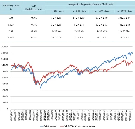
We have two imaginary investment portfolios each consisting of a single well-known stock index, the Dow Jones Industrial Average (DJIA) and the S&P/TSX Composite Index. These indices were chosen to be in our fictitious portfolios as they have abundant publicly available historical data. Here, they are used as repre- sentative stocks since, in reality, an index cannot be invested directly being that it is a mathematical construct. The raw values of the daily DJIA and S&P/TSX Composite indices are displayed in Figure 8 from June 28, 2007 to March 11, 2015. The effect of the 2008 financial crisis is indicated by both indices, where the DJIA can be seen to have a large decrease in points with a low level of approximately 6500 in the early months of 2009. This is followed by an increase in the level of both indices in the recent years, particularly for the DJIA.
The index values are used to evaluate the daily logarithmic returns as follows. If Pt+1 and Pt are the index
[image:18.595.88.535.277.706.2]values at time t+1 and t, respectively, then the return Xt+1 at time t+1 is given by
Table 4. 95% nonrejection confidence regions for the likelihood ratio test under different VaR confidence levels and
evaluation sample sizes.
Probability Level
0
p
VaR Confidence Level
Nonrejection Region for Number of Failures N
250
m= days m=500 days m=750 days m=1000 days 0.05 95.0% 7≤N≤19 17≤N≤35 27≤N≤49 38≤N≤64 0.025 97.5% 3≤N≤11 7≤N≤19 12≤N≤17 16≤N≤35 0.01 99.0% 1≤N≤6 2≤N≤9 3≤N≤13 5≤N≤16 0.005 99.5% 0≤N≤5 1≤N≤6 1≤N≤8 2≤N≤9
(
)
1 log 1 .
t t t
X+ = P+ P
The autocorrelation of the daily log returns are plotted in Figure 9 for each index. We can observe that there are no significant autocorrelations as almost all of them fall within the 95% confidence limits. A few lags slightly outside of the limits do not necessarily indicate non-randomness as this can be expected due to random fluctuations. In addition, there is absence of a pattern. Therefore, both portfolios may be considered random, and thus all the VaR computation methods in hand may be applied.
The daily log returns and VaR estimates for every model under consideration are displayed in Figure 10 and
Figure 11 for each stock index over a time period of one thousand trading days. Each row of plots corresponds to the VaR confidence level, while each column provides the results of the estimation sample used. Table 5
[image:19.595.89.535.286.719.2]displays the back-test results of all the VaR models in question for each stock market index. The outcome of each test, that is whether or not to reject the model given the observed number of VaR violations, is reported for every VaR model. These outcomes are determined by the 95% nonrejection regions indicated in Table 4 when the evaluation sample size is 1000 days.
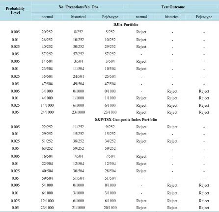
Table 5. Back-test results of all the VaR models under consideration applied to each stock index over an evaluation sample
of 1000 days and 95% confidence regions.
Probability Level
No. Exceptions/No. Obs. Test Outcome
normal historical Fejér-type normal historical Fejér-type
DJIA Portfolio
0.005 20/252 8/252 5/252 Reject - -
0.01 26/252 10/252 10/252 Reject - -
0.025 40/252 30/252 29/252 Reject - -
0.05 57/252 57/252 57/252 - - -
0.005 14/504 3/504 3/504 Reject - -
0.01 23/504 11/504 10/504 Reject - -
0.025 35/504 24/504 25/504 - - -
0.05 47/504 49/504 47/504 - - -
0.005 3/1000 0/1000 0/1000 - Reject Reject 0.01 4/1000 1/1000 1/1000 Reject Reject Reject 0.025 14/1000 6/1000 6/1000 Reject Reject Reject 0.05 24/1000 23/1000 23/1000 Reject Reject Reject
S&P/TSX Composite Index Portfolio
0.005 22/252 11/252 9/252 Reject Reject -
0.01 29/252 15/252 15/252 Reject - -
0.025 51/252 38/252 34/252 Reject Reject -
0.05 63/252 59/252 59/252 - - -
0.005 16/504 7/504 7/504 Reject - -
0.01 22/504 12/504 12/504 Reject - -
0.025 40/504 30/504 28/504 Reject - -
0.05 59/504 51/504 51/504 - - -
0.005 5/1000 0/1000 0/1000 - Reject Reject
0.01 6/1000 3/1000 3/1000 - Reject Reject
Figure 9. Autocorrelation plots of the daily logarithmic returns for each stock market index.
The following can be observed from the aforementioned figures and tables. Overall, the empirical results of both stock indices are fairly similar. The back-test results in Table 5 show that the normal model has the poorest performance as it is not considered adequate in most cases. The observed number of VaR violations is quite high for smaller probability levels, meaning that the mass in the tails of the distribution is underestimated. The only case when the normal model is not consistently rejected is when the probability level is 0.05 for estimation samples of 252 and 504 observations. The historical simulation method generally performs well and shares similar results with the newly proposed VaR estimation method. It is, however, rejected for probability levels 0.005 and 0.025 when the number of observations is 252 in the S&P/TSX Composite Index portfolio. Finally, the VaR model of interest based on the Fejér-type kernel quantile estimation is the most reliable as it has the least number of rejections for all the tests considered.
Overall, it can be seen that none of the models perform well when the estimation sample is large, except for sometimes the normal method when probability levels are small. This is expected as financial data from four years ago may no longer be relevant to the current market situation. Moreover, the performance of all the VaR computation methods is similar at the 95% confidence level.
For an illustration of the density of portfolio returns on a specific day see Figure 12 and Figure 13. The Fejér-type kernel density estimates with Fourier bandwidths are represented by the green curves while the normal densities have the red curves. The images are consistent with the assertion that the stock returns are heavy tailed. It can be clearly seen that the density estimates with Fejér-type kernels can account for heavy tails of the return distributions better than the normal densities.
In summary, the proposed method for computing the VaR based on density estimation with Fejér-type kernel functions and Fourier analysis bandwidth selectors provides more reliable results than the commonly used VaR computation methods. Density estimates with Fejér-type kernel functions can account for the heavy tails of the return distributions, unlike the normal density. The normal method for computing the VaR tends to underesti- mate the risk, especially for higher confidence levels. For the nonparametric models, one has to be careful in choosing a relevant estimation period; otherwise, they tend to overestimate the risk for large estimation samples.
8. Conclusion
The paper introduces a nonparametric method of VaR computation on portfolio returns. The approach relies on the kernel quantile estimator introduced by Parzen [22]. The kernel functions employed are Fejér-type kernel functions. We use these functions because they are known to produce asymptotically efficient kernel density estimators with respect to the 2-risk. A simulation study in support of this theoretical result is first conducted,
Figure 10. Daily log returns and VaR estimates of the DJIA at 95%, 97.5%, 99%, and 99.5% confidence levels under 252,
504, and 1000 observations over 1000 trading days for the VaR computation methods in consideration.
Figure 11. Daily log returns and VaR estimates of the S&P/TSX Composite Index at 95%, 97.5%, 99%, and 99.5% confidence levels under 252, 504, and 1000 observations over 1000 trading days for the VaR computation methods in
consideration.
numerical results. The resulting estimator is compared numerically with the two standard VaR estimators,
1,
( )
Figure 12. Normal, empirical, and positive part Fejér-type kernel densities of the DJIA daily returns based on 252, 504, and 1000 observations for the days 29/06/2011, 25/06/2013, and 30/09/2014. The 97.5% VaR of each model is illustrated along
with the actual daily return.
Figure 13. Normal, empirical, and positive part Fejér-type kernel densities of the S&P/TSX Composite daily returns based on 252, 504, and 1000 observations for the days 29/06/2011, 25/06/2013, and 30/09/2014. The 97.5% VaR of each model is
illustrated along with the actual daily return.