Performance Enhancement for Tsunami Wave
Simulation using Hexagonal Cellular Automata
E.Syed Mohamed¹
Computer Science and Engineering Department, B.S.Abdur Rahman University,Vandalur
Chennai 600 048, INDIA
S.Rajasekaran²
Mathematics Department, B.S.Abdur Rahman University, Vandalur
Chennai 600 048, INDIA
ABSTRACT
Tsunamis are considered the most devastating natural hazard on costal environments ever known. Early tsunami wave detection, both quick and appropriate intervention is of vital importance for minimization tsunami damage. Simulation of tsunami wave spread remains a daunting task due to factors such as complex wave behavior, dynamical wave condition and large spatial data that needs to be modelled. In this paper tsunami wave models have been widely studied using cellular automata(CA) that has special features for simulating complex phenomena .The influential factors for tsunami wave are divided into two categories and our models are applied to eight basic cases depending on weather, topography and wave conditions for different rates of spread. The algorithm is efficient and easily implemented, allowing less computational time and cost. Experimental results of this model prove its value in tsunami wave spread as real time.
Key words
Tsunami wave, Simulation, Homogeneous,
Non-homogeneous, Cellular automata, Discrete time step, Primary wave front, Secondary wave front
1. INTRODUCTION
A significant deformation of an ocean floor caused by an underwater earthquake, landslide or volcanic eruption produces a tsunami wave on the ocean surface. Once the tsunami is generated, it propagates into more and more shallow ocean, and its propagation is influenced by the depth of the ocean. Since the energy of the tsunami is dissipated by the death of the ocean [1]. It is found that the propagation of the tsunamis depends on the relative magnitude of the given speed of the running speed of the running ocean and the wave speed of Shallow Ocean. Nowadays, assessing hazard conditions related to complex natural phenomena increasingly takes advantage of computer-assisted analyses and simulations. To study the tsunami wave, tsunamis are divided in to a matrix of identical square cells, with side length L, and it is represented by a CA.
The remainder of the section is organized as follows: Section2 describes the related works available in the literature. In section3, the assumptions are used in cellular automata model. Section 4 describes multi models of cellular automata for tsunami wave spread. In section 5 the implementation of homogeneous hexagonal cellular automata models are proposed and several tests for the new models are checked and their simulation are shown. In Section 6, the implementation of non-homogeneous Hexagonal cellular
automata model is proposed and several tests for the new models are checked and their simulations are shown. In Section 7, comparison with two-dimensional square cellular automata graph results shown and finally, the conclusions are presented in the paper
2.
RELATED
WORKS
IN
THE
LITERATURE
In the open ocean a tsunami is less than a few feet high at the surface, but its wave height increases rapidly in shallow water. But, as the tsunami reaches shallower coastal waters, wave height can increase rapidly [2] [3]
A trans-oceanic tsunami is one that propagates throughout the ocean in which it is generated and could cause loss of life and damage even far away from the epicenter area. Second, an ocean-wide tsunami is one which propagates throughout the ocean in which it is generated, but the loss of life and damage are mostly confined to the epicenter area [4]
For a tsunami generated by pure thrust faulting, only the primary wave fronts would be evident: one moving toward the deep ocean and one moving toward the local shoreline In addition, there is a secondary wave front propagating to the northeast that is a continuation of the shoreward primary wave front. Both of the secondary wave fronts initially travel parallel to shoreline, but their paths of travel curve (refract) toward shore.
Physics tells us that when the energy in a system remains constant, but velocity decreases, the mass in the system must increase. A slower moving tsunami is a physically higher tsunami. The waves scrunch together like the ribs of an accordion and heave upward. [5]
In this work, a new cellular automaton model based on the transfer of fractional traversed area for tsunami propagation in real time simulation and visualization is proposed [6].
3. ASSUMPTIONS USED IN CELLULAR
AUTOMATA MODEL
A cellular automaton is an array of 'cells' that interact with their neighbours. These arrays can take on any number of dimensions, starting from a one dimensional string of cells. Each cell has its own state that can be a variable, property or other information.
At the beginning of the simulation, cell states are initialized by means of input matrices. Moore’s model parameters have also to be assigned in this phase, by taking into consideration their physical/empirical meaning. By simultaneously applying the transition function to all the cells, at discrete steps, states are changed and the evolution of the phenomenon can be simulated
[image:2.595.328.522.183.271.2]A tsunami wave model represented as a two-dimensional cell-space composed of cells of dimensions ℓ x 𝑏 , where ℓ and 𝑏 are the length and breadth of the cell, respectively. For each cell , 8 fixed major spread directions (propagation lines) N, NE, E, SE, S, SW, W, and NW are defined as shown in Fig.1. This allows for the computation of wave spread in only the specified major directions instead of all directions and thus, significantly reduces wave spread computation time.
Fig.1 Potential neighbour cells to spread by wave from center cell directional movements
3.1 Hexagonal Cellular Automata and Its
Features
The two-dimensional cellular automaton [7] does not have accuracy in the shape of the output obtained. Further the rate of spread is high, which decreases the efficiency [8]. Hence the hexagonal cellular automata are used, in which the spread is not linear, the rate of spread is low and the shape of the output is very similar to that obtained in real tsunamis. Let us focus for simplicity on a single CA cell (individuated as the “central” cell) of the two-dimensional space: it is considered limited to the universe of its neighbourhood, which consists of m cells (the central cell and its adjacent cells). Indexes are utilised to individuate the central cell (0) and the adjacent ones (1, 2 . . . m − 1), respectively. Two-dimensional cellular automata (CA) are discrete dynamical systems formed by a finite number of identical objects called cells, which are arranged uniformly in a two dimensional space [9]. They are endowed with a state that changes at every discrete step of time according to a deterministic rule. More precisely,
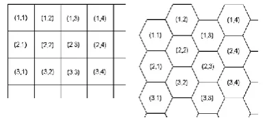
[image:2.595.63.282.326.416.2]a CA can be defined as a 4-tuplet 𝑈 = 𝑅, 𝑁, 𝑄, 𝑘 where R is the cellular space formed by a two-dimensional array of q x b cells: 𝑥, 𝑦 , 1 ≤ 𝑥 ≤ 𝑞, 1 ≤ 𝑦 ≤ 𝑏 , such that each of which can assume a state. In the bi-dimensional case, the cells are usually represented as identical square areas (Fig.2 ), but in this work, the cells will be represented by means of regular hexagonal areas (Fig. 2), making a tessellation of the plane. This new representation allows us to obtain a more realistic simulation [1].
Fig.2. Square cellular space and Hexagonal cellular space
3.2 The Cellular Automata Based Model
For Tsunami Wave Spreading
In this section the model for predicting tsunami wave spreading based on two-dimensional linear cellular automata with hexagonal cellular space is proposed. In this model ocean area can be interpreted as the hexagonal cellular space by simple dividing it into a two-dimensional array of identical hexagonal areas of side length L. Obviously, each one of these areas stands for a cell of the CA.
Fig 3. Even neighbour cells Fig.4. Odd neighbour cells The state of a cell (x,y) at a time t, is defined as follows:
𝑁𝑥𝑦(𝑡)= traversed area of (x,y) at a time t / total area of (x,y)
where as a simple calculus shows, the total area of the hexagonal cell (x,y) is 3√3L2 / 2.If 𝑁
𝑥𝑦(𝑡)= 0, then the cell
(x,y) is said to be untraversed at time t; if 0 < 𝑁𝑥𝑦(𝑡)< 1, then
the cell (x,y) is partially traversed out at time t, and finally if
𝑁𝑥𝑦(𝑡)= 1, the cell is said to be completely traversed out at time
t. Observed that the values 𝑁𝑥𝑦(𝑡)may else be greater than 1.
In this case, the state of the cell (x,y) at time t is taken to be equal to 1.
[image:2.595.325.556.403.520.2]𝑁𝑥𝑦 𝑡+1 = 𝑓 (𝑁𝑥𝑦 𝑡 + 𝜇λδ (𝑥,𝑦)
𝑁𝑥+ 𝑡 λ,𝑦+δ
λ,δ ∈𝑄𝑛
+
𝜇λδ 𝑥,𝑦 𝑁𝑥+ 𝑡 λ,𝑦+δ
λ,δ ∈𝑄𝑑
)
where 𝜇λδ 𝑥,𝑦 ∈ ℤ are parameters involving some physical magnitudes of the cells, and the discretization function f is given by
f: [0,1]→ 𝑁
𝑎 ↦ 𝑓 𝑎 = 10𝑎
10 ,
𝑤ℎ𝑒𝑟𝑒 𝑐 stands for the closest integer to c.
As it is mentioned above, each cell (x, y), represents a small hexagonal area of the ocean. Then, it is endowed with three parameters: the rate of wave spread𝑅𝐴 𝑥,𝑦 , the wave speed 𝑊𝐴 𝑥,𝑦 ), and the depth 𝐷𝐸 𝑥,𝑦 of the cell.
Consequently, the expression of the parameter 𝜇λδ 𝑥,𝑦 is as follows:
𝜇λδ 𝑥,𝑦 = 𝜔𝑎λδ 𝑥,𝑦 . 𝑑𝑒λδ 𝑥,𝑦 . 𝑟𝑎λδ 𝑥,𝑦 Where 𝑊𝐴 𝑥,𝑦 stands for the wave influence of the neighbor cell (𝑥 +λ, 𝑦 +δ)on (x,y), such that 𝑊𝐴 𝑎,𝑏 = {𝜔𝑎λδ 𝑥,𝑦 ,(λ,δ) ∈ 𝑄};𝑑𝑒λδ 𝑥,𝑦 represents
the height influence and, as is shown below, it is a function of
𝐷𝐸 𝑥,𝑦 − 𝐷𝐸 𝑥−λ,𝑦+δ where 𝐷𝐸 𝑥,𝑦 )is the height in the
central point of the hexagonal area which is represented by the cell 𝑥, 𝑦 . It is supposed that this height is the same in every point of such cell. Finally, 𝑟𝑎λδ 𝑥,𝑦 is a parameter which stands for the influence of the different rates of tsunami wave spread.
3.3 The Size of Discrete Time Step
Since cellular automata evolve in discrete time steps, it is a basic point to decide the size of such step of time𝑡 . In the proposed model, this step is equal to the time needed for a one and only near neighbor cell to be traversed.
The rate of tsunami wave spread of the cell (x,y),
𝑅𝐴 𝑥,𝑦 ,determines the time needed for this cell to be completely traversed out and depends on the physical composition of the cell [10]. Note that if the cell (x,y) stands for an untraversed hexagonal area, then 𝑅𝐴 𝑥,𝑦 =0 and 𝑁𝑥𝑦 𝑡
= 0 for every t.
The importance of this parameter lies in the setting-up of the size of the time step 𝑡 . Suppose that the ocean area modeled is homogeneous, i.e. the value of the rate of wave spread is the same for all cells :{𝑅𝐴 𝑥,𝑦 ,1 ≤ 𝑥 ≤ 𝑞, 1 ≤ 𝑦 ≤ 𝑏}
Then, it is easy to check that if the only traversed cell at time t in the neighbourhood of O is for example N, then the time needed for O to be completely traversed out is 𝑡̃ = 3𝑅𝐿 Consequently, if all cells in the neighbourhood of
𝑂 = 𝑥, 𝑦 are untraversed at time t except only one adjacent cell, which is completely traversed out, then at time t + 1, the cell (𝑥, 𝑦) is completely traversed: 𝑁𝑥𝑦 𝑡+1 =1
However, since almost all real oceans are non- homogeneous, the step size is taken to be the time needed for the cells with the larger rate spread to be completely traversed out,that is
𝑡̃ = 3𝑅𝐿 (1) where RA=max {𝑅𝐴 𝑥,𝑦 ,1 ≤ 𝑥 ≤ 𝑞, 1 ≤ 𝑦 ≤ 𝑏}
It is followed that if the only completely traversed out neighbour cell at time t, is a distant neighbour cell of O = (x,y), say NNE,then 𝑁𝑥𝑦 𝑡+1 =γ<1. That value is
calculated as follows. In a step time𝑡 , the near neighbor cells of the cell NNE, N and NE, and a little portion (a circular sector) of the cell O will be traversed out. Specifically, as the distance covered by the tsunami wave spread in t with speed R is √3L then the radius of the circular sector of O traversed out is 3𝐿 − 𝐿
As a consequence, the traversed out area of the cell O will be
𝜋 3 − 1 2𝐿22𝜋
3 2𝜋 =
4 − 2 3 3 𝜋𝐿2
So, if all neighbour cells of (a,b) are un traversed at time t, except a distant neighbour which is fully traversed out, then
𝑁𝑥𝑦 𝑡+1 = 𝛾 =
4−2 3 3 𝜋𝐿2 3 3
2 𝐿2
=8 3−1227 𝜋 ≈ 0.216 (2)
3.4 The Influence of Tsunami Wave
Another factor to be incorporated to the model is the wave speed and direction, due to their important influence to the tsunami wave spreading [7]. As was stated above, the effect of the wave on the cell O is given by the set
𝑊𝐴 𝑥,𝑦 = {𝜔𝑎λδ 𝑥,𝑦 ,(λ,δ) ∈ 𝑄};
where 𝜔𝑎λδ 𝑥,𝑦 >0, in such a way that if no wave is traversed on 𝑂 = 𝑥, 𝑦 then 𝜔𝑎λδ 𝑥,𝑦 = 1for every λ,δ ∈ 𝑉; if the wave is traversed from North to South, then the coefficients
𝜔𝑎𝑁𝑊𝑂 , 𝜔𝑎𝑁𝑁𝑊𝑂 ,𝜔𝑎𝑁𝑂, , 𝜔𝑎𝑁𝑁𝐸𝑂 , 𝜔𝑎𝑁𝐸𝑂 must be larger than the
rest of coefficients, and so on. The value of such coefficients stand for the magnitude of the wave.
3.5 The Influence of Topography
The height differences between various points in a ocean also affects to the wave spreading. As is well-known, the waves show a higher rate of spread when they descend , whereas waves show a smaller rate of spread when they ascend.The height influence of a near neighbour cell (𝑥 +λ, 𝑦 +δ) , on a cell 𝑂 = 𝑥, 𝑦 is given by 𝑑𝑒λδ 𝑥,𝑦 ,which depends on the difference of height between each pair of cells considered, that is,
𝑑𝑒λδ 𝑥,𝑦 = ∅(𝐻𝐴 𝑥,𝑦 − 𝐻𝐴 x+λ,𝑦+δ ) (3)
The function = ∅ 𝑎 , where x stands for the height difference, must be determined according to the characteristic of the tsunami, and, also, it has to satisfy the following conditions:
If 𝑎 > 0, then ∅ 𝑎 < 1 If 𝑎 = 0, then ∅ 𝑎 = 1 If 𝑎 < 0, then ∅ 𝑎 > 1
𝐷𝐸 < 𝐷𝐸 x+λ,𝑦+δ, the tsunami wave increases its rate of
spread; the second condition states that when
𝐷𝐸 𝑥,𝑦 = 𝐷𝐸 x+λ,𝑦+δ, the topography does not affect to the
tsunami wave spread; and the third condition establishes that if 𝐷𝐸 𝑥,𝑦 > 𝐷𝐸 x+λ,𝑦+δ the tsunami wave restrains its
spreading. Moreover, the height influence of a distant neighbour cell is affected by the influence of its associated near neighbour cells.
For example, if the distant neighbour cell of O is NNE, then:
𝑑𝑒𝑁𝑁𝐸𝑂 =14 ∅ 𝐷𝐸𝑂− 𝐷𝐸𝑁 + ∅ 𝐷𝐸𝑁− 𝐷𝐸𝑁𝑁𝐸 +
∅𝐷𝐸𝑂−𝐷𝐸𝑁𝐸+∅𝐷𝐸𝑁𝐸−𝐷𝐸𝑁𝑁𝐸 and so on.
Note that if the tsunami is horizontal wave motion (all cells have the same height), then ∅ 𝑎 ≤ 1 and consequently
𝑑𝑒λδ 𝑥,𝑦 = 1 for every cell (x,y) and any( λ,δ) ∈ 𝑄
3.6 The Rate of Wave Spread
Let us consider a non-homogeneous tsunami and set R the maximum rate of wave spread. Let O = (x,y) be a cell with
𝑅𝐴𝑂≤ 𝑅A. The purpose of this section is to determine the value of the parameter, 𝑞λδ 𝑥,𝑦 , which stands for the influence of the different rates of wave spread of the neighbor cells.If all neighbour cells are untraversed at time t except only one near neighbour cell of O, say for example N, then after a time step,
𝑡 the space traversed by the wave spread is given by :
𝑞 = 𝑅𝐴0𝑡 = 3𝑅𝐴𝑅𝐴𝑂𝐿 (4)
and consequently, there are two cases to be considered: When
𝑞 ≤ 𝐿 , and when q > L.
If 𝑞 ≤ 𝐿 , then 3𝑅𝐴𝑅𝐴𝑂𝐿 ≤ 𝐿 , and 𝑅𝐴𝑅𝐴𝑂≤ 33 ≈ 0.57735 As a consequence, the traversed out area of the cell O after a time step ~t is given by𝐿𝑞+ 2
𝑞2𝜋 6
2 = ( 3 + 𝜋 2
𝑅𝐴𝑂
𝑅𝐴 ) 𝑅𝐴𝑂
𝑅𝐴 𝐿2
Consequently,
𝑞𝑁𝑂=
3 +𝜋2 𝑅𝐴𝑂
𝑅𝐴 𝑅𝐴𝑅𝐴 𝐿𝑂 2 3
2 3𝐿2
=
2 3 9 3 +
𝜋 2
𝑅𝐴𝑂
𝑅𝐴 𝑅𝐴𝑂
𝑅𝐴 (5)
If 𝑞 > 𝐿, then 𝐿 < 3 𝑅𝐴𝑅𝐴𝑂𝐿,, and
0.57735 ≈ 3 3 <
𝑅𝐴𝑂 𝑅𝐴 ≤ 1
As a simple calculus shows, the traversed out area of the cell O = (x,y) after a time step 𝑡 is given by
1 + sin(π
6−λ) + 3λ 𝑅𝐴𝑂
𝑅𝐴 3 𝑅𝐴𝑂
𝑅𝐴 𝐿2
where,
λ=𝜋
6 −𝑎𝑟𝑐𝑐𝑜𝑠 (
3 4
𝑅𝐴 𝑅𝐴𝑂+
3
12 12 − 3
𝑅𝐴2
𝑅𝐴𝑜2),
0 ≤λ<𝜋 6 (6)
As a consequence:
𝑞
𝑁𝑂=
1+sin (6π−λ)+ 3λ𝑅𝐴 𝑂𝑅𝐴 3 𝑅𝐴 𝑂𝑅𝐴 𝐿2 32 3𝐿2
=23[1 + sin(π
6−λ)] 𝑅𝐴𝑂
𝑅𝐴 + 2 3
3 λ 𝑅𝐴𝑜2
𝑅𝐴2 (7)
Note that if the tsunami is homogeneous, then Rab = R for
every cell (x,y), and
λ=𝜋
6 − 𝑎𝑟𝑐𝑐𝑜𝑠(
3
2) =0 (8)
Consequently 𝑞𝑁𝑂= 1 was expected.On the other hand, if all
neighbour cells are untraversed at time t, except only one distant neighbour cell, say for example NNE, then after a time step 𝑡 , the wave spread traverses the border between the near neighbour cells N and NE, and affects the main cell O.
The border line between N and NE is traversed in 𝑡 -L/max {RAN,RANE} and consequently, the space traversed along the
cell O is:
𝑅𝐴𝑂 𝑡 − 𝑡 𝑂 = 3𝑅𝐴−max 𝑅𝐴1
𝑁,𝑅𝐴𝑁𝑁𝐸 𝑅𝐴𝑂𝐿
As a consequence, the traversed out area of O after a time step 𝑡 is:
𝜋 𝑅𝐴 −3 1 max 𝑅𝐴𝑁,𝑅𝐴𝑁𝑁𝐸
2
𝑅𝐴𝑂2𝐿22𝜋3
3 2 3𝐿2
=𝜋 3
3 𝑅𝐴−
1 max 𝑅𝐴𝑁,𝑅𝐴𝑁𝑁𝐸
2
𝑅𝐴𝑂2𝐿2 (9)
Obviously, the state of the cell O is
=
𝜋
3 𝑅𝐴 −3 max𝑅𝐴1𝑁,𝑅𝐴
𝑁𝑁𝐸 2
𝑅𝐴𝑂2𝐿2
3 2 3𝐿2
𝑞𝑁𝑁𝐸𝑂 = 2𝜋 327 ( 3𝑅𝐴𝑅𝐴𝑂− max 𝑅𝐴𝑅𝐴𝑁,𝑂𝑅𝐴𝑁𝑁𝐸 )2
Note that if the tsunami is homogeneous, then
𝑞𝑁𝑁𝐸𝑂 = 2𝜋 327 ( 3 − 1)2=8 3−1227 =γ (10)
4.
SIMULATION
RESULTS
OF
TESTING OF MODULES
4.1 Homogeneous Ocean Rate of Spread
Calculation
► Near Cells:
If 𝑞 ≤ 𝐿then, 𝑞𝑁𝑂= 2 39 3 +𝜋2 𝑅𝐴𝑅𝐴𝑂 𝑅𝐴𝑅𝐴𝑂
If 𝑞 > 𝐿 then, 1 + sin(π
6−λ) + 3λ 𝑅𝐴𝑂
𝑅𝐴 3
𝑅𝐴𝑂 𝑅𝐴 𝐿
2; where,λ =0.
► Distant Cells:
𝑞𝑁𝑁𝐸𝑂 = 2𝜋 327 ( 3 − 1)2=8 3−1227 =γ
4.2 Homogeneous Ocean, horizontal wave
motion and Primary Wave Speed
In the case of horizontal wave motion, the spread is even and with primary wave speed, the spread is even in all directions as shown in the Fig.6.
2D model Hexagonal
Fig.6. Homogeneous Ocean, horizontal wave motion for primary wave speed and all directions.
4.3 Homogeneous Ocean, horizontal wave
motion and Secondary Wave Direction
In this case, from the central cell, the neighbouring cells are partially traversed, and then they are completely traversed, in the specified direction. The spread is even andwith secondary wave direction, the spread is more in the
2D model Hexagonal Fig.7. Homogeneous Ocean, horizontal wave motion
for secondary wave speed and direction in North-West
4.4 Homogeneous Ocean, Vertical wave
motion and Primary Wave Speed
In this case of vertical wave motion, the spread is very fast in the trans-ocean tsunami direction, moderate on the sides if the slope and very slow down the slope. With primary wave speed, the spread is even as shown in the Fig.8.
2D model Hexagonal Fig.8. Homogeneous Ocean, Vertical wave motion for
primary wave speed
4.5 Homogeneous Ocean, Vertical wave
motion and Secondary Wave Speed
In this case, from the central cell, the neighbouring cells are partially traversed, and then they are completely traversed, in the specified direction.
In vertical wave motion, the spread is very fast in the trans-ocean tsunami direction, moderate in the sides of the slope and very slow down the slope. With secondary wave directions, the spread is more on the specified direction; the spread is shown in the Fig.9.
2D model Hexagonal
5 NON- HOMOGENEOUS MODULES
5.1 Non-Homogeneous Ocean, Rate of
Spread Calculation
► Near Cells: If 𝑞 ≤ 𝐿 then,
𝑞𝑁𝑂= 2 39 3 +𝜋2 𝑅𝐴𝑅𝐴𝑂 𝑅𝐴𝑅𝐴𝑂 If 𝑞 > 𝐿 then,
𝑞𝑁𝑂=23[1 + sin(π6−λ)]𝑅𝐴𝑅𝐴𝑂+2 33 λ𝑅𝐴𝑜
2
𝑅𝐴2; where,
λ=π
6− arccos( 3
4 𝑅𝐴 𝑅𝐴(𝑥,𝑦 )+
3
12 12 − 3
𝑅𝐴2
𝑅𝐴(𝑥,𝑦 )2 ),
0≤λ ≤ π/6
► Distant Cells:
𝑞𝑁𝑁𝐸𝑂 = 𝜋 3
3 𝑅𝐴−
1 max 𝑅𝐴𝑁 ,𝑅𝐴𝑁𝑁𝐸
2 𝑅𝐴𝑂2𝐿2
5.2. Non-Homogeneous Ocean, horizontal
wave motion and Primary Wave Speed
In the case of horizontal wave motion, the spread is even and with primary wave speed, the spread is even in all directions; which is shown in the Fig.10.
2D model Hexagonal
Fig.10. Non-homogenous Ocean, horizontal wave motion with Primary wave
5.3 Non -Homogeneous Tsunami, horizontal
wave
motion
and
Secondary
Wave
Direction
In this case of horizontal wave motion, the spread is even and with secondary wave direction, the spread is more in the specified direction, which is shown in the Fig.11.
2D model Hexagonal
Fig.11. Non-homogenous Tsunami, horizontal wave motion with Secondary wave speed in South-West
5.4 Non -Homogeneous Ocean, horizontal
wave
motion
and
Secondary
Wave
Direction
In the case of vertical wave motion, the spread is very fast in the trans-ocean tsunami direction, moderate in the sides of the slope and very slow down the slope. With primary wave speed, the spread is even; which is shown in the Fig.12.
2D model Hexagonal
Fig.12. Non-homogenous Ocean, Vertical wave motion with Primary wave speed
5.5 Non-Homogeneous Tsunami, Vertical
wave
motion
and
Secondary
Wave
Direction
In the case of vertical wave motion, the spread is very fast in the trans-ocean tsunami direction, moderate in the sides of the slope and very slow down the slope. With secondary wave direction, the spread is more in the specified direction; which is shown in the Fig.13.
2D model Hexagonal
Fig.13. Non-homogenous ocean, Vertical wave motion for Secondary wave speed in North-West
6
COMPARISONS
WITH
TWO-DIMENSIONAL SQUARE CELLULAR
AUTOMATA
6.1 Rate of Spread (Homogeneous Oceans)
Here the rate of spread of hexagonal cellular automata with that of Two-dimensional Square cellular automata for homogeneous tsunamis [10] with horizontal wave motions and primary wave are compared.
Fig.14. Comparison of rates of spread between Two-dimensional Square CA and Hexagonal CA in
homogeneous Ocean.
6.2
Number
of
Cells
Traversed
(Homogeneous Oceans)
Here the number of cells traversed in hexagonal cellular automata with that of two-dimensional square cellular automata for homogeneous oceans with Horizontal wave motion and primary wave are compared. It is seen that the number of cells traversed in our result is less when compared to that of the Two-dimensional Square model. This is because the area of a square cell is small, so the cells traversed at a particular time is more, when compared to the area of the hexagonal cells, which is large and hence the cells traversed at a particular time is less.
Fig.15. Comparison of no. of cells traversed between Two-dimensional Square CA and Hexagonal CA in
homogeneous Ocean.
6.3 Rate of Spread (Non-Homogeneous
Oceans)
Here the rate of spread of hexagonal cellular automata with that of Two-dimensional square cellular automata for non-homogeneous oceans with horizontal wave motions and primary wave are compared. From the graph it is seen that the rate of spread is nearly constant which is not accurate for any non-homogeneous oceans. Comparatively the rate of spread is uneven in our results, which is more compatible with the rate of spread in non-homogeneous ocean.
Fig.16.Comparison of rates of spread between Two-dimensional Square CA and Hexagonal CA in
non-homogeneous Ocean.
6.4 Number of Cells Traversed
(Non-Homogeneous Oceans)
Here the number of cells traversed in hexagonal cellular automata with that of two-dimensional square cellular automata for non-homogeneous oceans with horizontal wave’s motion and primary waves are compared. It is seen that the number of cells traversed in two-dimensional square model is more, even though the area of the cells is less. But in this result, the area of the cells is more and the number of cells traversed is less, which is more accurate.
Fig.17. Comparison of no. of cells traversed between Two-dimensional square CA and Hexagonal CA in
7. CONCLUSIONS
In this work, a multi model for the prediction of tsunami wave spreading has been introduced. It is based on the basic, two dimensional, hexagonal cellular automata and incorporates weather and wave topography conditions. The states of each cell are well defined by means of transfer of fractional traversed area. Also, different rates of speed are considered. The algorithm seems to be very efficient and is easily implemented in any computer algebra system, allowing a low computational cost.
The model is applied to eight basic cases depending on the weather, topography and wave speed conditions. All the graphical models obtained are found to be in agreement with wave spreading in real tsunamis.
8 .REFERENCES
[1] D.H.Zhang,T.L.Yip and C.-O.Ng,Predicting tsunami arrivals:Estimates and policy implications,Marine Policy,33(2009),643-650
[2] Yuri,I.S and Leonid B.Clubaror .,(1995),Mathematical modeling in mitigating the hazardous effects of tsunami waves in the ocean-a prior analysis and timely online forecast,Science of tsunami hazards 1391),pp27-44.
[3] “Offshore,Nearshore and Foreshore Behavior of Tsunami Waves”,New Mexico heigh School Adventures in Supercomputing Challenge Final Report April24,2006. [4] http://www.tsunami.noaa.gov/terminology.html
[5] Eric L. Geist2005, ,Local Tsunami Hazards in the Pacific Northwest from Cascadia Subduction Zone Earthquakes , U.S. Geological Survey Professional Paper 1661-B. [6] M. H. Dao and P. Tkalich “Tsunami propagation
modelling – a sensitivity study”Nat. Hazards Earth Syst. Sci., 7, 741–754, 2007,
[7] Wolfram,S.,(1983),Statistical Mechanics of Cellular Automata, Reviews of Modern Physics 55,601-644 [8] E.Syed Mohamed and S.Rajasekaran “Tsunami Wave
Propagation Models based on two-dimensional Cellular Automata, International Journal of Computer Applications (0975 – 8887) Volume 57, November 2012 [9] E.Syed Mohamed and S.Rajasekaran “Tsunami Wave
Propagation Models based on Hexogonal Cellular Automata(Communicated for publication)