http://dx.doi.org/10.4236/jdaip.2014.22006
User Model Clustering
Loc Nguyen
University of Science, Ho Chi Minh, Vietnam Email: [email protected]
Received 15 March 2014; revised 17 April 2014; accepted 4 May 2014
Copyright © 2014 by author and Scientific Research Publishing Inc.
This work is licensed under the Creative Commons Attribution International License (CC BY).
http://creativecommons.org/licenses/by/4.0/
Abstract
User model which is the representation of information about user is the heart of adaptive systems. It helps adaptive systems to perform adaptation tasks. There are two kinds of adaptations: 1) In- dividual adaptation regarding to each user; 2) Group adaptation focusing on group of users. To su- pport group adaptation, the basic problem which needs to be solved is how to create user groups. This relates to clustering techniques so as to cluster user models because a group is considered as a cluster of similar user models. In this paper we discuss two clustering algorithms: k-means and
k-medoids and also propose dissimilarity measures and similarity measures which are applied into different structures (forms) of user models like vector, overlay, and Bayesian network.
Keywords
User Model, Cluster
1. Introduction
User model is the representation of personal traits (or characteristics) about user, such as demographic informa- tion, knowledge, learning style, goal, interest, etc. Learner model is defined as user model in learning context in which user is a learner who profits from (adaptive) learning system. We note that learner model, student model, and user model are the same terms in learning context. Adaptive systems exploit valuable information in user model so as to provide adaptation effects, i.e., to behave different users in different ways. For example, the adaptive systems tune learning materials to a user in order to provide the best materials to her/him. The usual adaptation effect is to give individually adaptation to each user, but there is a demand to provide adaptation to a group or community of users. Consequently, all users in the same group will profit from the same learning mate-rials, teaching methods, etc. because they have the common characteristics. So there are two kinds of adaptations:
1) Individual adaptation regarding to each user;
2) Community (or group) adaptation focusing on a community (or group) of users. Group adaptation has more advantages than individual adaptation in some situations:
rela-niques so as to cluster user models because a group is considered as a cluster of similar user models. Sections 2 and 3 discuss about user modeling clustering technique, namely k-means algorithm for vector model, overlay model, Bayesian network. In Section 3, we propose formulations so as to compute the dissimilarity of two over-lay models (or two Bayesian network). The k-medoids algorithm and similarity measures such as cosine similar-ity measure and correlation coefficient are discussed in Section 4. Section 5 is the conclusion.
2. User Model Clustering Method
Suppose user model Ui is represented as vector Ui=
{
u ui1, , , , ,i2 uij uin}
whose elements are numbers. For instance, if Ui represents user knowledge then Ui is considered as a knowledge vector in which the jthcomponent of this vector is the conditional probability expresing how user master knowledge item jth. Note that Ui is called user model or user vector or user model vector.
Suppose there is a collection of users
{
U U1, , ,2 Um}
and we need to find out k groups so-called k usermodel clusers. A user model cluster is a set of similar user models, so user models in the same cluster is dissi- milar to ones in other clusters. The dissimilarity of two user models is defined as Euclidean distance between them.
(
)
(
)
(
) (
2)
2(
)
21 2 1 2 11 21 12 22 1 2
dissim U U, =distance U U, = u −u + u −u + + un−un
The less dissim(U1, U2) is, the more similar U1 and U2 are. Applying k-means algorithm [1], we partition a collection of user models into k user model clusters. The k-means algorithm (see Figure 1) includes three fol-lowing steps:
1) It randomly selects k user models, each of which initially represents a cluster mean. Of course, we have k cluster means. Each mean is considered as the “representative” of one cluster. There are k clusters.
2) For each remaining user model, the dissimilarities between it and k cluster means are computed. Such user model belongs to the cluster which it is most similar to; it means that if user model Ui belong to cluster Cj, the dissimilarity measure dissim(Ui, Cj) is minimal.
3) After that, the means of all clusters are re-computed. If stopping condition is met then algorithm is termi-nated, otherwise returning step 2.
This process is repeated until the stopping condition is met. For example, the stopping condition is that the square-error criterion is less than a pre-defined threshold. The square-error criterion is defined as below:
(
)
1 idissim
k
i i U C
Err U m
= ∈
=
∑ ∑
−where Ci and mi is cluster i and its mean, respectively; dissim(U, mi) is the dissimilarity between user model U and the mean of cluster Ci.
The mean mi of a cluster Ci is the center of such cluster, which is the vector whose tth component is the aver-age of tth components of all user model vectors in cluster C
i.
1 2
1 1 1
1 ni ,1 ni , ,1 ni
i j j jn
j j j
i i i
m u u u
n = n = n =
=
∑
∑
∑
where ni is the number of user model in cluster Ci.
3. Clustering Overlay Model
Figure 1. User model clusters (means are marked by sign “+”).
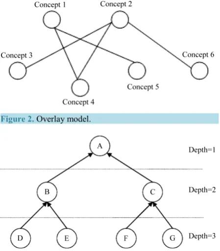
there is a question: how to compute such measure in case that user model is an overlay model which is in form of domain graph? In this situation, the domain is decomposed into a set of elements and the overlay model is simply a set of masteries over those elements. So overlay model is the subset of domain model (see Figure 2).
It is essential that overlay model is the graph of domain; so overlay model is also called as graph model. Each node (or vertex) in graph is a knowledge item represented by a number indicating how user masters such know-ledge item. Each edge (or arc) reveals the relationship between two nodes. It is clear to say that the dissimilarity measure needs changing so as to compare two overlay models. Note that the terms “user model”, “overlay mod-el”, “graph model” are the same in this context. Suppose two user overlay models U1 and U2 are denoted as be-low:
1 1 1, 1 and 2 2 2, 2
U =G = V E U =G = V E
where Vi and Ei are set of nodes and set of arcs, respectively. Vi is also considered as a vector whose elements are numbers representing user’s masteries of knowledge items.
(
1, , ,2)
i i i in
V = v v v
Suppose graph model is in form of tree in which each directed arc represents the prerequisite relationship of two nodes. If there is an arc from node A to node B, user must master over A before learning B.
Let depth(vij) is the depth level of node j of graph model Gi. Note that the depth level of root node is 1.
(
)
depth vroot =1
Given the assumption “the structure of graphs of all users is kept intact”, the dissimilarity (or distance) of two graph models G1 and G2 is defined as below:
(
)
(
)
1( )
21 2 1 2
1 1
dissim , distance ,
depth n
j j
j j
v v
G G G G
v
=
−
= =
∑
The meaning of this formulation is: the high level concept (node) is the aggregation of low level (basic) con-cepts.
The depth levels of jth nodes of all graph models are the same because the structure of graphs is kept intact.
( )
( )
, , , depth aj depth bj
a b j v v
∀ =
For example, there are three graph models whose structures are the same to the structure shown in Figure 3. The values of their nodes are shown in Table 1:
The dissimilarity (or distance) between G3 and G1, G2, respectively are computed as below:
(
)
(
)
1 3
2 3
2 2 1 1 1 1 0 1 3 4 2 5 1 4
dissim , 2.66
1 2 2 3 3 3 3
1 2 1 1 0 1 1 1 4 4 5 5 4 4
dissim , 1.5
1 2 2 3 3 3 3
G G
G G
− − − − − − −
= + + + + + + =
− − − − − − −
= + + + + + + =
So G2 is more similar to G3 than G1 is.
3.1. In Case That Arcs in Graph Are Weighted
Figure 2. Overlay model.
[image:4.595.200.400.386.465.2]Figure 3. Graph model in form of tree and prerequisite rela- tionships.
Table 1.Values of graph nodes.
A B C D E F G
G1 2 1 1 0 3 2 1
G2 1 1 0 1 4 5 4
G3 2 1 1 1 4 5 4
node and child node, the following figure shows this situation:
The dissimilarity (or distance) of two graph models G1 and G2 is re-defined as below:
(
)
(
)
1( )
2( )
1 2 1 2 1
1 1
dissim , distance , weight
depth n
j j
j
j j
v v
G G G G v
v
=
−
= =
∑
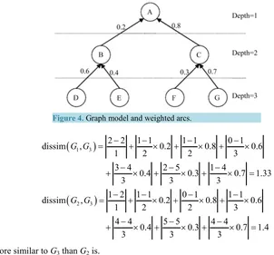
×Let weight(vij) be the weight of arc from node j (of graph model i) to its parent. We consider that weight(vij)is the weight at node vij.The sum of weights at nodes having the same parent is equal to 1.
( )
have the same parentweight 1
ij
ij
v v
=
∑
The weight at root node is equal to 1.
(
)
weight vroot =1.
The weight at jth nodes of all graph models are the same because the structure of graphs is kept intact.
( )
( )
, , , weight aj weight bj
a b j v v
∀ =
Figure 4. Graph model and weighted arcs.
(
)
(
)
1 3
2 3
2 2 1 1 1 1 0 1
dissim , 0.2 0.8 0.6
1 2 2 3
3 4 0.4 2 5 0.3 1 4 0.7 1.33
3 3 3
1 2 1 1 0 1 1 1
dissim , 0.2 0.8 0.6
1 2 2 3
4 4 0.4 5 5 0.3 4 4 0.7 1.4
3 3 3
G G
G G
− − − −
= + × + × + ×
− − −
+ × + × + × =
− − − −
= + × + × + ×
− − −
+ × + × + × =
So G1 is more similar to G3 than G2 is.
3.2. In Case That Graph Model Is Bayesian Network
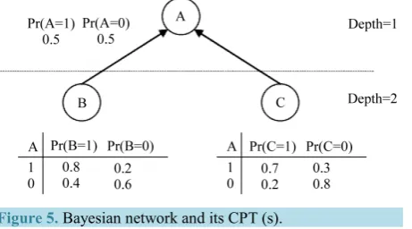
Bayesian network is the directed acrylic graph (DAG) [2] [3] constituted of a set of nodes and a set of directed arc. Each node is referred as a binary variable and each arc expresses the dependence relationship (namely, pre- requisite relationship) between two nodes. The strength of dependence is quantified by Conditional Probability Table (CPT). In other words, each node owns a CPT expressing its local conditional probability distribution. Each entry in the CPT is the conditional probability of a node given its parent. The marginal probability of a node expresses user’s mastery of such node. Note that marginal probability is considered as posterior probability.
Suppose the structure of Bayesian network is in form of tree, Figure 5 shows our considered Bayesian net-work.
Let G1 and G2 be two Bayesian networks of user1 and user2, respectively.
1 1, 1 and 2 2 2, 2
G = V E U =G = V E
where Vi and Ei are a set of nodes and a set of arcs, respectively. The dissimilarity (or distance) of two Bayesian networks G1 and G2 is defined as below:
(
)
(
)
( )
1( )
( )
21 2 1 2
1 1
dissim , distance ,
depth
n j j
j j
Pr v Pr v
G G G G
v
=
−
= =
∑
where Pr(vij) is the marginal probability of node j in network i. The inference technique to compute marginal probability is discussed in [2].
4. Similarity Measures for Clustering Algorithm
Although dissimilarity measure considered as the physical distance between them is used to cluster user models, we can use another measure so-called similarity measure so as to cluster user models. There are two typical si-milarity measures:
Figure 5. Bayesian network and its CPT (s).
Suppose user model Ui is represented as vector Ui = {ui1, ui2,…, uij,…, uin}, the cosine similarity measure of two user models is the cosine of the angle between two vectors.
(
)
(
)
12 2
1 1
, cos ,
n
ik jk
i j k
i j i j n n
i j
ik jk
k k
u u U U
sim U U U U
U U u u = = = × ⋅ = = = ⋅
∑
∑
∑
The range of cosine similarity measure is from 0 to 1. If it is equal to 0, two users are totally different. If it is equal to 1, two users are identical. For example, Table 2 shows four user models.
The cosine similarity measures of user4 and user1, user2, user3 are computed as below:
(
user ,user4 1)
2 1 1 2 2 1 02 2 2 2 2 0.91 2 0 1 2 1
sim = × + × + × =
+ + + +
(
user ,user4 2)
2 2 1 1 2 1 02 2 2 2 2 0.61 2 0 2 1 2
sim = × + × + × =
+ + + +
(
user ,user4 3)
2 4 1 1 2 5 02 2 2 2 2 0.41 2 0 4 1 5
sim = × + × + × =
+ + + +
Obviously, user1 and user2 are more similar to user4 than user3 is.
On other hand, correlation coefficient which is the concept in statistics is also used to specify the similarity of two vectors. Let Ui be the expectation of user model vector Ui.
1 1 n i ik k U u n = =
∑
The correlation coefficient is defined as below:
(
)
(
)
(
)(
)
(
)
(
)
1 2 2 1 1 , , nik i jk j
k
i j i j n n
ik i jk j
k j
u U u U
sim U U correl U U
u U u U
= = = − − = = − −
∑
∑
∑
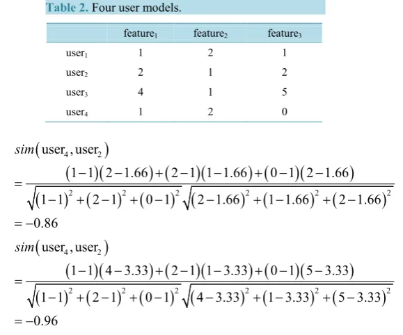
The range of correlation coefficient is from –1 to 1. If it is equal to –1, two users are totally different. If it is equal to 1, two users are identical. For example, the correlation coefficients of user4 and user1, user2, user3 are computed as below:
4 1 2 0 13
U = + + = , 1 1 2 1 1.33
3
U = + + = , 2 2 1 2 1.66
3
U = + + = , 3 4 1 5 3.33
3 U = + + =
(
)
(
)(
) (
)(
) (
)(
)
(
) (
) (
) (
) (
) (
)
4 1 2 2 2 2 2 2
1 1 1 1.33 2 1 2 1.33 0 1 1 1.33
user ,user 0.86
1 1 2 1 0 1 1 1.33 2 1.33 1 1.33
sim = − − + − − + − − =
Table 2.Four user models. feature1 feature2 feature3 user1 1 2 1 user2 2 1 2 user3 4 1 5 user4 1 2 0
(
)
(
)(
) (
)(
) (
)(
)
(
) (
) (
) (
) (
) (
)
4 2
2 2 2 2 2 2
user ,user
1 1 2 1.66 2 1 1 1.66 0 1 2 1.66
1 1 2 1 0 1 2 1.66 1 1.66 2 1.66
0.86
sim
− − + − − + − −
=
− + − + − − + − + −
= −
(
)
(
)(
) (
)(
) (
)(
)
(
) (
) (
) (
) (
) (
)
4 2
2 2 2 2 2 2
user ,user
1 1 4 3.33 2 1 1 3.33 0 1 5 3.33
1 1 2 1 0 1 4 3.33 1 3.33 5 3.33
0.96
sim
− − + − − + − −
=
− + − + − − + − + −
= −
Obviously, user1 and user2 are more similar to user4 than to user3.
If cosine measure and correlation coefficient are used as the similarity between two user vectors, the serious problem will occurs. That is impossible to specify the mean of each cluster because cosine measure and correla- tion coefficient have different semantic from Euclidean distance. Instead of using k-mean algorithm, we apply k-medoid algorithm [1] into partitioning a collection of user models into k user model clusters. The “mean” is replaced by the “medoid” in k-medoid algorithm. The medoid is the actual user model and its average similarity to all other user models in the same cluster is maximal (see Figure 6).
1) It randomly selects k user models as k medoids. Each medoid is considered as the “representative” of one cluster. There are k clusters.
2) For each remaining user model, the similarities between it and k medoids are computed. Such user model will belongs to cluster Ci if the similarity measure of this user model and the medoid of Ci is the highest.
3) After that, k medoids are selected again so that the average similarity of each medoid to other user models in the same cluster is maximal. If k medoids aren’t changed or the absolute-error criterion is less than a pre-de- fined threshold, the algorithm is terminated; otherwise returning Step 2.
Figure 7 is the flow chart of k-medoid algorithm modified with similarity measure:
The absolute-error criterion which is the typical stopping condition is defined as below:
(
)
(
)
1 i 1
k
i i U C
Err sim U medoid
= ∈
=
∑ ∑
− −where Ci and medoidi is cluster i and its medoid, respectively; sim(U, medoidi) is the similarity of user model U and the medoid of cluster Ci.
5. Conclusions
We discussed two clustering algorithms: k-means and k-medoids. It is concluded that the dissimilarity measures considered as distance between two user models are appropriate to k-means algorithm and the similarity mea- sure, such as cosine similarity measure and correlation coefficient are fit to k-medoids algorithm. The reason is that the essence of specifying the mean of cluster relates to how to compute the distances among user models. Conversely, the cosine similarity measure and correlation coefficient are more effective than distance measure because they pay attention to the direction of user vector. For example, the range of correlation coefficient is from –1,“two users are totally different” to 1, “two users are identical”.
Figure 6. k-medoid algorithm (user model vectors considered as medoids are marked by sign “+”).
Figure 7. Flow chart of k-medoid algorithm.
compute the dissimilarity of two overlay models (or Bayesian network) are the variants of distances between user models.
References
[1] Han, J.W. and Kamber, M. (2006) Data Mining: Concepts and Techniques. Second Edition, Elsevier Inc., Amsterdam. [2] Nguyen, L. and Phung, D. (2009) Combination of Bayesian Network and Overlay Model in User Modeling.
Proceed-ings of 4th International Conference on Interactive Mobile and Computer Aided Learning (IMCL 2009), 22-24 April 2009, Amman.
[image:8.595.222.403.122.426.2]