An Accurate Dead Reckoning Method based on
Geometry Principles for Mobile Robot Localization
Ziyad T. Allawi
College of Education forHumanitarian Studies, University of Baghdad, Iraq
Turki Y. Abdalla
Department of Computer Engineering, College of Engineering, University of Basrah, Iraq
ABSTRACT
In this paper, an accurate method of updating the configuration pose (dead reckoning) for differential drive mobile robot localization is introduced. This method is based on the principles of geometry. This method ensures the most accurate and fast position updating in comparison with the conventional methods of configuration updating. This method was applied on a group of mobile robots in an indoor environment searching for a target.
KEYWORDS
Dead Reckoning, Geometry, Localization, Navigation, Mobile Robots.
1.
INTRODUCTION
One of the localization most and simple important techniques is the dead reckoning. This technique estimates the next robot location as a function of time using the current location and other commands like output velocity and steering. Dead reckoning varies according the design of the mobile robot. In the case of differential drive mobile robot (DDMR) which has two individual wheels on common axle, the robot should follow arc curves around a point lies on the wheel common axle [1] provided that the two wheels are fixed and have a fixed and flat contact with the ground.
In the ideal circumstances, this method is sufficient to locate the differential drive mobile robot in any next time. However, some real events may challenge this ideal situation like modeling errors, actuator command difference, wheel slipping etc. So, other pose estimation techniques are required to fix the pose estimation by Dead Reckoning especially for long-time run.
One of the important effects of odometric errors is the limited resolution during integration. This effect concerns with limited time increments and distance measurement resolutions [2]. This effect occurs when the time period T is inconsistent with the possible change of motion commands which makes the robot driven away on its real position. Another effect is the flatness of the ground. If the ground is not flat, a slip may occur and the robot misleads its way.
Although there are advanced ways of localization like using maps or GPS or using SLAM technique, dead reckoning is the most favorable technique in indoor environments [3]. Dead reckoning method used for mobile robot localization was extracted from the kinematic equation of motion. Discrete methods were used in terms of time steps to predict the next pose. One of these methods was presented in [3] and the other by [4] which is more accurate. In this article an improvement was performed on the localization method to become more
accurate. The proposed method is little more complicated than the method in [4] but is more accurate and suitable for real-time mobile robot navigation. This method can be applied on the real robots if flatness of the ground is guaranteed with no slipping, also if the robot has low speed and moves in an indoor environment.
This article is divided to some section. The second one is for theory research. It contains the three methods of dead reckoning including the proposed one. The third one is the design section which contains the design of mobile robot and its maximum speed and input wheel speeds. In the fourth section which contains the results and discussion, a comparison is held among the three methods as well as a robot simulation to illustrate the effect of this proposed method. In that simulation, this method is used to guide the robots to a found target until they reach and gather around it.
2.
RESEARCH METHOD
In this section, three methods of robot dead reckoning will be explained. The first one is the ideal method which includes the integration of the kinematic equation; the second is the approximated method which is mentioned in [2]; and the third is the method proposed in this article.
2.1
The Ideal Method:
The kinematic model of the DDMR is as follows:
sin
cos
v
y
v
x
…(1)
The output configuration vector contains the Cartesian coordinates of the DDMR in the global reference frame (x and y) as well as the orientation θ; whereas v and ω are the input linear and angular velocities of the DDMR which are used to calculate the configuration vector. To integrate the system of ordinary differential equations continuously, the orientation parameter is calculated first, and then it is used to calculate the Cartesian coordinates as in the next system of integrations:
dt
t
t
v
t
y
dt
t
t
v
t
x
dt
t
t
)
(
sin
)
(
)
(
)
(
cos
)
(
)
(
)
(
)
(
…(2)
system to be discrete. Therefore an approximate method will be used to overcome this problem.
2.2
The Approximate Method:
This method was introduced by [4] and mentioned in [2]. This method calculates the next configuration q(t+T) vector using the current vector q(t) and the current linear an angular velocities v and ω which are fixed scalars during the time period T.
The calculation method is also begins with the orientation θ which is directly calculated by the next formula:
)
(
)
(
t
T
t
T
…(3)
Then, the Cartesian coordinates x and y are then calculated using the kinematic model, where the orientation used in this calculation is the average of the current and the next orientation values:
)
2
/
)
(
sin(
)
(
)
(
)
2
/
)
(
cos(
)
(
)
(
t
s
t
y
T
t
y
t
s
t
x
T
t
x
vT
s
…(4)
This method is very useful to calculate the next configuration vector due to its simplicity and fast calculation. However, this method treats all robot tracks as linear although the actual tracks are circular most of the time. This method accumulates error over time which makes the robot diverges away from its actual position.
Therefore, it is essential to take the circular paths into account to make the computation more accurate, an that’s will be carried out in the proposed method
2.3
The Proposed Method:
This method is based on two facts related to the DDMR; which are:
The DDMR either moves in a straight line or rotates around itself or in a circular arc; because the linear and angular velocities are linearly dependant on the angular velocities of the wheels; and
The angular velocity command for the robot’s wheels is fixed through a predefined time period T.
The linear and angular velocities of the DDMR can be calculated through this matrix equation:
l r
l
l
r
v
1
1
1
1
2
…(5)
Where r is the wheel’s radius and l is the half distance between the two wheels
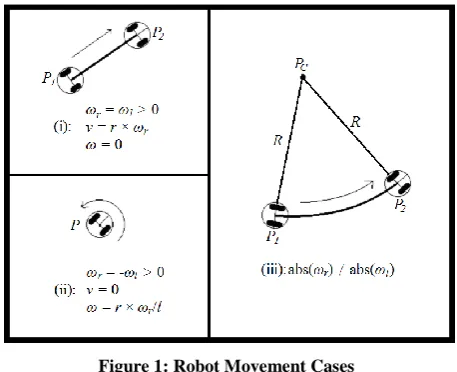
It can be seen that when the angular velocities of the right and left wheels, ωr and ωl respectively are equal, the angular velocity of the DDMR ω becomes zero (i.e. the robot is moving in a straight line; forwards or backwards); and the linear velocity v can be simply calculated by multiplying the wheel angular velocity by the wheel radius.
When the angular velocities of the DDMR wheels differ, the robot will no longer move in straight line; the robot will move in a circular path which its center C is located somewhere in
the global reference frame. The circle center C is always positioned on the line which passes the robot wheels through its axle. The position of the center my be on one of the wheels (if the angular velocity command on that wheel is zero), or it may be on the robot axle (if the angular velocity command of one wheel is positive and the other one is negative), or it may be on the center of the robot (if the two angular velocity commands are equal in magnitude and opposite in signs); in this case, the linear velocity of the robot will be zero and the robot rotates around itself like the Earth does in its daily motion.
[image:2.595.315.544.243.429.2]Fig. 1 illustrates the three possible cases of robot movement. The first two cases, (i) and (ii), are simpler in calculation than the third one (iii).
Figure 1: Robot Movement Cases
The next configuration vector of the DDMR q(t+T) can be calculated from the current configuration vector of the DDMR q(t), provided that the angular velocity values for the DDMR wheels ωr and ωl are fixed through a time period T. The calculation occurs in three cases:
Case (i) (ωr = ωl): In this case, the two angular velocity commands are equal; so the angular velocity of the robot is zero and the heading of the DDMR does not change. The linear velocity v is calculated by Eq. (5), and then multiplied by T to obtain the travelled distance Δs which can be used to update the configuration vector of the DDMR as in the equations below:
)
(
sin
)
(
)
(
)
(
cos
)
(
)
(
)
(
)
(
T
t
s
t
y
T
t
y
T
t
s
t
x
T
t
x
t
T
t
vT
s
…(6)
)
(
)
(
)
(
)
(
)
(
)
(
t
y
T
t
y
t
x
T
t
x
t
T
t
T
…(7)Case (iii) (abs(ωr) ≠ abs(ωl)): In this case, neither v nor ω are zeros; so the robot will move in a circular path around a center point which is located in a distance R away from the center of the robot. To update the configuration vector, the value of R should be calculated first, and then the coordinates of center of robot’s circular path C is found.
To prove that the track of the robot is circular, the curvature of the robot path should be calculated geometrically by this equation:
s
Curvature
…(8)The curvature is constant through T because the linear and angular velocities are made fixed. Therefore the curve which the robot takes is circular and it is possible to find the length of the circle radius R using the equation below:
v
T
vT
s
Curvature
R
1
…(9)Then, the coordinates of the center point [xC, yC] can be geometrically calculated in terms of the current and next configuration vectors: ) ( sin ) ( ) ( sin ) ( ) ( cos ) ( ) ( cos ) ( T t R T t y t R t y y T t R T t x t R t x x C C
…(10)
Finally, after some rearrangements, the important set of equations which are useful to update the configuration vector of the DDMR through the third case of robot movement can be obtained.
))
(
cos
)
(
(cos
)
(
)
(
))
(
sin
)
(
(sin
)
(
)
(
)
(
)
(
t
T
t
R
t
y
T
t
y
t
T
t
R
t
x
T
t
x
T
t
T
t
v
R
…(11)It can be seen that the system of equations above is little more complex than the approximate method in the previous section in Eq. (3) and (4).
This system of equation can also be deduced from the ideal integration system in Eq. (2). For instance, the next y-axis coordinate value can be obtained by integrating with respect to θ instead of t as follows:
( ) ) ( ) ( ) (cos
)
(
)
(
sin
)
(
)
(
)
(
)
(
sin
)
(
)
(
)
(
)
(
)
(
sin
)
(
)
(
)
(
T t t T t t T t t T t tR
t
y
T
t
y
d
R
t
y
T
t
y
dt
t
t
t
t
v
t
y
T
t
y
dt
t
t
v
t
y
T
t
y
…(12)The result is similar to the result obtained in Eq. (11). The same manner can be used in the next x-axis coordinate value. This method is also useful in calculation of total odometry (s).
3.
DESIGN PROCEDURE
The three methods were modeled using MATLAB® software using robot model which has r = 5 cm, l = 10 cm, angular velocity values of the right and left wheels ωr and ωl are -20 through 20 rad/s.
MATLAB function ode45() was used for solving ordinary differential equations in the system of Eq. (1) in discrete form, because the continuous form is not practical for digital machines. However, the other two methods were coded in simple MATLAB .m script files.
Two different angular velocities were applied upon the right and left wheels. These velocities were applied on all the methods to check their efficiencies; the error in distance and time taken in manipulation were measured to check the accuracy and speed.
The applied angular velocities in continuous form were:
1
0
)
2
sin(
20
)
(
)
2
cos(
20
)
(
t
t
t
t
t
l r
…(13)The applied angular velocities in discrete form were:
1
,
)
2
sin(
20
)
(
)
2
cos(
20
)
(
nT
N
n
nT
n
nT
n
l r
…(14)4.
RESULTS AND DISCUSSIONS
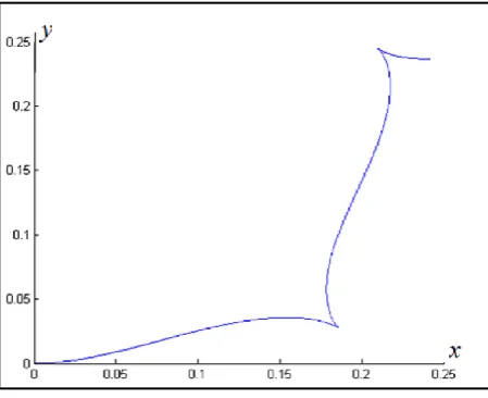
[image:3.595.317.542.511.694.2]The test was performed onto different values of T with zero initial configurations. Figure 2 shows the original track; Figures 3 and 4 show the responses of the ideal discrete form as well as the two methods for time step of 0.2 and 0.02 second respectively.
Figure 3: Response of the three methods for T = 0.2 second.
Figure 4: Response of the three methods for T = 0.02 second.
[image:4.595.54.282.302.480.2]Table I shows the computation time and distance error for each of the approximated and proposed method with respect with the discrete ideal method.
Table 1: Total Time and Distance Error for Different values of T
T Disc. Ideal Approx. Proposed Time Time Error Time Error
0.2 30 ms 140 μs 0.039 200 μs 0 0.1 60 ms 200 μs 0.013 280 μs 0 0.05 100 ms 260 μs 0.005 350 μs 0 0.02 250 ms 520 μs 0.002 660 μs 0 0.01 470 ms 1.1 ms 0.001 1.3 ms 0
Fig. 2 shows the continuous ideal track of the mobile robot. This track can be achieved if the time sample T approaches
zero. That’s clear in the Fig. 4 when the track shape approaches the ideal shape in Fig. 1.
As it stated earlier, the ideal continuous form is not practical so the discrete one was used instead. The path color of the discrete ideal curve which the mobile robot follows is black, the red dots represent the approximated method, whereas the blue dots represent the proposed method. The blue dots are coincided over the mobile robot track as shown in Figures 3 and 4. This means that the two methods (discrete ideal and proposed) are identical. This result is cited by Eq. (12) and the error column of the proposed method in Table I which hold just zeros.
Table I holds the execution times of the three methods. The first method time is much greater than the times of the other two methods; because of the complicated mathematics for solving the ordinary differential equations. This method is not practical for real-time applications because it consumes time. As it can be seen, it is useless after T = 0.05 because the computation time will be greater than T after that value. So, this type of solution is mostly discarded from use.
If a comparison occurs between the approx. and proposed methods, it can be seen that the two methods have close execution time. Although the approximated method is faster than the proposed method, but that does not exceed 20% from the speed of the proposed one. This is because latter method is little complicated than the former one.
However, in all cases, the error decreases when T becomes smaller and smaller. But the computation time should be at most 10% from T so as to let the remaining time for other Mobile Robot processes.
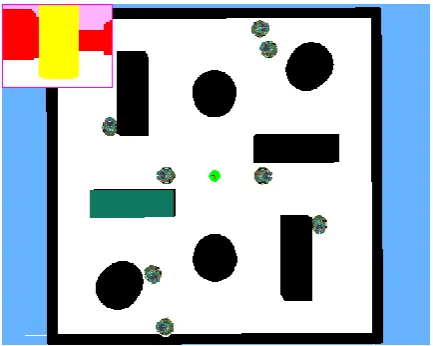
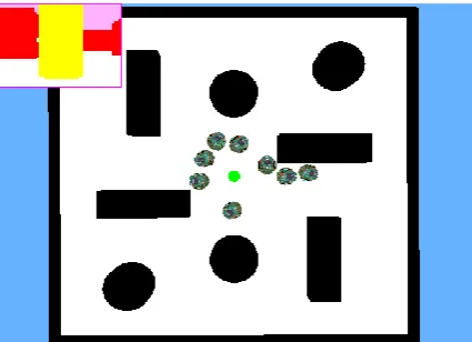
The proposed method was used in simulation of eight mobile robots searching for a target. The mobile robots used were E-puck robots [5] and the simulation was performed by Webots™ robot simulation software [6]. The robots begin their journey searching for a colored target in the middle of the environment. When one of the robots finds the target, it stops and informs other robots about its location. All robots then direct to that location until they gather around the target. Figure 5 shows the robots when they are wandering. Figure 6 shows the robots when the head to the target after they were informed about its location. Figure 7 shows the robots when they are gathering around the target.
[image:4.595.316.533.557.730.2] [image:4.595.58.276.608.730.2]Figure 6: Robots when they head to the target
Figure 7: Robots when they are gathering around the target
5.
CONCLUSIONS
It can be concluded from this work that the proposed method has succeeded in representing the discrete ideal localization method with computation time close to the fast approximated method. These features elect the proposed method to be used in real-time robot mobile localization efficiently. This method idea can inspire the derivation of localization systems for other types of mobile robots like unicycle and car-like robots.
6.
REFERENCES
[1] Siciliano, B. and Khatib, O. (Eds.), Springer Handbook of Robotics, Springer-Verlag Berlin Heidelberg, Germany, 2008.
[2] Siegwart, R. and Nourbakhsh, I. R., Introduction to Autonomous Mobile Robots, MIT Press, Cambridge, UK, 2004.
[3] Corke, P., Robotics, Vision and Control, Springer Tracts in Advanced Robotics, Springer-Verlag Berlin Heidelberg, Germany, 2011.
[4] Chong, K.S., Kleeman, L., “Accurate Odometry and Error Modeling for a Mobile Robot,” in Proceedings of the IEEE International Conference on Robotics and Automation, Albuquerque, NM, 1997.
[5] Mondada, F. and et al, “The E-puck, a Robot Designed for Education in Engineering,” In Proceedings of the 9th Conference on Autonomous Robot Systems and Competitions, Castelo Branco, Portugal, Vol. 1, No. 1, 2009, pp. 59-65.
[image:5.595.56.269.279.433.2]