Georgia State University
ScholarWorks @ Georgia State University
Real Estate Dissertations Department of Real Estate
8-9-2016
Three Essays on the Housing Market
Patrick S. SmithGeorgia State University
Follow this and additional works at:https://scholarworks.gsu.edu/real_estate_diss
This Dissertation is brought to you for free and open access by the Department of Real Estate at ScholarWorks @ Georgia State University. It has been accepted for inclusion in Real Estate Dissertations by an authorized administrator of ScholarWorks @ Georgia State University. For more information, please [email protected].
Recommended Citation
THREE ESSAYS ON THE HOUSING MARKET
BY
PATRICK STOCKDALE SMITH
A Dissertation Submitted in Partial Fulfillment of the Requirements for the Degree
Of
Doctor of Philosophy
In the Robinson College of Business
Of
Georgia State University
GEORGIA STATE UNIVERSITY ROBINSON COLLEGE OF BUSINESS
Copyright by
PATRICK STOCKDALE SMITH
ACCEPTANCE
This dissertation was prepared under the direction of Patrick Smith’s Dissertation Committee. It has been approved and accepted by all members of that committee, and it has been accepted in partial fulfillment of the requirements for the degree of Doctor of Philosophy in Business Administration in the J. Mack Robinson College of Business of Georgia State University.
Richard Phillips, Dean
DISSERTATION COMMITTEE
Dr. Jon Wiley (Chair) Dr. Karen Gibler Dr. Vincent Yao
ABSTRACT
THREE ESSAYS ON THE HOUSING MARKET
BY
PATRICK STOCKDALE SMITH
JULY 14, 2016
Committee Chair: Jon Wiley
Major Academic Unit: Department of Real Estate
Essay 1: Institutional Investment, Asset Illiquidity, and Post-Crash Housing Market Dynamics
Abstract: I demonstrate that housing’s mildly segmented market structure adds an additional measure of asset illiquidity risk for owner-occupiers and their lenders by examining the effect of a house’s conversion from the owner-occupied market to the rental market. From 2012 to 2014, I find that owner-occupied houses that were purchased by institutional investors and converted to rentals after the real estate crisis sold for approximately 5% less than similar houses that sold to owner-occupiers. The large discount was in addition to REO, foreclosure, short sale, and cash purchase discounts which, when combined, highlight the low liquidation value for owner-occupied housing.
Essay 2: Homeownership: An examination of its effect on house prices
Abstract: Subsidizing homeownership is only justifiable if it increases homeownership attainment and creates external benefits that outweigh their costs. Using parcel-level panel data I isolate and examine the effect of homeownership on surrounding house prices. Homeownership has a causal effect on house prices, but substantial variation exists across quantiles. Changes in homeownership have a lesser (greater) effect on house prices in the upper (lower) deciles of the conditional house price distribution - despite the fact that households in the upper deciles are the primary beneficiaries of the federal tax subsidies for
homeownership.
Essay 3: School Quality, Latent Demand, and Bidding Wars for Houses
Institutional Investment, Asset Illiquidity,
and Post-Crash Housing Market Dynamics
Patrick S. Smith Georgia State University
Real Estate Department
June 21, 2016
Abstract
1
1. Introduction
In the United States, there are two housing markets: owner-occupied and rental housing.
Owner-occupied housing, by definition, must be a household’s primary residence to qualify for
preferential tax treatment.1 Thus, owner-occupied housing is not only a consumption good but an
investment as well. In contrast, rental housing is not purchased for personal consumption; it is
viewed solely as an investment. The two housing markets are similar, in that, they provide
housing services. However, comparisons of the two are difficult because of housing’s mildly
segmented market structure.
Liu, Grissom and Hartzell (1990) show that single-family housing has a mildly segmented
market structure.2 Housing is a mildly segmented market because while individuals can invest in
both owner-occupied and rental housing, institutional investors can only invest in rental
housing.3 For individuals, the segmented demand results in an additional measure of risk and
hence a higher return for owner-occupied housing.4 Until recently, institutional investors have
not invested in single-family houses arising in part from high transaction costs, lack of
economies of scale (e.g. buying houses in bulk at a discount and property management issues),
and perceived political implications.5 Adverse political implications include, but are not limited
to, fear of government regulation and negative publicity regarding bidding wars with potential
homeowners given the political focus on subsidizing homeownership. Additionally, buying too
1
Homeowners can deduct property tax and mortgage interest payments for their primary residence and a second home. However, the overwhelming majority (greater than 90%) of homeowners in the United States only own one personal residence. A detailed overview of owner-occupied and rental housing’s taxation is provided in Section 3.
2
Liu, Grissom and Hartzell (1990) examine the impact of a mildly segmented housing market in a CAPM context. The authors segment the housing market into owner-occupied housing and income-producing real estate, but do not consider taxes in an effort to reduce their model’s complexity.
3
Technically institutional investors can invest in owner-occupied housing in several ways. They can purchase owner-occupied houses and hold them as dealer (or investment) properties – in which case they cannot depreciate the asset over time and do not benefit from owner-occupied housing’s preferential tax treatment, so their return is tied directly to the house’s capital appreciation. Institutional investors can also purchase owner-occupied houses and convert them rentals – in which case they are no longer owner-occupied housing. Historically, institutional investors have not invested in the equity of owner-occupied housing and instead chose to lend equity to owner-occupiers. I discuss the mildly segmented housing market and its impact on institutional investment in owner-occupied housing in greater detail in Section 2.
4
Stein (1995) shows that an exogenous negative shock to owner-occupied house prices coupled with the market’s down-payment requirements can have self-reinforcing effects. I show that these self-reinforcing effects coupled with owner-occupied housing’s preferential tax treatment, high transaction costs, and mildly segmented market structure can result in low liquidation values.
5
2
many houses in a neighborhood could change quality of life dynamics. However, the financial
crisis created a potential arbitrage opportunity for institutional investors to enter the
single-family housing market. House price declines, to levels which were significantly below their
pre-crisis levels, together with large scale delinquencies and defaults, an increase in demand for
single-family rental homes arising from these foreclosures, and the tightening of the mortgage
market created a large supply of available owner-occupied housing which made economies of
scale possible.
The purpose of this paper is to empirically examine the nature of the mildly segmented
housing market given the recent entry by institutional investors. Ex-ante, as the single-family
housing market becomes more integrated, the price of single-family homes should be bid up and
returns should fall until no abnormal returns exist if the single-family housing market becomes
fully integrated. However, segmentation might still exist due to, among other things, the
preferential tax treatment associated with owner-occupied housing. As such, I explore how the
entry of institutional investors influenced house prices by comparing the pre- versus post-crisis
period using characteristic and propensity score matched samples in a difference in difference
framework. The price differential I find provides an estimate of the asset illiquidity risk inherent
in the owner-occupied housing market that is a byproduct of the mildly segmented market
structure and the preferential tax treatment for owner-occupied housing. I also find that although
institutional investors entrance in the post-crisis period increased prices thereby reducing returns
and lessening the degree of housing market segmentation and asset illiquidity risk, the premium
associated with owner-occupied housing persists.
This study focuses on institutional investment in the Atlanta, Georgia metropolitan
housing market. Atlanta is the ideal setting for this study as it was one of the markets heavily
targeted by institutional investors (Federal Reserve Bank of Atlanta 2013; Mills, Milloy, and
Zarutskie 2015). I identify eleven institutional investors that were active in Atlanta from 2012 to
2014 – six of which were private equity firms and five of which were publicly traded
companies.6 The institutional investors that I identify are large “informed” financial entities that
entered the Atlanta housing market, purchased single-family detached houses, and converted the
houses to rentals during the post-crisis period. The institutional investors’ large cash reserves and
access to capital give them an advantage over investors that require mortgage financing in the
6
3
housing market – especially during times of economy-wide distress. In my model, institutional
investors substitute their investments in rental housing with investments in owner-occupied
housing. However, when institutional investors purchase owner-occupied housing they convert it
to rental housing for the short-term, as they cannot consume its services and can only invest in
income-producing real estate. Although housing stock is generally considered perfectly inelastic
to downward demand shocks, I show that the housing market’s mildly segmented market
structure allows owner-occupied housing to be redeployed as rental housing. In doing so, I
illustrate the impact the mildly segmented market structure has on owner-occupied housing’s
asset illiquidity and the two housing markets’ risk-return equilibrium condition.
The next section of this paper details housing’s mildly segmented market structure.
Section 3 provides an overview of owner-occupied housing’s preferential tax treatment. Section
4 applies Shleifer and Vishny’s (1992) asset liquidity framework to the owner-occupied housing
market. Section 5 presents a model of post-crash housing market dynamics, Section 6 provides
an overview of the data, Section 7 presents the empirical methodology and results, and Section 8
concludes.
2. Mildly Segmented Market Structure
There are several factors that contribute to housing’s mildly segmented market structure
including its (1) preferential tax treatment of owner-occupied housing, (2) dual role as a
consumption and investment good, (3) heterogeneous housing stock, (4) differing economies of
scale, and (5) illiquidity.
The United States government heavily subsidizes and promotes homeownership by
providing preferential tax treatment for owner-occupied housing. Owner-occupiers benefit from
the tax exemption of their implicit rental income and the exclusion of capital gains from the sale
of their house. They can also deduct their mortgage interest, mortgage insurance premium, and
property tax payments when filing their federal income taxes. The preferential tax treatment
promotes homeownership, increases owner-occupier’s consumption demand, and results in
higher house prices. In essence, preferential tax treatment for owner-occupied housing increases
owner-occupied house prices to a level that is prohibitively high for institutional investors,
thereby restricting them from entering the market.7
7
4
Housing has a dual role as both a consumption and investment good. The majority of
owner-occupiers satisfy their consumption and investment demand for housing by owning only
their primary residence without relying on the rental market to disentangle the two. Several
studies show that owner-occupier’s optimal level of housing as a consumption good often differs
from its optimal level as an investment good (Henderson and Ioannides 1983; Brueckner 1997;
Flavin and Yamashita 2002). As a result, owner-occupied housing is often “overdetermined” in
homeowner’s portfolios. The extent to which it is overdetermined is likely exacerbated by its
preferential tax treatment.
Preferential tax treatment coupled with owner-occupied housing’s dual role as a
consumption good results in a heterogeneous housing stock. Housing’s heterogeneous stock adds
to the two markets’ degree of segmentation as owner-occupiers and institutional investors’
property type and size preferences differ according to their prevailing motives (consumption
versus investment). The housing market’s stock can be split into three property types:
single-family detached, single-single-family attached, and multi-single-family housing. In theory, one could argue
that the property types are interchangeable and perfect substitutes, as single-family attached and
multi-family units are adaptive and can be redeployed (i.e. apartment buildings can be converted
into condos and vice-versa), and owner-occupied single-family detached units can easily be
converted into rentals. However, in reality, the motives of the housing market’s participants
(consumption versus investment) result in different property type preferences that are not perfect
substitutes. For example, single-family detached units are usually owner-occupied, while rental
housing is more likely to be a part of a multi-family building.
Previous research on conversion activity in housing markets has focused on condo
conversions. An increase in condo conversions - from rental housing to owner-occupied housing
- has been tied to an increase in the number of households without children (Sternlieb and
Hughes 1975), rent controls (Sternlieb and Hughes 1975;Werczberger 1988), barriers to
ownership in the single-family market (Sternlieb and Hughes 1975), tax considerations
(Whinihan 1984), reduced profitability in the rental market relative to the “for sale” market
(Diskin and Tashchian 1984; Crone 1988; Benjamin et al. 2008; Wiley 2009), low interest rates
5
(Benjamin et al. 2008; Wiley 2009), and a growing demand for homeownership (Lea and
Wasylenko 1983). The studies show that multi-family properties are valued differently in rental
and owner-occupied housing markets over time and that the property owners maximized their
return by converting rental housing to owner-occupied housing during boom periods. This study
is similar, in that, I examine housing unit conversions. However, this study focuses on
heterogeneous single-family detached houses that were converted from owner-occupied to
rentals during the recent real estate crisis.
Rental housing is more likely to be part of a multi-family building from an institutional
investors’ perspective because they look to create economies of scale. Multi-family housing
offers several advantages over single-family detached housing in this regard. Multi-family
housing, by definition, includes multiple separate housing units within one building or several
buildings in a single complex. Thus, institutional investors can purchase a large number of units
in a single transaction. Multi-family housing units are also spatially concentrated, making them
easier and cost-effective to manage, and typically have similar layouts and components, which
helps minimize repair and replacement costs as parts can be purchased in bulk. Single-family
detached housing units, in contrast, are generally not available for bulk purchase at a cost
effective price point, making it difficult for investors to accumulate a large portfolio of houses in
a short amount of time (i.e. the market has historically lacked economies of scale).8
Single-family detached housing units are also spatially dispersed and more likely to have dissimilar
layouts and components.
In addition to the differences between owner-occupiers and institutional investors
highlighted above, clientele effects exist within the two groups. For example, when looking to
purchase a house, local school quality is one of the primary considerations for owner-occupiers
with children. Whereas, owner-occupiers who do not have school age children may not be as
concerned with school quality. The size of the household plays a major role in the type of
8
6
property owner-occupiers purchase. Single-family detached housing generally offers more living
area and bedrooms, so it attracts large households.
Real estate is notoriously illiquid. In this paper I consider two types of illiquidity in
owner-occupied housing markets: market illiquidity and asset illiquidity. I define market illiquidity as
the inability to sell an owner-occupied house quickly at its full market value. Market illiquidity
in housing, similar to most real estate, is a product of the market’s high transaction costs, search
costs, and down-payment requirements. Grossman and Laroque (1990) illustrate the impact of
transaction costs on the liquidity of durable goods. In their model, households continuously
consider whether to reoptimize their level of housing consumption in relation to changes in their
wealth. They find that small transaction costs can make consumption changes occur very
infrequently.9 Stein (1995) develops a model which illustrates the self-reinforcing effect of
down-payment requirements on falling house prices. He shows that a decrease in house price
reduces homeowner’s equity; thereby reducing the amount of money the homeowner has for a
down-payment should they sell their current house. 10 A reduction in down-payment reserves
reduces household mobility and the demand for owner-occupied housing. The reduced demand
reinforces the decrease in house prices and explains housing’s illiquidity in down markets.
Housing’s degree of illiquidity varies across housing submarkets and property types, as
only the capital appreciation component of housing, and not the income producing component, is
subject to the illiquid nature of the market. The illiquid nature of owner-occupied housing has
historically made rental housing’s income-producing component more attractive to institutional
investors. Additionally, although institutional investors can lend the equity for owner-occupied
housing, they cannot directly invest in owner-occupied housing which provides income in the
form of rental opportunity costs (Liu, Grissom and Hartzell 1990). Thus, market illiquidity
reinforces the mildly segmented market structure.
Shleifer and Vishny (1992) define asset illiquidity as the difference between an asset’s
value in best use and its liquidation value. They argue that when firms are in financial distress
their industry peers are likely in a similar situation, which leads to asset sales below their value
in best use. When the housing market is in equilibrium, the best use for owner-occupied housing
9
Using a transaction cost of five percent, Grossman and Laroque estimate the average time between house purchases is 20 to 30 years. Five percent is a conservative estimate of transaction costs in housing markets as real estate broker’s commissions usually exceed five percent on their own.
10
7
is owner-occupancy and institutional investors, who value housing services based on their rental
value, are constrained from investing in owner-occupied housing. The reduced demand results in
an additional measure of risk for owner-occupied housing (Liu, Grissom and Hartzell 1990). In
this paper, I define the additional risk from housing’s mildly segmented market structure as its
asset illiquidity risk.11
3. Taxation of Housing
In the United States, both owner-occupied and rental housing receive preferential tax
treatment. However, the tax code differs for the two types of housing. The dissimilar tax code
creates an environment in which the same house is valued differently by owner-occupiers and
institutional investors. Using the break-even rental rate and user cost of housing approaches I
examine the impact of the dissimilar tax treatment for owner-occupied and rental housing on
housing values across the two markets.
3.1 Break-even Rental Rate
The break-even rental rate calculates the rate necessary to set the net present value of an
investment opportunity equal to zero. In doing so, it allows us to evaluate the impact of the
dissimilar tax code on house values across the two housing markets. Using a standard present
value approach one can estimate the break-even rental rate β in housing market y as:
PV = [-𝑉0(1-𝑙0)] + [ ∑ 𝛽𝑦𝑉𝑡−1− 𝐸𝑡 − 𝑋𝑡𝑦
(1+𝑟)𝑡
𝑇
𝑡=1 ] + [
(𝑉𝑇 − 𝑉0(𝑙𝑇) − 𝐺𝑇𝑦)
(1+𝑟)𝑇 ] (1)
𝑋𝑡𝑦= { [−𝜏𝑡
𝑖 ((𝑚 ∗ 𝑉
0∗ 𝑙𝑡−1) + (ϸ𝑡𝑉𝑡−1)) ], 𝑖𝑓 𝑦 = 𝑜𝑤𝑛𝑒𝑟 − 𝑜𝑐𝑐𝑢𝑝𝑖𝑒𝑑
𝜏𝑡𝑖 [ 𝛽𝑉𝑡−1 – (𝑚 ∗ 𝑉0∗ 𝑙𝑡−1) − 𝐶𝑡 – (ϸ𝑡𝑉𝑡−1) − 𝑑𝑉0 ], 𝑖𝑓 𝑦 = 𝑟𝑒𝑛𝑡𝑎𝑙 (2)
𝐺𝑇𝑦= { max[ 0, 𝜏𝑇
𝑔(𝑉
𝑇− 𝑉0− 𝐴𝑇)] , 𝑖𝑓 𝑦 = 𝑜𝑤𝑛𝑒𝑟 − 𝑜𝑐𝑐𝑢𝑝𝑖𝑒𝑑
[𝜏𝑇𝑔(𝑉𝑇− 𝑉0) + 𝜏𝑇𝑑(𝑇 ∗ 𝑑𝑉
0)], 𝑖𝑓 𝑦 = 𝑟𝑒𝑛𝑡𝑎𝑙
(3)
Where:
𝑉𝑡is the value of the house at time t
𝑙𝑡is the loan-to-value ratio at time t
𝛽𝑦is a constant break-even rental rate for housing market y
11
8
T is the final time period in which the property is sold
𝐸𝑡 is the mortgage payment and operating expenses at time t
r is the discount rate
𝑋𝑡𝑦 is the mortgage interest and property tax deduction in the owner-occupied market OR
the income tax on net rental income in the rental market
𝐺𝑇𝑦 is the capital gains tax paid in housing market y
𝜏𝑡 is the income (𝜏𝑡𝑖), capital gains (𝜏𝑇 𝑔
), or depreciation recapture (𝜏𝑇𝑑) tax rate at time t
𝑆𝑡 is the standard tax deduction at time t
𝑁𝑡 is the non-housing itemized deductions at time t
𝑚 is the mortgage interest rate
𝐶𝑡 is the operating costs paid during time period t
ϸ𝑡 is the property tax rate at time t
𝐴𝑇 is the capital gains exemption allowance for owner-occupiers at time T
𝑑 is the rate of accounting depreciation expressed as a fraction of the purchase price
The present value calculation in Equation 1 contains three components that I separate in
brackets. The first component represents the initial down payment that I assume is the same in
the owner-occupied and rental housing markets. The second component represents the sum of the
discounted explicit (implicit) after-tax rental income payments for rental (owner-occupied)
housing. The second component includes a subcomponent (𝑋𝑛𝑦) that varies based on the
property’s form of tenure. The third component, which also contains a subcomponent (𝐺𝑛𝑦) that
varies based on the property’s form of tenure, represents the discounted after-tax capital
appreciation.12
The two subcomponents highlight the key differences between owner-occupied and rental
housing in the tax code. In Equation 2 owner-occupied housing is not taxed on its implicit rental
income and mortgage interest and property tax payments can be deducted.13 Whereas, rental
12
For the sake of brevity I assume that purchasing and selling costs are zero.
13
9
housing is taxed on its explicit rental income, but mortgage interest, property taxes, operating
costs, and depreciation can be deducted.14 Thus, the true benefit of the deductions for
owner-occupiers is derived, in a large part, from the way the tax code treats their imputed rental
income.15
The tax benefit for rental housing in Equation 2 depends on the investor’s ability to claim
passive activity losses. Investors who do not actively participate in their rental property’s
operations can only use the passive activity losses from the rental property to offset gains on
other passive income.16 Investors who actively participate in the operations of the rental
property, and are not real estate professionals, benefit from a special allowance where they can
use up to $25,000 of rental losses to offset their active income.17 These tax benefits are not
applicable to institutional investors. Equation 3 highlights the capital gain tax benefit afforded to
owner-occupied housing. Single (married) owner-occupiers are not taxed on the first $250,000
($500,000) in capital gains, 𝐴𝑇, from the sale of their primary residence.18 Whereas, investors
have to pay capital gain and depreciation recapture taxes when they sell their rental property.19
Using Equations 1-3 one could simultaneously determine the break-even rental rate that
(1) an investor would explicitly need to charge to equal their opportunity cost of capital and (2)
an owner-occupier would implicitly need to charge to cover its net costs and opportunity cost of
is rented at a fair market rental rate, whichever is longer. If they do not meet these requirements, the property is considered a rental and not a second home (IRS Publication 936).
14
The amount of property tax and mortgage interest that an investor can deduct is not capped because they are expenses that offset the rental income investors are taxed on. Investors use the Modified Accelerated Cost Recovery System (MACRS) to depreciate their residential rental property. The MACRS allows investor to depreciate the basis of their rental house (excluding land) using a straight-line method of 27.5 years (IRS Publication 527). The rate of depreciation often exceeds the actual decline in value of the house and allows the investor to defer income taxes until they sell the property when they have to pay a depreciation recapture tax.
15
Equation 2 assumes that owner-occupiers do not claim the standard deduction. In reality, they only benefit from the mortgage interest and property tax deductions if they itemized their tax returns. Homeowners would decide whether to claim the standard deduction based on the following formula: max[𝑆𝑡, −𝜏𝑡𝑖 ((𝑚 ∗ 𝑉0∗ 𝑙𝑡−1) + (ϸ𝑡𝑉𝑡−1) + 𝑁𝑡) ]
16
If the investor’s passive losses exceed their passive gains that year they can carry them forward.
17
The special allowance of $25,000 is subject to a phaseout rule in which it is reduced by 50% of the amount of the investor’s modified adjusted gross income that is more than $100,000. If the investor’s modified adjusted gross income is $150,000 or more, they generally cannot use the special allowance (IRS Publication 925).
18
Homeowners are not taxed on the sale of their primary residence as long as they lived in the property an aggregate of two of the last five years and have not claimed the exemption within the past 24 months. Partial exemptions are possible for less than two years ownership and occupancy (IRS Publication 936).
19
10
capital. In a competitive market, the break-even rental rate for an investor is the market rental
rate and households decide whether to become owner-occupiers by comparing their break-even
rental rates to the market rental rates.
3.2 User Cost of Housing
Another approach to examining the impact of taxes on housing values is the user cost of
housing. The user cost of housing approach focuses on the return to capital and relies on two
conditions. The first condition is that households must be indifferent between owner-occupied
and rental housing. One can evaluate a household’s housing tenure choice by estimating its
annual user cost of housingas an owner-occupier and renter. If the annual cost of housing is the
same for an owner-occupier as a renter, then the household should be indifferent between the
two. Following Poterba (1984) the annual cost of homeownership is:
𝑂𝑡 = [(1-𝜏𝑡)( ϸ𝑡+ 𝑚𝑡)+ ɸ𝑂]𝑃𝑡 – (𝑃𝑡+1- 𝑃𝑡) (4)
In Equation 4, there are five components in the annual cost of owner-occupied housing. The first
component is the cost of forgone interest that the owner-occupier would have earned if they did
not purchase a house. The forgone interest is calculated by multiplying the current market
interest rate 𝑚𝑡by the house price 𝑃𝑡. The second component is the annual property taxes incurred by the owner-occupier, calculated as the property tax rate ϸ𝑡 times the house price 𝑃𝑡. The third component is the tax deductibility of mortgage interest and property taxes, calculated
as the owner-occupier’s effective tax income rate 𝜏𝑡 times their mortgage and property tax
payments ( ϸ𝑡+ 𝑚𝑡 ). The fourth component is the unobserved maintenance costs of
owner-occupied housing, calculated as a fraction ɸ𝑂 of the house’s price 𝑃𝑡. The final component in Equation 4 is the capital gain (loss) for the year, calculated as the house price one year from
today 𝑃𝑡+1 minus the house price today 𝑃𝑡 .
If an owner-occupier is indifferent between renting and homeownership, then the cost of
renting 𝑅𝑡should equal the cost of owning (𝑂𝑡 = 𝑅𝑡). Substituting 𝑅𝑡 into Equation 4:
𝑅𝑡 = [(1-𝜏𝑡)( ϸ𝑡+𝑚𝑡)+ ɸ𝑂]𝑃𝑡 – E[𝑃𝑡+1- 𝑃𝑡] (5)
11
𝑃𝑡 = ∑ 𝑅𝑡+𝑛
(1+ (1−𝜏𝑡)(ϸ𝑡+𝑚𝑡)+ɸ𝑂)𝑛+1
∞
𝑛=0 (6)
The price of a house today 𝑃𝑡 is the present value of expected future rents. Since future rents are unobservable, Equation 6 is simplified by assuming that future rents will increase at a constant
rate of α which results in the following expression:
𝑃𝑡 =
𝑅𝑡
(1−𝜏𝑡)(ϸ𝑡+𝑚𝑡)+ɸ𝑂−α (7)
The second condition is that investors must be indifferent between investing in
owner-occupied housing and other assets. Thus, the net present value of the investment equals zero:
𝑅𝑡 – (ϸ𝑡+𝑚𝑡+ɸ𝐼)𝑃𝑡 + E[𝑃𝑡+1- 𝑃𝑡] = 0 (8)
Where the property taxes ϸ𝑡are the same as an owner-occupier, the investor can borrow money
at market interest rate 𝑚𝑡, and the investor’s unobserved costs of being a landlord are ɸ𝐼𝑃𝑡. Iterating Equation 8 one can derive the following transversality condition for investor house
prices as:
𝑃𝑡 = ∑ 𝑅𝑡+𝑛
(1+ϸ𝑡+𝑚𝑡+ɸ𝐼)𝑛+1
∞
𝑛=0 (9)
Assuming a constant rate of rental growth, similar to Equation 7, then:
𝑃𝑡 = 𝑅𝑡
ϸ𝑡+𝑚𝑡+ɸ𝐼−α (10)
If the unobserved costs of investors and owner-occupiers are equal (ɸ𝑂 = ɸ𝐼), then the rent-price ratio for owner-occupiers and investors are as follows:
𝑅𝑃𝐻 = (1 − 𝜏𝑡)(ϸ𝑡+ 𝑚𝑡) + ɸ𝑂− α (11)
𝑅𝑃𝐼 = ϸ𝑡+ 𝑚𝑡+ ɸ𝐼− α (12)
If owner-occupiers do not deduct interest and taxes, then 𝑅𝑃𝐻 = 𝑅𝑃𝐼. If owner-occupiers do deduct interest and taxes, they should be willing to pay more than an investor.
3.3 Preferential Tax Treatment of Owner-occupied Housing
Previous studies that utilize the break-even rental rate and user cost of housing approach
12
depending on their income and corresponding tax bracket, due to the preferential treatment that
owner-occupied housing is afforded in the tax code. Ozanne (2012) finds that the preferential tax
treatment of owner-occupied housing results in a 5.6% savings for households in the 15% tax
bracket using an approach similar to the one presented in Section 3.1. Households in higher tax
brackets fare even better.20 Ozanne estimates that households in the 25% (35%) tax bracket save
approximately 16.3% (26.5%).21 Studies that use the user cost of housing approach estimate that
owner-occupiers should be willing to pay up to 45% more than an investor based on their ability
to deduct interest and tax payments (Himmelberg, Mayer, and Sinai 2005; Glaeser and Gyourko
2010).22
The preferential tax treatment of owner-occupied housing discourages institutional
investors from entering owner-occupier’s favored housing markets, increases the degree of
segmentation between the two housing markets, and adds an additional measure of asset
illiquidity risk for owner-occupied housing. Lenders should be particularly concerned because
owner-occupied housing’s preferential tax treatment can raise house prices to a point in which a
20 percent down payment does not cover the price decrease were the owner-occupied house to
be valued in its absence. Thus, when the housing market is in equilibrium, a newly purchased
owner-occupied house may have negative equity when valued as rental housing.
In the next section, I apply Shleifer and Vishny’s (1992) asset liquidity framework to the
owner-occupied housing market to illustrate how preferential tax treatment exacerbates the
housing market’s mildly segmented market structure and adds to its asset illiquidity risk.
4. Owner-Occupied Housing’s Asset Illiquidity
When an indebted owner-occupier has trouble making their mortgage payments and their
creditor is unwilling to renegotiate the terms of their loan, they have limited options. The
owner-occupier can attempt to quickly sell their house if they have enough equity or strategically
default if they are underwater. Either way, the owner-occupied house is liquidated. If the shock
20
Litzenberger and Sosin (1978) show that a progressive income tax promotes homeownership among middle and high income households. High income households also purchase rental properties which they rent to low income households.
21
Not all households benefit from the preferential tax treatment of owner-occupied housing. Households in lower tax brackets may be better off financially if they rent and claim a standard tax deduction. The standard tax deduction in 2014 for single (married) taxpayers was $6,200 ($12,400).
22
13
that caused the owner-occupier’s distress is market- or economy-wide, other households are
likely experiencing the same distress when the house is put up for sale. Households that can
potentially become owner-occupiers (i.e. put the house to its best use) likely have difficulty
securing a loan or don’t have enough money for a down-payment.
The situation is compounded by the fact that occupiers can only own two
owner-occupied houses.23 If owner-occupiers purchase a third owner-occupied house they do not
receive preferential tax treatment, even if they personally consume its housing services. Thus,
owner-occupied housing can only be put to its best use if it’s purchased by a household that does
not already own two owner-occupied houses. I assume that the overwhelming majority of
households that want to be owner-occupiers have already become owner-occupiers and in times
of market-wide distress they are unable to trade up or down, which adds illiquidity to the market.
Current occupiers are not restricted from purchasing the liquidated
owner-occupied house. However, if they purchase the house I assume they convert it to rental housing,
thereby becoming a landlord. Rental housing is not eligible for the same preferential tax
treatment as owner-occupied housing, so the owner-occupied house would be revalued.
Owner-occupiers can pay substantially more for housing services they consume due to their preferential
tax treatment, so the conversion of an owner-occupied house to rental housing results in a large
decrease in value. Landlords have the advantage of knowing the local neighborhood, housing
quality, and being able to manage the property themselves. Therefore, landlords have several
advantages over institutional investors. Competition among landlords would likely result in the
second highest valuation of the owner-occupied house being liquidated. Unfortunately, an
economy-wide distress will make it difficult for landlords attempting to secure a loan. Thus,
owner-occupied housing has a significant amount of asset illiquidity risk as it may not be able to
be put to its second best use.
When the housing market is in equilibrium, institutional investors are restricted to rental
housing. However, when would-be owner-occupiers and landlords are credit constrained and the
housing market is in disequilibrium, owner-occupied housing has to be sold to institutional
investors as they, by definition, have deep pockets and do not require financing to complete the
23
14
purchase. Institutional investors incur an extra set of costs when purchasing owner-occupied
housing due to its lack of spatial concentration (i.e. it is labor intensive) and heterogeneous
housing stock (i.e. lack of economies of scale). To manage their new portfolio of properties
institutional investors have to invest in new technology and hire (train) a specialized local
property management team. Thus, institutional investors incur higher upfront costs and take on
additional risk relative to landlords. As a result, institutional investors demand a higher return
and pay a lower price for occupied housing compared to what a landlord or
owner-occupier would pay if they were not credit constrained.
This was the case during the recent real estate crisis when a rash of foreclosures, strategic
defaults, and the tightening of the mortgage market created a large supply of available
owner-occupied houses. Figure 1 shows that homeownership rates peaked at 69.2 percent in the fourth
quarter of 2004 and then steadily decreased to 64 percent in the fourth quarter of 2014 (U.S.
Census 2014). The steady decline is significant because a one percent drop in homeownership
represents a change in living situations for approximately 1.1 million households and up to an
additional 1.1 million owner-occupied houses available for sale.
[Insert Figure 1]
An overview of the United States housing market is provided in Table 1 using data from
the 2006 to 2013 American Community Surveys (ACS). Table 1 illustrates the steady decline in
homeownership and rise of rental occupancy. The total number of occupied units increased by
almost 4.7 million between 2006 and 2013. Occupied rentals outpaced the increase in occupied
units with an increase of over 5.9 million units, which represented a 16.2% increase. Whereas,
the number of owner-occupied units decreased by 1.2 million units, or 1.1%, despite the overall
increase in occupied units. The bottom section of Table 1 breaks down the occupied rental
market by property type and clearly illustrates that single-family units were the primary gainers
in rental occupancy. Single-family housing was the only property type that increased its market
share from 2006 (31%) to 2013 (35.1%). Separating single-family housing into attached and
detached units shows that conversions of single-family detached houses into rental properties had
the largest impact. The number of occupied single-family detached rental properties increased by
over 1.27 million units, representing a 13.8% increase over the seven year period.
15
5. Post-Crash Housing Market Dynamics
The recent real estate boom and subsequent crash was the product of overly optimistic
future price expectations for owner-occupied housing (Glaeser et al. 2008; Piazzesi and
Schneider 2009). Liu, Nowak and Rosenthal (2014) show that house price increases during the
real estate boom of the mid-2000s were not justified by fundamentals and incentivized
speculative developers to expand the existing single-family housing stock. When supply exceeds
demand in housing markets, vacancies increase and prices fall (Wheaton 1990). Thus,
oversupplying the housing market during a boom can result in significant economic and social
welfare losses (Glaeser et al. 2008). In my model, I show that large-scale investment and
conversions of occupied housing into rental housing reduces the available
owner-occupied housing stock, decreases vacancies, and increases prices.
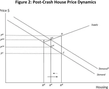
Figure 2 presents the market equilibrium E, boom B, and post-crash C price dynamics in
the owner-occupied housing market. I assume that pre-boom prices in 2001 were based solely on
the underlying fundamentals of supply and demand. Thus, prices were in equilibrium in Figure 2
at 𝑃𝐸. Liu et al. (2014) show that house price increases from 2004-2006 were not justified by
fundamentals, and that in response speculative developers expanded the housing stock (from 𝐻𝐸
to 𝐻𝐵). The housing bubble burst in 2007 and the anticipated demand never materialized, so
prices must eventually fall to 𝑃𝐶 on the demand curve for the market to clear (Glaeser et al. 2008; Liu et al. 2014). The downward price correction is magnified if lending standards are
tightened or unemployment increases as a result of the bubble bursting (Haughwout et al. 2012).
In Figure 2, I also present a model of post-crash housing market dynamics. Unlike
previous research I do not assume that the supply of housing is fixed. Thus, the shift from 𝐻𝐵
back towards 𝐻𝐸 represents the reduction in available owner-occupied housing stock. The cost to
convert a property from owner-occupied to a rental is negligible, so institutional investors can
easily convert a house to a rental property, and vice-versa when the market rebounds. However,
when institutional investors purchase and convert houses to rentals they pay cash and no longer
benefit from owner-occupied housing’s preferential tax treatment. As such, institutional investors
pay lower prices relative to homeowners for owner-occupied housing. The difference in price
16
[Insert Figure 2]
As institutional investors purchase owner-occupied houses and convert them to rental
housing they reduce the available owner-occupied housing stock and push the market back
towards equilibrium. In my model, institutional investors target owner-occupied housing with the
highest anticipated yields based on (1) expectations of mean reversion in prices and (2) rental
income.24 In doing so, institutional investors impose a disciplining effect by reducing the
available housing stock. As the housing stock shifts inward to 𝐻#, prices move up the demand
curve from C towards 𝐶#, thereby reducing the relative price divergence.25
Thus, the model
supports institutional investors’ expectations of mean reverting prices.
If the market’s population continues to grow and the single-family housing market begins
to recover, the model predicts that demand will gradually increase. As demand increases, prices
will move up the supply curve from 𝐶# to 𝐸#. As prices increase and demand grows, some
institutional investors will convert their properties back to owner-occupied housing by listing
them for sale instead of renting them out. As institutional investors reintroduce the converted
houses back to the owner-occupied housing market they gradually shift the available housing
stock back towards 𝐻𝐵. As institutional investors convert and sell their rental properties to
owner-occupiers prices will move up the demand curve from 𝐸# to B.
6. Data
The analysis in this paper focuses on single-family detached homes in the Atlanta, GA
metropolitan area.26 Atlanta is the ideal setting for this study as it attracted considerable
institutional investment after the real estate crash. In their examination of large “buy-to-rent”
investors, Mills, Molloy and Zarutskie (2015) find that Atlanta had the second highest
buy-to-rent market share in 2012 – only Phoenix, AZ (6.5%) had a higher market share than Atlanta’s
24
I examine institutional investors’ expected returns in Section 6.
25
If lending standards are tightened or unemployment increases, the demand for housing will decrease and the demand curve will shift inwards resulting in lower prices (Haughwout et al. 2012). Regardless, owner-occupied houses redeployed as rental housing will reduce the available owner-occupied housing stock and prices will increase up the ‘reduced’ demand curve.
26
17
6.4%. In 2013, Atlanta (11.6%) had the second highest market share again - Winston-Salem, NC
(12.2%) had the highest market share. In 2014, Atlanta (5.0%) had the fourth highest buy-to-rent
market share - only Charlotte, NC (6.6%), Jacksonville, FL (6.6%), and Memphis, TN (5.1%)
outpaced Atlanta (Mills et. al 2015).27
Atlanta’s housing market is also very similar to the United States market as a whole. As
displayed in Table 2, 36.5% of occupied housing units were rentals in both Atlanta and the
United States in 2013. In addition, prior to the real estate crash single-family detached housing’s
market share in Atlanta and the United States were nearly identical (25.4% in Atlanta versus
25.9% in the United States in 2007). In 2013, single-family detached rental properties accounted
for 31.7% of the Atlanta rental market after experiencing a 25.2% increase in the number of
rental units between 2007 and 2013. Single-family detached rental housing also grew across the
United States, albeit at a slower pace of 11.2% over the same time period, accounting for 28.8%
of the rental market in 2013.
[Insert Table 2]
The data for this study comes from several sources. The first two sources are datasets
compiled by CoreLogic. The first CoreLogic dataset contains county tax assessor records. The
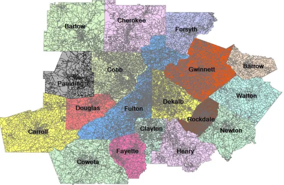
tax assessor dataset includes parcel level information for every property in the eighteen counties
that comprise the Atlanta, Georgia metropolitan market.28 The parcel file specifies whether there
is a structure built on the property and, if so, the type of structure (single-family detached,
multi-family, commercial, etc.). The parcel file also includes detailed information about the physical
characteristics of the structure, such as the square feet of living area, number of bedrooms,
number of bathrooms, and its lot size.
The second CoreLogic dataset includes every property transaction recorded in the
eighteen counties from January 1st, 2000 through December 31st, 2014. I use several fields in the
dataset to identify and isolate single-family detached sales transactions. After applying several
27
Atlanta was the clear leader in terms of institutional investor purchase volume. Mills et al. (2015) estimate that institutional investors purchased approximately 17,660 single-family homes in metro-Atlanta from 2012-2014. Of the other markets listed – institutional investment volume was second highest in Tampa, FL where they purchased approximately 7,498 single-family homes from 2012-2014 (*Note: only the top 10 markets are listed for each year so it is possible that a market that was only listed once or twice had a higher volume than Tampa, FL).
28
18
filters that remove (i) single-family attached, multi-family, and commercial sales transactions,
(ii) interfamily transactions, and (iii) non-purchase transactions, the final dataset includes
approximately 1.25 million sales transactions. The data is well suited for the issues I address in
this paper as it contains detailed information about the parties involved in the transaction (i.e.
buyer and seller), terms of the transaction, and the type of deed conveyed. Thus, I can determine
whether an owner-occupier or investor purchased the property, it was part of a portfolio sale, or
it was a foreclosure, REO, or short sale.
The third data source I utilize was provided by the Georgia Multiple Listing Service
(GAMLS). The GAMLS dataset includes houses that were listed for sale or rent in the eighteen
counties in and around Atlanta, GA. The GAMLS sales data is available between 2000 and 2014
and the rental data is available between 2003 and 2014. The data collected from the GAMLS
includes detailed property characteristics (bedrooms, baths, etc.), listing information (list date,
sale date, etc.), and sale conditions (foreclosure, REO, etc.). As noted by Levitt and Syverson
(2008), MLS data is manually entered by real estate agents and is prone to error. Thus, I augment
and validate the MLS records with the CoreLogic tax assessor and sales transaction data.
6.1 Repeat Sales House Price Index
I create a quarterly repeat sales housing price index using the CoreLogic sales transaction
data that includes all single-family detached houses that were listed and sold at least twice during
the sample period of 2000 to 2014. The initial dataset contains 1,255,075 sales transactions, over
30% of which are attributable to houses that only sold once during the sample period. After
creating matched pairs, I remove records whose sales transactions occurred within six months of
each other. The final repeat sales sample includes 420,809 records. Following Case and Shiller
(1989) I estimate the index as follows:
Log(𝑃𝑖𝑡
𝑃𝑖𝑓) =∑ 𝛽𝑞 𝑞 𝐷𝑖𝑞+ 𝜀𝑖𝑡𝑓, q = 1, 2, … , Q (13)
where 𝐷𝑖𝑞 = {
1, if 𝑞 = 𝑡 −1, if 𝑞 = 𝑓 0, otherwise
𝑃𝑖𝑓 is the price of property i at the time of the first sale f
19
𝛽𝑞 is the estimated coefficient for quarter q
Q is the number of quarters in the study period
𝜀𝑖𝑡𝑓 is the error term
I report exponentiated values that are scaled to 100 in relation to the first quarter of 2001. Figure
3 presents the results for Equation 13 in the form of a repeat sales index. House prices in Atlanta
were relatively stable through the early to mid-2000s, increasing an average of 5.8% per year
from 2000 to 2006. Although Atlanta’s prices did not increase as much as other cities during its
boom period, its bust period was equally dramatic. House prices dropped by almost 50% during
the real estate crisis and remained at levels below those experienced in 2001 until the second
quarter of 2014.
[Insert Figure 3]
Single-family detached sales volume mirrored the growth of house prices as displayed in
Figure 4. The total volume of sales in the Atlanta metro area rose steadily from 2000 through the
second quarter of 2006, peaking at 32,831 quarterly sales transactions. Sales volume dropped
dramatically during the real estate crash as the percent of distressed sales rose rapidly, reaching
as high as 74.3% in the fourth quarter of 2010. Both home prices and sales volume increased
after 2012 and were approaching their pre-boom levels in the final quarter of 2014.
[Insert Figure 4]
6.2 Classification of Sales Transactions
Much of the analysis going forward relies on the correct identification and classification
of owner-occupiers and investors. As such, I meticulously identify and assign each transaction as
follows. To identify owner-occupiers I rely on a field provided in the CoreLogic dataset. I also
perform a validation using the legal mailing address of the properties that were flagged by
CoreLogic as occupied (where available). The validation checks whether an
20
additional properties in the dataset.29 If so, I assume those properties are not owner-occupied. If
the owner-occupier’s legal mailing address does not match any of the property addresses I
assume that the first single-family house purchased by the owner-occupier is their primary
residence and the remaining properties are investments.
All single-family detached housing transactions not attributed to owner-occupiers are
considered investor activity. I segment the investor transactions into two categories using an
indicator variable available in the CoreLogic dataset. The indicator variable identifies all
transactions in which the buyer is a corporate entity. If the indicator variable is 0, the transaction
is assigned to an individual investor. If the indicator variable is 1, I further segment the corporate
entity transactions into one of four investor subcategories: government/non-profit, financial
institution, institutional investor, or corporate investor. Government and non-profit transactions
include all purchases by government entities, such as local city and county governments, as well
as purchases by non-profit groups, such as Habitat for Humanity. Financial institution
transactions include all purchases by credit unions, securitized mortgage trusts, and banks.
To identify institutional investors I take a more granular approach as they are the primary
group of interest in this study. I classify a purchaser as an institutional investor if they (i) entered
the Atlanta housing market after the real estate crash, (ii) raised equity to invest in single-family
detached housing, (iii) purchased 200 or more single-family detached houses, and (iv) had a
publicly stated investment strategy of converting the houses they purchased to rentals.30 After
identifying eleven institutional investors, I associate all their transactions to their parent company
to ensure the classification is comprehensive and accurate.31 If the company is publicly traded, I
29
The legal mailing address is where the property’s owner receives property tax statements from the county. I cleanse the legal mailing addresses using an address verification system to remove typos and to ensure consistency in the dataset.
30
I investigated every company that purchased more than 25 single-family detached houses from 2007 to 2014. Several companies had more than 200 combined purchases, but were not classified as an institutional investor if their investment strategy differed. Opportunistic investors that purchased houses and sold them in a short period of time (i.e. flippers) are not included. In addition, local investors that already had a portfolio of single-family detached houses prior to the real estate crisis are not included in the classification. Thus, the classification identifies the institutional investors discussed in section 4.
31
21
identify and search the transaction records for every asset company name listed in their SEC
filings. If the company is private, I search their website for rental properties, look up the
properties’ owner in the CoreLogic dataset, and flag the asset company name as a known
subsidiary of the institutional investor (I also perform this task for institutional investors that are
public companies to ensure I capture all of their transactions). If a transaction is not assigned to
the government/non-profit, financial institution, or institutional investor classifications it is
placed in the corporate investor classification. A breakdown of sales transactions by buyer type
is available in Table 3, which I discuss in detail in the next section.
6.3 Atlanta’s Housing Stock and Investor Activity
Increasing house prices incentivized new development in the Atlanta market during the
early to mid-2000s as displayed in Table 3. The number of new single-family detached houses
introduced to the market remained relatively steady from 2000 to 2006, peaking at 48,245 new
units in 2006. The new houses represented an annual supply growth of approximately 4%, when
compared to Atlanta’s housing stock in 2000, and may explain why Atlanta’s house prices did
not rise as rapidly as other cities during the real estate boom. Development slowed during the
real estate crisis as prices crashed and the number of financial institution transactions nearly
doubled from 2005 to 2007. The number of individual and corporate investor transactions also
increased rapidly after the crash, almost doubling from an average of 6,321 purchases per year
(2000-2006) to 12,370 purchases per year (2012-2014).
[Insert Table 3]
6.3.1 Institutional Investment
Several market factors likely influenced institutional investors’ decision to enter the
single-family detached housing market including declining house prices, decreasing multi-family
vacancy rates, a large number of delinquent borrowers, the capital markets acceptance of
investments in residential Real Estate Investment Trusts (REITs), the prospect of bulk purchases,
and higher expected returns relative to apartment buildings. The repeat sales price index in
Figure 3 shows that house prices were falling in 2011 and bottomed out in the first quarter of
22
2012 – which corresponds with the entrance of institutional investors.32 Figure 5 shows that
demand for rentals was increasing as multi-family vacancy rates decreased from 13.1% in the
third quarter of 2009 down to 10.3% in the first quarter of 2012. In addition, there was very little
multi-family construction in the pipeline. From 2000 through 2008, approximately 74,000 new
multi-family units were started each quarter. In contrast, approximately 30,000 new multi-family
units were started each quarter from 2009 through 2011.
[Insert Figure 5]
Figure 1 shows that over 10% of homeowners were delinquent in 2011. The increased
demand for rentals was expected to continue because the delinquent homeowners would likely
become renters after they were foreclosed on. The delinquencies also meant that a large supply
of distressed single-family detached housing would be available for purchase in the near future.
The upcoming liquidation of distressed single-family detached housing combined with an
increasing demand for rentals and decreasing rental vacancies offered a unique opportunity for
large scale investment in and conversion of single-family detached housing.
Another potential draw for institutional investors was the capital market’s acceptance of
residential REITS. In January 2007, residential REITs accounted for $67 billion or 16.8% of the
equity REIT market capitalization (NAREIT 2007).33 Prior to the real estate crash, residential
REITs included apartment and manufactured home REITs. There were no single-family rental
REITs, but the market had a history of accepting and investing in new asset classes.34 The
growth and innovation of capital markets may have played a role in institutional investors’
entrance into the owner-occupied housing market in 2012.
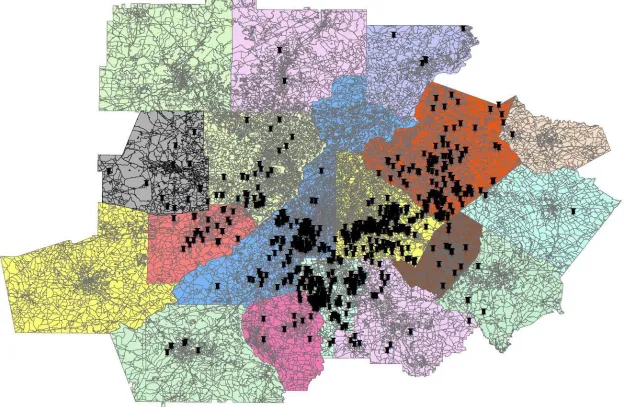
Table 3 highlights the entry of institutional investors into the Atlanta owner-occupied
housing market. Over a four year period, 2011 to 2014, institutional investors purchased 21,283
single-family detached houses in the metro Atlanta area. Although institutional investors
purchased a few properties in late 2011, it wasn’t until 2012 when they truly entered the Atlanta
market and accounted for over 5% of all the single-family detached housing transactions. In
32
The repeat sales price index in Figure 3 only includes sales transactions for metro-Atlanta. However, the start of Atlanta’s housing market recovery coincides with the start of the recovery nationwide
33
In December 2014, residential REITs accounted for $108 billion or 12.9% of the equity REIT market capitalization (NAREIT 2014).
34
23
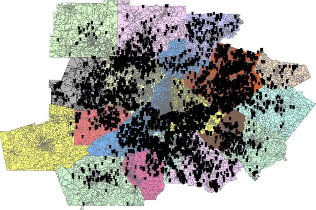
2013, institutional investment in Atlanta more than doubled, accounting for over 13% of all the
sales transactions in the market. Competition among investors and increasing prices curtailed
institutional investment in 2014, although they still accounted for over 8% of all single-family
detached sales transactions.
The publicly stated investment strategy of the institutional investors included in this study
is to purchase single-family detached homes and operate them as rentals.35 Prior to the real estate
crash, it was difficult for institutional investors to amass a portfolio of single-family detached
rental homes – as they usually were only available through one-off sales. Thus, the single-family
rental market remained fragmented in terms of both ownership and operation until after the real
estate crash when institutional investors had several avenues in which they could purchase and
build a portfolio of single-family detach rentals quickly including: individual sales, auctions,
short sales listed on the MLS, trustee sales (foreclosed and tax sale properties), bank-owned
houses listed on the MLS, bank-owned houses purchased directly from banks, and in some cases
bulk sales.36,37
Institutional investors purchased single-family detached houses in Atlanta through
several avenues as displayed in Table 4. Approximately 46.7% of their purchases were
foreclosures, 7.9% were REOs, 7.8% were short sales, and 5.5% were part of a bulk purchase.38
Of the remaining non-distressed transactions approximately 18.8% were purchased directly from
an owner-occupier, 12.7% were purchased from an investor who already converted the property
to a rental, and 0.6% were purchased from investors who owned and rented the house prior to
2007. The largest institutional investor in Atlanta was the Blackstone Group, through their
Invitation Homes subsidiary. The Blackstone Group accounted for over one-third of all
35
See, for example, the American Homes 4 Rent website - https://www.americanhomes4rent.com/ - which states that they are “focused on acquiring, renovating, leasing and operating attractive, single-family homes as rental properties.”
36
Citing a 1996 Property Owners and Managers Survey, Mills et al. (2015) state that three quarters of the single-family detached rental units were owned by individuals or partnerships that owned fewer than 10 units.
37
Auctions, short sales, trustee sales, and bank-owned sales were available prior to the real estate crash – but their volume paled in comparison to their post-crash volume (see Figure 4).
38
24
institutional purchases and was the primary bulk purchaser in Atlanta.39 Although bulk sales only
represented 5.5% of institutional investors’ single-family purchases in the Atlanta - the prospect
of bulk purchases may have drawn institutional investors into the market. In February 2012, the
Federal Housing Financing Authority (FHFA) and Fannie Mae announced a REO-to-Rental Pilot
Initiative to determine if bulk sales would generate private investment in single-family rental
housing.40
[Insert Table 4]
6.4 Institutional Investors’ Expected Return
The liquidation of distressed single-family housing may offer a unique investment
opportunity, but institutional investors are rational and will only enter the owner-occupied
market if it offers higher returns than apartment buildings in the rental market. In this section, I
compare institutional investors’ competing investment alternatives in rental housing (apartment
buildings) with owner-occupied housing (single-family detached houses).
6.4.1 Mean Reversion Expectations
To examine institutional investors’ mean reversion expectations I use the same dataset
described in Section 6.2 to create a repeat sales index by investor type. The results displayed in
Figure 6 show that institutional investors were able to identify and purchase single-family
detached houses that offered higher expected mean reverting returns relative to individual
investors and owner-occupiers. Institutional investors place a lower value on owner-occupied
housing because they must convert it to rental housing, so the higher expected mean reverting
returns are a product of, among other things, owner-occupied housing’s asset illiquidity and
preferential tax treatment.
[Insert Figure 6]
39
The overwhelming majority of Blackstone’s transactions that are flagged as bulk purchases can be attributed to one deal that they completed in April 2013 with Building and Land Technology’s single-family rental business.
40
Additional information on the REO-to-Rental Pilot Initiative is available on the FHFA website:
25
Figure 7 plots an annual repeat sales index that that has been stratified into twenty home
size segments based on each houses’ square feet of living area. The stratified home size segments
are a proxy for housing quality and that help identify the housing segments that institutional
investors targeted. I stratify the home size segments in ascending order, so the smaller the house
is, the lower the percentile it is segmented into (i.e. 0-5 percentile contains the smallest houses
and 95-100 percentile contains the largest houses). Although the boom period in Atlanta was
relatively mild compared to other cities, Figure 7 suggests that prices in two segments of
Atlanta’s single-family detached housing market, the 0-5 and 5-10 percentile, increased at a rate
much higher than the rest of the market. The same two segments also experienced the largest
decline during the crash.
[Insert Figure 7]
Next, I quantify and compare the mean reversion expectations by home size segment and
buyer type in Table 5. The top section of Table 5 is stratified into the same twenty home size
segments that correspond with Figure 7 – it details each home size segments’ size distribution,
number of properties purchased by institutional investors, and mean reversion expectations.
Although institutional investors were active in every home size segment, the majority (over 85%)
of their purchases fell in the 5-75 percentile range. The top right section of Table 5 provides the
price index levels by home size segment for the pre-boom index level (𝑃𝐸) in 2001, the pre-crash
price apex (𝑃𝐵) in 2006, the post-crash nadir (𝑃𝐶) in 2012, and the recovery price in (𝑃𝑅) in 2014. I also calculate each home size segment’s pre-crash price appreciation (𝑃𝐵 - 𝑃𝐸), post-crash price depreciation (𝑃𝐶 - 𝑃𝐵), and mean reversion expectations in 2012 (𝑃𝐸 - 𝑃𝐶) and 2014 (𝑃𝐸 - 𝑃𝑅). The last two columns of Table 5 clearly show that smaller houses offered higher expected mean reversion returns in both 2012 and 2014. The monotonic price declines explain
why institutional investors preferred smaller houses and were not as active in the 75-100
percentile home size segments.
[Insert Table 5]
In the bottom section of Table 5 I create price index levels by buyer type to compare
institutional, corporate, and individual investors. The price index levels correspond with the