Munich Personal RePEc Archive
Price Deviations of SP 500 Index
Options from the Black-Scholes Formula
Follow a Simple Pattern
Li, Minqiang
Gerogia Insititute of Technology
2008
Price Deviations of S&P 500 Index Options from the
Black-Scholes Formula Follow a Simple Pattern
Abstract
1. Introduction
It is well known (see, e.g., Rubinstein (1994)) that if one uses the Black-Scholes formula or the
binomial model with the same volatility to compute option values for different strike prices but the
same time to expiration, the computed option prices deviate from quoted prices. Equivalently, for
a fixed time to expiration the implied volatility function obtained by inverting the Black-Scholes formula or binomial model is a non-constant function of the strike price. Depending on the shape,
this relation between the option strike price and implied volatility is known as the volatility smile
or skew. The smile or skew is by now viewed as a basic feature of most option markets, and its
presence is apparent in even the most cursory examinations of option implied volatilities. Similarly,
it is well known that option implied volatilities differ with the time remaining to expiration. Both
this phenomenon and the smile or skew are captured by the implied volatility surface, which is the
function mapping the strike price and time to expiration to implied volatility.
This paper presents a new approach for describing the differences between actual option prices
and their Black-Scholes values (computed with the same volatility for different strikes), which we
term the price deviation function, as well as the associated implied volatility function. It also presents new empirical results about the dynamic behavior of the deviations of actual S&P 500
index (SPX) option prices from their Black-Scholes values and the associated implied volatility
function. While both the price deviation and implied volatility functions vary randomly over time,
we find that during the period 1996–2002 SPX option prices follow a stable pattern that allows the
price deviation function to be well approximated by a simple function of the at-the-money-forward
“total volatility,” defined as the product of the at-the-money-forward volatility and the square root
of the time to expiration. Thus changes in the slope and curvature of the implied volatility function
are almost completely explained by changes in the at-the-money-forward total volatility.
A large literature addresses the volatility skew, much of it consisting of papers proposing
mod-els that produce volatility skews, smiles, or both. The simplest such modmod-els are the deterministic volatility function models in which the stock price follows a diffusion process with a diffusion
coeffi-cient or instantaneous volatility rate given by a deterministic function of the stock price and time.1
Other approaches to capturing the smile or skew include superimposing jumps on the price process
of the underlying asset, allowing for stochastic volatility by introducing an additional process to
1
describe the movement of the instantaneous volatility, or both.2 Recently, there is also a growing
literature on using the L`evy process to model the price process, thus allowing for more flexibility
in the behavior of the jumps.3 However, evidence on the empirical performance of these models is mixed. Using data on the prices of SPX options, Dumas, Fleming, and Whaley (1998) perform
out-of-sample empirical tests of the deterministic volatility functions and find that they are
outper-formed by anad hocimplementation of the Black-Scholes model that smooths the implied volatility
function across strike prices and time to expiration and uses the estimated implied volatilities to
calculate option prices one week later. Brandt and Wu (2002) reach similar conclusions using data
on FT-SE 100 index options. Bakshi, Cao, and Chen (1997) and Bates (1998) compare the pricing
and hedging errors of various models and obtain results generally consistent with the idea that a
model with both discontinuous “jumps” and stochastic volatility performs better than the
Black-Scholes model using the same volatility for different strike prices. Jackwerth and Rubinstein (2001)
run an extensive horse race and find that, although the Black-Scholes model is outperformed by both deterministic and stochastic volatility models, the variability of the pricing errors is so large
that it is not possible to rank the competing models. Moreover, it is difficult to reconcile the slope
(and changes in the slope) of the implied volatility function with the parameters of the empirical
distribution of returns and reasonable estimates of investors’ risk aversion (Bakshi, Cao, and Chen
(1997), Bates (2000), Jackwerth (2000), and Bondarenko (2001)).
A common feature of the deterministic volatility function, stochastic volatility/jump-diffusion,
and L`evy process approaches is that they attempt to find a stochastic process that generates a
risk-neutral density consistent with the implied volatility function. An alternative approach to explain
the skew is that option prices may differ from their no-arbitrage values due to the costs and difficulty of executing the dynamic trading strategies that appear in the derivations of options’ no-arbitrage
values.4 Despite the lack of consensus about the cause or causes of the skew, certain stylized facts
2
Examples of these approaches include the jump-diffusion models of Merton (1976) and Bates (1991), the stochastic volatility models of Hull and White (1987), Scott (1987), Wiggins (1987), Melino and Turnbull (1990, 1995), Stein and Stein (1991), and Heston (1993a), the combined stochastic volatility jump-diffusion models of Bates (1996) and Bakshi, Cao, and Chen (1997), and the general affine model analyzed in Duffie, Pan, and Singleton (2000).
3
Examples of this approach include the variance-gamma model of Madan and Seneta (1990), Madan and Milne (1991), Madan, Carr, and Chang (1998), the log-gamma model of Heston (1993b), the hyperbolic model of Eberlein, Keller, and Prause (1998), theα-stable models of Janicki, Popova, Ritchken, and Woyczynski (1997), Popova and Ritchken (1998), and Hurst, Platen, and Rachev (1999), the CGMY model of Carr, Geman, Madan, and Yor (2002), and the log stable models of McCulloch (1987, 1996), and Carr and Wu (2003a). Other studies on applications of L`evy processes include Geman, Madan, and Yor (2001), Carr and Wu (2003b), and Carr and Wu (2004).
4
about it are known. First, for index options the implied volatility is generally a decreasing function
of the strike price, i.e. the implied volatility function is negatively sloped. Second, for individual
equity options the implied volatility function is generally convex and more symmetric or “smile-shaped” than the implied volatility function for index options, and it is less negatively sloped.5
Third, both the level and slope of the implied volatility function for index options appear to change
randomly over time.6
This paper presents new stylized facts about the volatility skew. We begin by expanding the
deviations of actual prices from Black-Scholes values using parabolic cylinder functions. It suffices to
use only two such functions, corresponding to the odd and even components of the price deviations.
For a large neighborhood of the forward price of the underlying asset, these two components can
be interpreted as the slope and curvature of the price deviation function, and can be mapped
to the slope and curvature of the implied volatility function. Using data on SPX options for the
period 1996–2002, the coefficients of both the odd and even components can be well fit as quadratic functions of the at-the-money-forward total volatility. That is, changes in the volatility skew are
almost completely explained by changes in the at-the-money-forward total volatility. This relation
is stable during the period 1996–2002. In particular, the term structure of at-the-money-forward
volatilities determines the entire volatility surface. This finding of stability in the price deviation
and implied volatility functions stands in marked contrast to the view of a large fraction of the
literature. One difference is that most previous work has not focused on the slope and curvature of
the price deviation function. Perhaps more importantly, the slope and curvature of both the price
deviation function and the implied volatility function depend upon the total volatilityσF√τ, and
previous authors have not focused on this quantity.
Stability in the volatility skew implies corresponding stability in at least some features of the risk-neutral density. As shown by Breeden and Litzenberger (1978), the risk-neutral density can
be obtained by differentiating the value of a European call or put option with respect to the strike
price (and adjusting for the discount factor). Carrying out this computation using the fitted option
index options being used by a different clientele than their at-the-money counterparts. More recently, Gˆarleneau, Pedersen, and Poteshman (2006) describe a model in which limits to arbitrage cause option prices to deviate from their no-arbitrage values, and present empirical evidence consistent with that model.
5
The implied volatility function for the index options has not always been negatively sloped. Rubinstein (1994) reports that this phenomenon appears to date from the October 1987 stock market crash. Whaley (1986) and Sheikh (1991) document changes in the implied volatility function of index options during the period 1983–1985.
6
prices, we find that the implied risk-neutral density of index returns is bimodal. This finding has
implications for models with stochastic volatility or jump components, as it provides a stylized fact
that proposed models must capture and rules out models that cannot produce this property. The choice of parabolic cylinder functions also has nice consequences for the implied distribution, as it,
for example, integrates to one exactly and preserves put-call parity. The parametric form of the
distribution should also be useful to researchers who want to introduce skewness and kurtosis to
the return distribution. More generally, description of the deviations of actual option prices from
Black-Scholes values in terms of parabolic cylinder functions is likely to be useful for empirical
analysis because it provides a low-dimensional (i.e., small number of parameters) description of the
price deviation and implied volatility functions.
In related work (Li and Pearson 2006), they find that our skew model is useful in predicting
future volatilities. Specifically, they update the “horse race” among competing models originally
carried out by Jackwerth and Rubinstein (2001) using more recent option data set and more recent models. In agreement with Jackwerth and Rubinstein (2001), they find that trader rules dominate
mathematically more sophisticated models in predicting option prices. However, the simple pattern
in the implied volatility skew can be used to further improve the performances of the trader rules.
Perhaps surprisingly, the naive Black-Scholes model beats all mathematically more sophisticated
models after adjusting the skew shapes using the simple pattern.
The paper is organized as follows. Section 2 describes the deviations of actual option prices
from Black-Scholes values and presents the series expansion. Using this approach, Section 3 shows
that during the period 1996–2002 the deviations of actual prices from Black-Scholes values are well
described by a stable function of the at-the-money-forward total volatility. Section 4 connects the price deviation function to the implied volatility function, and shows that the implied volatility
surface also can be modeled as a function of the at-the-money-forward volatility. Then, Section 5
works out the implications for the implied risk-neutral density. Finally, Section 6 shows that the
simple function provides good conditional predictions of option prices. Section 7 briefly concludes.
2. Deviations of actual option prices from Black-Scholes values and
the series expansion
We begin by modeling deviations of actual option prices (closing bid-ask midpoints) from
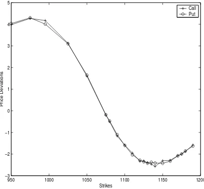
Black-Scholes values computed using at-the-money-forward volatilities. Figure 1 illustrates the deviations
observed at the close of trading on April 26, 2002 for the SPX options expiring in June 2002 as
a function of their strike prices. The Black-Scholes values are computed using the
forward price of the index. Because none of the traded options had strike prices exactly equal
to the forward price, the at-the-money-forward volatility is interpolated using cubic splines from
the implied volatilities of the straddles with strike prices surrounding the forward price, which on this day is estimated to be F = $1,072.49. Due to put-call parity the deviations for the puts are
essentially identical to those for the calls, and the deviations are zero at the strike price equal to
the forward price. As is known to be typical for the SPX options, for low strike prices the actual
prices exceed the Black-Scholes values, while for high strike prices the actual option prices are less
than the Black-Scholes values. One can see in Figure 1 that the deviations can be greater than $4
(at strike X = $975) and less than −$2 (near X = $1,150). For comparison, the bid-ask spreads
of both puts and calls at both of these strikes were $2. By simple model-independent arguments,
we expect that the price deviations should approach zero as the strike prices approach infinity or
zero, or equivalently as lnX approaches ±∞. Of course, options with strike prices of infinity and
zero are not traded, but the curves plotted in Figure 1 are consistent with this prediction.
Although the prices are the data directly observed from the market, many researchers and
practitioners focus on implied volatilities, and the implied volatility function is a widely used
rep-resentation of option prices. While working with implied volatilities is equivalent to working with
prices, working with prices overcomes several problems with implied volatilities. First, for
away-from-the-money options Black-Scholes option values are insensitive to changes in volatility. As a
result, small changes in option prices lead to large changes in implied volatilities, suggesting that
implied volatilities of away-from-the-money options may not be reliable and that any fitting
pro-cedure should place less weight on the implied volatilities of such options. Working in terms of
option prices is a natural way to accomplish this “deweighting” of away-from-the-money implied
volatilities. Second, dimensional analysis argues against separating the volatility σ and time to expirationτ from the combinationσ2τ that enters the Black-Scholes formula. It is not appropriate
to treat implied volatilities for different times to expiration on equal footing. Finally, although
there are some theoretical arguments (e.g., Hodges 1996, Gatheral 1999) restricting the asymptotic
behavior of the implied volatility as the strikeX approaches zero and infinity, such restrictions
usu-ally take the form of inequalities for the derivatives of implied volatility with respect to moneyness.
Because there are usually few away-from-the-money options available, it is difficult to calculate
these derivatives reliably, and these inequalities are awkward to implement. On the other hand,
it is much more natural and convenient to restrict the asymptotic behavior of option prices. For
these reasons we work with the deviations of actual option prices from Black-Scholes values.7
7
Besides overcoming the shortcomings of using implied volatilities, there are several advantages
of studying the price deviations directly. First, once we have fit the price deviations we can easily
use Taylor series expansion to obtain an estimated implied volatility function. In addition, the implied risk-neutral density can be easily obtained by differentiating the fitted prices. Further,
although our procedure does not guarantee the absence of convexity violations, it turns out that
such violations are minor and occur only at strike prices that are well away from the forward price.
2.1. Series expansion of the price deviations
The Black-Scholes formulas give the values of call and put options CBS and PBS as
CBS =F e−rτ
µ
N(d1)− X FN(d2)
, and PBS =F e−rτ
µ
−N(−d1) +
X
FN(−d2) 
, (1)
whereS is the current stock price or index value, ris the interest rate, δ is the dividend yield,σ is
the volatility, τ is the time to expiration,X is the strike price,F =Sexp((r−δ)τ) is the forward
price, and d1 andd2 are given by
d1=
ln(F/X) σ√τ +
1 2σ
√
τ , and d2=
ln(F/X) σ√τ −
1 2σ
√
τ . (2)
We callσ√τ the total volatility.
To compute the price deviations, we need to pick a volatility to use in the Black-Scholes formula.
We choose σF(t, τ), the at-the-money-forward volatility of an option with time to expiration τ at
calender date t.8 We make this choice because options with strikes close to the forward price are
usually actively traded with relatively small bid-ask spreads so thatσF can be computed accurately.
In addition, usually the forward price lies in the middle of the available strike prices because options
with strikes close to the new index level are introduced for trading as the index level changes. Thus
σF is obtained by interpolation (which is more reliable) rather than extrapolation.
necessary to satisfy the constraint. A further difficulty is that theoretical arguments do not restrict the tail behavior of the implied risk-neutral density. Thus, this approach provides little guidance in valuing options with strikes outside the range of strike prices for which implied volatilities are observed.
8
We measure the relative moneyness of an option using the quantity
d(t, τ, X) = ln(F(t, τ)/X) σF(t, τ)√τ
, (3)
which we call the total-volatility-adjusted moneyness or often simply moneyness. For example, a value of d = 2 roughly means that the option is two standard deviations in (for a call) or out
(for a put) of the money. For brevity, we often suppress the arguments in d(t, τ, X) and simply
write d, and similarly for F(t, τ) andσF(t, τ). Let YA(d) denote the actual market price of a call
or put option with moneynessd, letYBS(d, σF) denote the Black-Scholes value computed using the
at-the-money-forward volatility, and let
y=y(t, τ, X)≡ YA(d)−YBS(d, σF)
F (4)
denote the difference between the actual price and the Black-Scholes value, scaled by the forward
price. Scaling by the forward price is sensible because the Black-Scholes formula is homogenous of
degree one in the forward price. This scaling also makesy a dimensionless quantity.
We expand the deviations from Black-Scholes prices using parabolic cylinder function series. These functions are given by
Dn(z) = (−1)nez
2
/4 dn dzn
³
e−z2/2´
, n= 0,1,2, . . . . (5)
Expressions for the lowest order functions are:
D0(z) =e−z
2
/4 , D
1(z) =ze−z
2
/4 , (6)
D2(z) = (z2−1)e−z
2
/4 , D
3(z) = (z3−3z)e−z
2
/4 . (7)
A number of considerations lead us to this choice of parabolic cylinder functions. First, the functions Dn(z) (n = 0,1,2,· · ·) constitute a complete orthogonal function series on (−∞,+∞).
A function f(z) that: (i) has continuous first and second order derivatives; and (ii) goes to zero as
|z| → ∞ can be expanded usingDn(z) as (Wang and Guo (1989))
f(z) =
∞
X
n=0
anDn(z), where an=
1 n!√2π
Z ∞
−∞
f(z)Dn(z) dz. (8)
The parabolic cylinder functions can be used as a basis for deviations from Black-Scholes values
because it is reasonable to think that the deviations from Black-Scholes values satisfy condition (i)
z = a+blnX for some a and b. Thus, deviations from Black-Scholes values should permit an
expansion in terms of the parabolic cylinder functions. Further, the parabolic cylinder functions
are a natural choice of a function series because each functionDn(z) (n= 0,1,2, . . .) goes to zero
as|z| → ∞, suggesting that only a few terms will be needed. As shown below, this turns out to be
the case. Parabolic cylinder functions also facilitate the connections between price deviations and
implied volatility functions and between price deviations and the implied risk-neutral density, as
will be evident later on.
Temporarily fix a calender datetand a time to maturityτ. Expanding the scaled price
devia-tions in equation (6) in terms of the parabolic cylinder funcdevia-tions, we have
y ≡ YA(z)−YBS(z, σF)
F ≈
N−1
X
n=0
an(t, τ)Dn(z). (9)
where N is the number of functions we use and an, for n = 0,1, . . . , N −1, are the expansion
coefficients. This equation is for options with different strike prices for a fixed (t, τ) pair. Based
on the evidence in Section 3 below, we first drop the terms of third and higher order. Next, we choose the parameterzto bez=√2d, wheredis the total-volatility-adjusted moneyness defined in
equation (3) above. As pointed out above, choosingzto be a linear function of lnXautomatically
captures the asymptotic behavior of the price deviations. The factor√2 has the effect of making
the exponential factor exp(−z2/4) in the expressions for the parabolic cylinder functions equal to
exp(−d2/2), which is similar to a term that appears in the derivatives of the Black-Scholes formula.
As will be seen below, this is convenient when we relate the price deviations to implied volatilities.
An advantage of using dinstead of d1 is that when the strike price equals the forward price, the
quantities d, the left-hand side of (9), and D1(√2d) are zero. This constrains a0 = a2 on the
right-hand side of (9), enabling the use of one fewer expansion function.
After making these choices, the model of price deviations from Black-Scholes values is then
y ≡ YA(d)−YBS(d, σF)
F =a1Df1(
√
2d) +a2Df2(
√
2d), (10)
where
f
D1(z) =D1(z) = ze−z
2
/4, (11)
f
D2(z) =D0(z) +D2(z) = z2e−z
2
/4. (12)
functions of the at-the-money-forward total volatilityσF(τ)√τ:
a1 = (α1σF2(τ)τ +β1σF(τ)√τ) exp(−rτ), (13)
a2 = (α2σF2(τ)τ +β2σF(τ)√τ) exp(−rτ), (14)
where r = r(t, τ) is the risk-free interest rate. The details of the above fitting are explained
below. The coefficients α1, β1, α2, and β2 are stable over time in the sense that the same four
parameters fit the volatility skew for every calendar date and option expiration date over the period
January 1996–September 2002; the only parameter that varies with the calendar date and time to
expiration is the at-the-money-forward volatility σF(t, τ). Loosely, the slope and curvature of the
implied volatility function are determined by the at-the-money-forward total volatilityσF(t, τ)√τ.
Because on each calendar date we compute the at-the-money forward volatility for each option
expiration date, equation (10) is a model of the shape of the volatility skew or smile, and not a
model of the level of implied volatility. In Subsection 3.3.4 we combine equations (10) through (14)
and fit the implied volatility surface in a single step.
2.2. Interpretation of the parabolic cylinder functions
The two functions Df1 and Df2 that appear in the expansion (10) can be interpreted as the odd
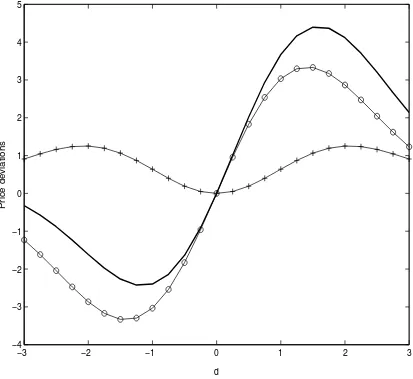
and even components of the deviations of actual option prices from Black-Scholes values. Figure 2
shows schematically how the two components sum to the price deviation function. The solid line shows the deviations of option prices from Black-Scholes values computed using the
at-the-money-forward volatility as a function of the volatility-adjusted moneyness d, while the lines with circles
and crosses show the odd and even components, respectively. Further, aroundd= 0, that is around
the forward price, the two components can be interpreted as the slope and curvature of the price
deviation function.
The first of the two components is clearly the more important. When we estimate the coefficients
a1 and a2 separately for each calendar date as described in the next section, the estimated values
of a1 are positive for the entire sample period, ranging from zero to about 0.05. The median value
ofa1 is 0.0082 while the mean is 0.0094. The estimated values ofa2 are both positive and negative,
mostly in the range of −0.005 to 0.005. The median of the absolute value of a2 is 0.00073 and the mean is 0.00085. When ln(F/X)/(σF√τ) = 1 (one standard deviation away from the money)
we have z = √2d =√2 and taking the median values of a1 and a2, the odd component is about
0.0082/(0.00073×2) = 5.62 times larger than the even component. For options that are close to
3. Fitting the price deviations
In addition to the choice of expansion functions, the model in equations (10)–(14) reflects three
further key choices. These are first, the decision to omit terms of third and higher order; second,
the decision to set a0 = a2; and third, the choice to specify the expansion coefficients a1 and a2
as functions of at-the-money-forward total volatility. In this section we first describe the data we used in this paper and then present the data analysis that motivated and supports these choices.
Subsection 3.4 below provides an empirical analysis of the fit of the model we used. In the next two
sections, we then connect our price deviation fitting with implied volatility fitting and the implied
risk-neutral density.
3.1. Data
The SPX option data used in this paper come from OptionMetrics LLC. The data include
end-of-day bid and ask quotes, implied volatilities, open interest, and daily trading volume for the
SPX (S&P 500 index) options traded on the Chicago Board Options Exchange from January 4, 1996 through September 13, 2002. The data also include daily index values and estimates of
dividend yields, as well as term structures of zero-coupon interest rates constructed from LIBOR
quotes and Eurodollar futures prices. The period from January 1996 until September 2002 includes
prices for options with 88 different expiration dates, including eight expiration dates that fall after
September 13, 2002.
We use the bid-ask average as our measure of the option price, and use all options that satisfy
the following criteria. First, we require that the option moneyness F/X satisfy 0.8 ≤F/X ≤1.2
and that the total-volatility-adjusted moneyness d= ln(F/X)/(σF√τ) satisfy−3≤d≤3, where
F is the forward price of the index,X is an option strike price,τ is the time to expiration, andσF
is at-the-money-forward volatility. Second, we use only options for which both bid and ask prices are strictly positive. Finally, we require that the time to expiration be greater than or equal to ten
business days. However, we keep all the long-term options with times to expiration up to 2 years.
We also require that for each strike price, there is a matching pair of put and call. These different
criteria overlap considerably. Imposing all criteria, we have 456,280 different option prices (228,140
calls and 228,140 puts).
These criteria are motivated by several considerations. First, they eliminate the least liquid
options. Second, they eliminate options for which the bid-ask average is unlikely to be a useful
approximation of the option value. Specifically, many of the away-from-the-money options are bid
at zero and offered at $0.5, with a bid-ask average equal to $0.25, independent of the time to
ten business days because our procedure requires prices for a range of different strikes, and for very
short times to expiration often only a few options satisfy the first two criteria.
3.2. Order of the expansion
Because parabolic cylinder functions form a basis for a function space, the price deviations can
be captured completely if sufficiently many functions are used. The question is then how many
functions are needed to capture the price deviations with a high degree of accuracy. There is
reason to think that the number of required expansion functions will be small, as Figure 2 suggests
that the two functionsDf1(z) andDf2(z) themselves explain a large fraction of the deviations from
Black-Scholes values.
To explore this issue, let us temporarily fix a calendar day t and time to expiration τ and
consider all the options with different strikes. Usingk to index the options with different strikes, we have
yk≡
YA(zk)−YBS(zk, σF)
F ≈
N−1
X
n=0
anDn(zk), (15)
where
zk=
√
2dk=
√
2 ln(F/Xk)
σF√τ
. (16)
Since we are fixing tand τ for now, we have omitted the dependence of t and τ in equation (15),
that is, we have writtenF forF(t, τ), σF forσF(t, τ),an foran(t, τ) and yk fory(t, τ, Xk), etc. If
we append an error term to the right-hand side, equation (15) can be thought of as an ordinary
least squares regression, with dependent variableyk and independent variablesDn(zk).
For each calendar day-expiration date pair, we estimate equation (15) using ordinary least
squares to obtain the expansion coefficientsan. We begin by looking at the squared errors. If there
areK available option series on day t, define the sum of squared errors in the usual way:
SSE=
K
X
k=1
à yk−
N−1
X
n=0 anDn(
√
2dk)
!2
. (17)
Defining the total sum of squares bySST =PKk=1(yk−y)¯ 2, where ¯y=PKk=1yk/K, the coefficient
of determinationR2 is given by R2 = 1−SSE/SST.
We illustrate the fit for different choices of N using the April 26, 2002 prices of the options
expiring in June 2002. Table 1 gives the sums of squared errors (SSE) and coefficients of
deter-mination R2 at the best fitting parameter values for N = 1,2, . . . ,7. Similar patterns of sums of
squared errors and R2’s with respect to N are found on other dates. Because the coefficients are
functionsN. However, there is no benefit to choosingN to be larger than six. First, doing this has
almost no impact on the sum of squared errors and the R2. Second, since we are not expanding
the entire price deviation function on each date (we typically have about 20 data points for each date), including more expansion functions may well result in over-fitting the data.
The discreteness of quoted option prices inherently limits the ability to obtain an exact fit with
a smooth function, suggesting it may be the case that the choice of N = 6 already overfits the
data, and that a choice as small asN = 3 might be reasonable. Further, the fact that the left-hand
side of equation (15) is zero when dk = 0, and the parabolic cylinder functions D0, D2, D4, . . . , are even functions places a constraint on the coefficients of these functions. In the case of N = 3
this constraint takes the form a0 ≈ a2, where the approximate equality comes from the fact that
the expansion does not provide an exact fit. Figure 3 illustrates that this approximate equality is
satisfied in the data when N = 3. In particular, Figure 3 shows the time series of the estimated
expansion coefficientsa0,a1, anda2for each day during the five month period prior to the expiration of the June 2002 options. The estimated coefficienta1 on the odd functionD1 declines steadily as
the time to expiration decreases from around 0.4 to zero, while the coefficients a0 and a2 on the
even functions D0 and D2 are approximately constant and equal to each other. In addition, with
this choice of N = 3 the R2’s are generally above 0.95 for each calendar day, declining below this
value only when the time to expiration becomes short. Table 1 also reports the fit for N = 3 but
with constraint a0 =a2 (column 2′) and we see that the R2 is almost as large as that for N = 3
without the constraint. Similar results are obtained for the other options with the same expiration
date and the options with different expiration dates.
For these reasons we choseN = 3 and constrain a0=a2, and thus use the expansion
yk≡
YA(dk)−YBS(dk, σF)
F =a1Df1(
√
2dk) +a2Df2(
√
2dk), (18)
where
f
D1(z) = D1(z) = ze−z
2
/4, (19)
f
D2(z) = D0(z) +D2(z) = z2e−z
2
/4. (20)
Figure 4 shows the time series of the expansion coefficients a1 and a2 obtained by estimating
equation (18). As expected, it is similar to Figure 3, with the only notable difference being that the time series of estimated expansion coefficients are smoother. Although (18) involves one less
3.3. Exploratory data analysis: Patterns in the expansion coefficients
The estimation of equations (15) and (18) by ordinary least squares discussed above is done
sepa-rately for each calendar day and expiration date, i.e. the procedure imposes no restriction on the
coefficients a1 and a2 across different days and expiration dates. Estimating the expansion (18)
separately for each calendar date-expiration date pair and imposing the constraint a0 =a2 results
in a total of 12,381 estimated coefficients a1 and a2. We seek stable relations that are satisfied by
the coefficientsa1 and a2.
We begin by using dimensional analysis as a rough guide, which has proven to be very useful in physics, engineering, and even pharmacology. The left-hand side of the expansion (18) consists
of price deviations divided by the forward price, and thus is dimensionless. Through the choice of
z = √2 ln(F/X)/(σF√τ) the quantities Df1 =ze−z
2
/4 and Df
2 =z2e−z
2
/4 also are dimensionless. Thus, the coefficients a1 and a2 must also be dimensionless, suggesting that they can only be
functions of dimensionless quantities. The available dimensionless quantities include the moneyness
F/X, the discount factor exp(−rτ) or equivalently rτ, the total dividends δτ, the total volatility
σF√τ, and d, d1 and d2. Among these, we can identify the following independent quantities: d, σF√τ,rτ andδτ. We disregardd, because the expansion should ensure that the dependence of the
price deviations on dis captured via the expansion functions, similar to the separation of variables
method in solving partial differential equations. Further, it seems unlikely that the dividend yield would vary enough to drive the variation in the coefficientsa1 and a2. Thus, dimensional analysis
suggests models of the form
an=fn(exp(−rτ), σF√τ), n= 1,2, (21)
where the fn’s are functions to be determined.
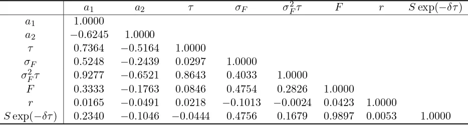
Table 2 confirms these tentative conclusions. It shows the correlations between the expansion
coefficients a1 and a2, the at-the-money-forward total variance σ2Fτ, the time remaining to
expira-tionτ, the volatilityσF, and some other variables. The correlations betweena1 and bothτ andσF
are high, with values of 0.7364 and 0.5248, respectively. However, the correlation betweena1 and
the total variance σF2τ is even higher, 0.9277. These correlations are larger than the correlations betweena1 and any of the other variables.9 While the magnitudes are smaller, a similar pattern is found in the correlations between a2 and the various variables. In particular, the correlation
be-tweena2 andσF2τ of−0.6521 is the largest of the correlations involvinga2. In the next subsection, we take a closer look at the odd and even components in turn.
9
Further, in untabulated results we find that the relatively large correlation betweenF anda1 is not stable across
3.3.1. The odd component
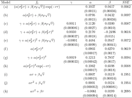
In the last section we preannounced that the model a1 = (α1σ2Fτ +β1σF√τ)e−rτ (equation (13))
in which a1 is a quadratic function of at-the-money-forward total volatility provides a good fit to
the expansion coefficient a1. Table 3 shows the coefficient estimates and sum of squared errors
(SSE) for a number of models for fitting a1. The total sum of squares SST of a1 for all seven
years is 0.4511. The first row of the table (model (a)) shows results for the quadratic model. The
sum of squared errors for this model is 0.0562. This implies that this model explains 88 percent
of the variation in a1. The second model (b) presents results for a version of the model that does not include the terme−rτ
. The coefficient estimates andSSE are similar, but the first model that
includes the term e−rτ
provides a slightly better fit. The next model (c) includes a constant term.
Unsurprisingly, the model with a constant term provides a better fit, in the sense that the SSE
is smaller. However, the estimated constant term is small, and not economically significant. The
next set of models (d)–(h) experiment with different functional forms of σF√τ and rτ, and find
that none dominates the quadratic model (a). Finally, the last three models (i)–(k) specify the
expansion coefficient a1 as a function of τ alone rather than σF√τ. Such models are problematic
a priorias they are not dimensionless, and the fit of these models turns out to be poor.
We next estimate the quadratic model (13) (i.e., model (a)) separately for each year. Figure 5
presents a three-dimensional view of the fit for the calendar year 2001 when the model is estimated using the option prices from year 2001. The parameter estimates are α= 0.0437 andβ = 0.0459.
In particular, Figure 5 plots the actual (dots) and fitted (stars) values of a1 for each calendar
date-expiration date pair during 2001 as a function of σ2
F and τ. For each actual value (each
dot), the fitted value is represented by the star immediately above or below it. Figure 6 presents
two-dimensional graphs obtained by projecting the data in Figure 5 onto the time to expiration,
volatility, and total variance σF2τ. Of each pair of panels, the left-hand panel shows the actual data and the right-hand panel shows the fitted values. This figure confirms that the quadratic
model (13) provides an excellent fit, and also confirms that the total volatility σF2τ explains the bulk of the variation in the coefficient a1. It is clear that the quadratic model (13) explains most
the variation ina1.
Figure 7 summarizes the fit of the quadratic model for the other years. In particular, it shows
the actual and fitted values of the coefficients a1 on the odd parabolic cylinder function Df1 as a
function of the total volatility σ2
Fτ separately for each of the five years 1996-2000 and the period
January 2001–September 2002. Each panel shows both the actual (gray dots) and fitted (black
dots) values. Volatilities were relatively low in 1996, and there was no SPX option with time to
expiration greater than one year in our sample. As a result, the data are concentrated toward the
all years except 1997 and 1998, and is reasonably good even for those years. In 1997 the quadratic
model still seems like a good choice, but there is considerable dispersion around the fitted values.
In 1998 there is a little less dispersion about the fitted values, and there seem to exist two patterns, with the fitted model roughly corresponding to the average of the two patterns. Also, volatilities
were high in this time period, and the relation is more steeply sloped than in other periods. The fit
is excellent for the remaining years, with similar shapes in 1999 and 2000 and a slightly less steeply
sloped relation in 2001 and 2002.
3.3.2. The even component
Table 2 shows that the correlation betweena2 and the at-the-money-forward total varianceσF2τ is
−0.6521, which is of greater magnitude than the correlation betweena2 and any other variable. In unreported graphical analysis we plotted a2 against the dimensionless quantitiesσF√τ and rτ as
well as several other variables for the entire sample. Consistent with the argument thata1 anda2
should be functions of only dimensionless quantities, we found no clear relation with the forward price, volatility, or interest rate.
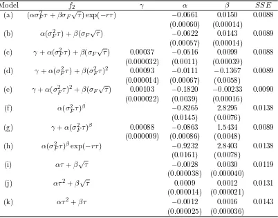
In the last section we preannounced that the model a2 = (α2σF2τ +β2σF√τ)e−rτ (equation
(14)) in which a2 is a quadratic function of at-the-money-forward total volatility provides a good
fit to the expansion coefficient a2. Table 4 shows the results of fitting this and alternative models
fora2. The table displays the coefficient estimates and sum of squared errors (SSE) for the same
set of models that are used to explaina1 above. As expected, sincea2 is much less variable thana1
and the time series of estimates have different properties, the coefficient estimate and SSE’s are
much different from those in Table 3. Nonetheless, as witha1 the quadratic model performs better
than all other models, although the differences from some of the other models are small.
Figure 8 shows the actual and fitted values of the coefficient a2 as a function of time to ex-piration τ, at-the-money-forward variance σ2
F, and at-the-money-forward total variance σF2τ for
calendar year 2001. Although botha1 anda2 are fit well by quadratic functions of the total
volatil-ity σF√τ, their patterns are quite different. Whilea1 seems to be monotone increasing in σF√τ,
a2 first increases and then decreases againstσF√τ and is nonnegative only for roughly the region
σF√τ < 0.06. As we will see later in Section 5, this has interesting implications for the second
central moment of the implied risk-neutral density. Of each pair of panels in Figure 8, the left-hand
panel shows the actual data and the right-hand panel shows the fitted values. This figure confirms
that the quadratic model (14) provides an excellent fit, and also confirms that the total volatility
Figure 9 summarizes the fit of the quadratic model fora2 for the other years. In particular, it
shows the actual and fitted values of the coefficientsa2 on the even parabolic cylinder function Df2
as a function of the total volatility σ2Fτ separately for each of the five years 1996-2000 and the period January 2001– September 2002. Each panel shows both the actual (gray dots) and fitted
(black dots) values. As with Figure 7, for 1996 the data are all toward the left-hand side because
there was no SPX option with time to expiration greater one year. We see that the fitted quadratic
model is generally similar in different years, though there is a fair amount of dispersion about the
fitted values in 1997 and 1998.
3.4. One-step estimation
The above exploratory data analysis used a two-step process. We first estimated the expansion coefficients a1 anda2 separately for each calendar date-expiration date pair, and then we searched
for models that captured the changes ina1 and a2. Having identified such a model, it is natural to
do the analysis in a single step. The one-step model is
y =α1X1+β1X2+α2X3+β2X4, (22)
where
y= YA(d)−YBS(d, σF)
F , (23)
and the right-hand side variables are
X1 =
√
2σ2Fτ dexp(−d2/2−rτ), (24) X2 =
√
2σF√τ dexp(−d2/2−rτ), (25)
X3 = 2σF2τ d2exp(−d2/2−rτ), (26)
X4 = 2σF√τ d2exp(−d2/2−rτ). (27)
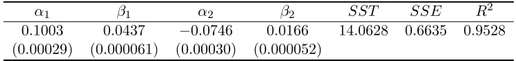
Notice that in equation (22) we are fitting all 456,280 call and put options simultaneously (228,140
(t, τ, X) triplets for both calls and puts). Estimating this model using the entire sample, we obtain
coefficient estimates α1 = 0.1003, β1 = 0.0437, α2 =−0.0746, andβ2 = 0.0166, and R2 = 0.9528,
as reported in Table 5. These estimates are similar to estimates for the quadratic models in Tables 3
and 4, where we have α1 = 0.1037, β1 = 0.0417, α2 = −0.0661 and β2 = 0.0150. These results
imply that the simple model with four parameters that are constant over time explains more than
95 percent of the deviations from Black-Scholes prices.
The above fit is excellent, in light of the fact that the discreteness of quoted prices inherently
exactly satisfied in the data. Notice that in our sample, we have both periods of rising index
levels and falling index levels. However, the changes in index levels do not seem to affect the
reported pattern although they affect the implied volatility levels. Also, we have options with time to expiration ranging from 10 days to 2 years. The fact that long-term and short-term
options both follow the same pattern is somewhat striking. In particular, this implies that the
relative expensiveness of out-of-the-money term options with respect to at-the-money
long-term options is not very different from the relative expensiveness for short-long-term options. Our results
also imply that SPX option traders have been pricing these options in a consistent manner for the
period 1996-2002.
4. Implied volatilities
The deviations of actual option prices from Black-Scholes values computed with the same volatility
for different strikes can be mapped into the implied volatility function through the inverse function
of the Scholes formula. This implies that the model (10)–(14) of deviations from
Black-Scholes values has an equivalent representation in terms of the implied volatility function. In
particular, the finding that the odd and even components of the price deviations are well fit by
simple functions of the at-the-money forward total volatility suggests that implied volatilities of
different strike prices can also be expressed in terms of the at-the-money forward total volatility.
In this section we use a Taylor expansion to find a simple approximation of this relation, and thus
connect our model of price deviations to a simple model of the implied volatility function. Our data set is the same one we used for the price deviation fitting. For each of the 12,381 calendar
date-expiration date (t, τ) pairs there is an implied volatility function computed from the straddles
for the different strike prices available. All together, there are 228,140 observations on the implied
volatility σ. Subtracting each of these implied volatilities from their corresponding
at-the-money-forward volatility for the same calendar and expiration dates, there are 228,140 observations of
implied volatility deviations ∆σ, defined as ∆σ=σ−σF.
4.1. A simple model of the implied volatility function
The model of price deviations (10)–(14) or equation (22) can be written as
YA(d)−YBS(d, σF)
Fexp(−rτ) exp(−d2/2) =
√
2(α1σ2Fτ +β1σF√τ)d+ 2(α2σF2τ +β2σF√τ)d2. (28)
Letting σ(t, τ, X) denote the implied volatility at calendar date t for time to expiration τ and
σF(t, τ), where as aboveσF(t, τ) is the at-the-money-forward volatility. Recognizing thatYA(d) =
YBS(σ) =YBS(σF + ∆σ), we can use a first-order Taylor expansion to obtain the approximation
YA−YBS(d, σF)
Fexp(−rτ) ≈ V∆σ
√
τ , (29)
whereV is the modified dimensionless vega defined by
V ≡ ∂(YBS(d, σ)/F∂(σ√exp(−rτ))
τ)
¯ ¯ ¯ ¯σ=σ
F
. (30)
Using the Black-Scholes formula, we see V = N′
(d1) ≈ N′(d) exp(−dσF√τ /2). Combining (28)
and (29) yields
V∆σ√τ
exp(−d2/2) =
√
2(α1σ2Fτ +β1σF√τ)d+ 2(α2σ2Fτ +β2σF√τ)d2. (31)
In our data, the mean value ofdis 0.24 and mean value ofσF is 0.21. Thus we can approximate
exp(dσF√τ /2) by 1 +dσF√τ /2. Using this, we get the following regression model
∆σ√τ =αdσF√τ +βd2σF√τ+γdσF2τ +δd2σF2τ. (32)
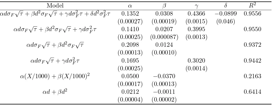
Table 6 presents the results of estimating the model (32) and some other models over the entire
sample period. The first set of results is for the model (32), which explains 95.56 percent of the
variation in ∆σ. The second set of results for the slightly simpler model
∆σ√τ =αdσF√τ +βd2σF√τ+γdσF2τ (33)
that omits the termd2σF2τ explains 95.50 percent of the variation in ∆σ. Due to the almost identical fits and the small magnitude of the term d2σ2Fτ in equation (32), we use the simpler model (33). The third and fourth sets of results are for two models obtained by restricting some parameters in
the full model to be zero, while the fifth and sixth sets are for two other models that are not based
on our expansion. The modelα(X/1000) +β(X/1000)2 (the fifth set of results) is the quadratic-fit
model of Shimko (1993). Although it is known that the Shimko model fits the volatility skew well
when estimated separately on each day, when estimated with the same parameters across calendar
days the Shimko model can only explain 22% of the volatility deviations. The last modelαd+βd2
is a quadratic fit in the volatility-adjusted relative moneyness d. While it performs much better
than the Shimko model its performance is still dominated by those of the first four models.
model in equation (33) for each calendar date-expiration date pair as a function ofd and dσF√τ
(only one out of 200 points are shown). The fit is perfect on the planes defined by d = 0 and
dσF√τ = 0 because on these planes the options are at-the-money forward, and hence their implied
volatilities do not deviate from the implied volatility of the at-the-money forward option from which
deviations are measured. Comparing the locations of the fitted values to the actual values, it is
clear that the quadratic model (33) explains almost all of the variation in the values of ∆σ.
Figure 10, while indicating a good fit, actually understates the quality of the fit because the
data density is not homogeneous on the graph. For example, there are many more options with
τ = 0.3 than options with τ = 2.0, and the bulk of the options with τ = 0.3 have fitting errors
that are very close to zero. However, these very small errors are hidden in the center of the figure
where the data density is high. The following numbers give us some sense of the quality of fit. Out
of all observations, 359 options (0.16%) have a fitting error larger than 0.05, 1,239 options (0.54%)
have a fitting error larger than 0.04, 3,615 options (1.58%) larger than 0.03, 10,548 options (4.62%) larger than 0.02, and 39,161 options (17.17%) larger than 0.01. In the other tail of the distribution,
14,3452 options (62.88%) have a fitting error smaller than 0.005, and 36.79% of the options have
an error less than 0.002. Also, the large errors concentrate in the years 1997 and 1998 (especially
in the months of August in both years), which is not surprising in light of Figure 7.
4.2. Implications of the implied volatility model
Our model captures the main features of the implied volatility surface and can be used to analyze
the slope and curvature of the skew. Fix a (t, τ) pair and hold the at-the-money-forward implied
volatility σF constant. Letting σX denote the implied volatility at strike price X for that (t, τ)
pair, we have
∂σX
∂lnX ¯ ¯ ¯
¯X=F =− α
√
τ −γσF. (34)
This equation says that there are two components to the slope of the skew. The first component,
−α/√τ, is a time-varying component that goes to zero as time to expiration increases to infinity. The second component, −γσF, is a volatility-level driven component. This component is present
even for τ =∞ and is proportional to the stochastic at-the-money-forward volatility level. Taken
together, the two components imply that the skew is negatively sloped, and becomes less so as the
time to expiration τ increases. Also, the skew tends to be more negatively sloped when volatility is high. Note that α and γ come from the odd component of the price deviations only, implying
that the odd component of the price deviation is directly responsible for the slope in the implied
It is also interesting to examine the curvature of the skew atX=F. From equation (33),
∂2σX
∂(lnX)2
¯ ¯ ¯ ¯
X=F
= 2β σFτ
. (35)
Sinceβcomes from the even component of the price deviations, this shows that the even component
in the price deviations is directly responsible for the curvature of the skew. The slope and curvature
of the skew can work together to produce a smile pattern. We see that the curvature is inversely
proportional to at-the-money-forward volatility level and time to expiration. As time to expiration
increases, the curvature decreases to zero.
The model (33) also provides an answer to the question of when we can expect to see a “smile”
in the implied volatility function. The implied volatility curve reaches its minimum at
d=−α+γσF
√τ
2β , (36)
which is about −3.5−10σF√τ for the parameter estimates we have. From the definition of d, we
have X=Fexp(−dσF√τ).If this turning point is low, then we are more likely to observe a smile
pattern in the traded options, which usually are roughly centered around the current index level.
Thus our model implies that we are likely to see a volatility smile more often whenσF√τ is small
(for example, in the relatively short-term options in year 1996) and whenr is small or the dividend
rate δ is large. We see that the volatility curve begin to increase again atX= 1.34F, when σF√τ
is about 0.07. This agrees with most stochastic volatility option pricing models, in which it is easier
to produce a smile when the instantaneous volatility and time to expiration are both small.
Some features of our results, however, are in contrast with one of the most common classes
of stochastic volatility models. Models in this class have no jumps, and specify an auxiliary in-stantaneous volatility process that is not explicitly dependent on the stock price levels, though the
Brownian motions driving the stock process and volatility process can be correlated. Specifically,
a typical model is specified as follows:
dS=rS dt+√V S dWS, (37)
dV =b(V) dt+a(V) dWV, (38)
where the two Brownian motions are correlated with coefficientρ(V) and the instantaneous variance processV is assumed to be mean-reverting. This class of models includes the now famous Heston
asymptotic behavior of the implied volatilities asτ →0 (p. 143) andτ → ∞(p. 187):
lim
τ→0
∂VX(τ)
∂lnX ¯ ¯ ¯ ¯
X=F
= ρ(VF(0))a(VF(0)) 2pVF(0)
, (39)
whereVX =σX2 is the square of implied volatility at strike price X, and
VX(τ)≈VF∞+
Aln(F/X)
τ +
Bln2(F/X) τ2 +O(τ
−3
) as τ → ∞, (40)
where A, B and V∞
F are some constants depending on the drift and diffusion functions of the
stochastic volatility process. That is to say, for very short-maturity options, the slope of the skew
tends to approach a constant while for long-maturity options, the skew tends to flatten to a common
asymptotic value regardless of the moneyness ln(F/X).
In our model, for short-maturity options,
∂VX
∂lnX ¯ ¯ ¯ ¯
X=F
=−2α
√
VF
√
τ −2γVF. (41)
In particular, the slope in our model atX=F approaches infinity at the speed of√τ. In comparing equation (41) with (39), one must be cautious because we have excluded options with maturities
less than 10 days and used a certain parametric form. However, in light of the fact that our model
explains over 95% of the variation in the implied volatilities it is hard to reconcile our empirical
results with the generic behavior of stochastic volatility models for short-term options.
Our results for long-maturity options are also at odds with the generic behavior of stochastic
volatility models. In our model,
VX(τ) =VF +
2α√VFτ + 2γVFτ
τ ln(F/X) +
(α+γ√VFτ)2+ 2β
τ ln
2(F/X) +O(ln3(F/X)). (42)
At a first glance, equations (40) and (42) seem similar because both express VX as a quadratic
function of ln(F/X). However, in our model VF does not approach a constant level but rather is
stochastic. Thus, there can be considerable variation in at-the-money-forward implied volatilities
even for long-maturity options. A second key difference is that in our model the slope of the
skew does not approach zero as τ → ∞, but rather approaches a stochastic slope −2γVF. A
third difference is the speed of convergence. In our model, if we hold VF constant, the speed
of convergence is 1/√τ. Interestingly, although it violates the long-maturity behavior of O(1/τ)
predicted by stochastic volatility models, this convergence agrees with the rule of thumb widely
used by practitioners that approximates the decay rate of the skew slope asτ−1/2
(see Lee 2002).10
10
5. Implied risk-neutral density
If the risk-free interest rate is constant, the value of a European call option can be written as
C=e−rτ
Z ∞
0
(ST −X)+f(ST)dST, (43)
where f(ST) is the marginal risk-neutral density of ST, the stock price at the expiration date
T. Prices of European put options can be characterized similarly. A standard result dating from
Breeden and Litzenberger (1978) is that the risk-neutral density is given by
f(ST) = erτ
∂2Y ∂X2
¯ ¯ ¯ ¯
X=ST
, (44)
where Y is the value of either a call or a put option. Since volatility is itself stochastic, this
implied density should be interpreted as the marginal density of some multi-dimensional risk-neutral distribution.
The price fitting model (10) can be written as
Y =YBS+ ∆Y ≡YBS+F(
√
2a1d+ 2a2d2)e−d
2
/2, (45)
where a1 = (α1σF2τ +β1σF√τ)e−rτ, a2 = (α2σ2Fτ +β2σF√τ)e−rτ, F = Stexp((r −δ)τ), d =
ln(F/X)/(σF√τ), and we have writtenrforr(t, τ),σF forσF(t, τ) etc. Differentiating, the implied
risk-neutral density fimp forST is given by
fimp=fBS+ ∆f, (46)
wherefBS is the lognormal density function
fBS =
1 q
2πσ2
Fτ ST
exp Ã
− ¡
logST −logSt−(r−δ−σ2F/2)τ¢2
2σ2
Fτ
!
, (47)
and
∆f = F e
−d¯2/2
erτ ST2σF√τ
(λ0+λ1d¯+λ2d¯2+λ3d¯3+λ4d¯4), (48)
where
¯
d= lnF−logST σF√τ
, λ0 =
√
2a1+ 4a2 σF√τ
, λ1 = 4a2−3
√
2a1 σF√τ
, (49)
λ2=−
√
2a1− 10a2 σF√τ
, λ3 =
√
2a1 σF√τ −
2a2, λ4 = 2a2 σF√τ
. (50)
Apart from the factore−rτ
,a1 and a2 are quadratic functions ofσF√τ, implying that theλ’s are
as well. Figure 11 plots the implied risk-neutral density computed using (46)–(50) above and the lognormal density on the same graph. The parameters used are σ = 0.15, τ = 0.2, S = 1,000,
r = 0.01, α1 = 0.1003, β1 = 0.0437, α2 = −0.0746, and β2 = 0.0166. These α’s and β’s are the
estimates from the one-step regression reported in Table 5.
A nice feature of this implied density given by (46)–(50) is that it is in closed form. Further,
other than the at-the-money-forward volatilities, it requires only four parameters, theα’s and β’s,
that describe the density for all strikes and times to expiration. Since one of the main results of this
paper is that these four parameters are very stable over time, one can use the parameters estimated
in this paper and treat them as constants. Thus, to use our parametric implied distribution, the
only input is the term structure of observed implied volatilitiesσF(t, τ).
The implied risk-neutral density has a number of other desirable properties. The first nice property is that our implied density is self-consistent, that is, if we let the strike price equal the
forward price, then the option price equals the Black-Scholes price evaluated at the
at-the-money-forward implied volatility:
Z ∞
0 e−rτ
(ST −F(t, τ))+fimp(ST) dST =CBS(σF(t, τ)). (51)
Similar results hold for the put options. Second, ∆f integrates to zero exactly, implying
Z ∞
0
fimp(ST) dST = 1, (52)
a necessary condition for fimp to be a sensible density. Third, the implied density gives the same
expected future stock price as the lognormal density, i.e.,
Z ∞
0
STfimp(ST)dST =F. (53)
The above equation says that our implied density satisfies the necessary condition to be a
and put-call parity since it implies
Z ∞
0 e−rτ
(ST −K)+fimp(ST)dST −
Z ∞
0 e−rτ
(K−ST)+fimp(ST)dST = (F −K)e−rτ. (54)
The above four equations can be easily derived, either by straightforward calculations or by repeated use of integration by parts. The implied density behaves so nicely because we have carefully chosen
σF as the base volatility and our model is, by construction, consistent with the prices of options;
and also because the parabolic cylinder functions used in our price model have good tail behavior,
that is, they go to zero exponentially as the moneyness dgoes to±∞.
It is interesting to examine the higher moments of our implied distribution. Using integration
by parts, it is easy to show that
Z ∞
0
(ST −F)2fimpdST =F2(eσ
2
Fτ −1) +F2 q
8πσ2
Fτ
³
2a2(1 +σF2τ)−
√
2a1σF√τ
´
e(r+σ2F/2)τ.
(55)
The first term on the right-hand side comes from the lognormal density, while the second term in-corporates the skew. With a bit of calculation it can be shown that the second central moment from
implied distribution will be equal to that from the lognormal distribution when eitherσF√τ = 0 or
σF√τ =.
√
2α2−β1+
q
(√2α2−β1)2+ 4√2β2α1 2α1
, (56)
which with our fitted parameters equals 0.142. If σF = 0.2, then this occurs with τ = 0.5009.
For a wide range of values of τ, the second central moments of the two distributions are close.
When τ is less than 0.5009 the second central moment from the implied distribution is larger than
the second central moment of the lognormal distribution. When τ is greater than 0.5, the second
central moment from the implied distribution is smaller than that from the lognormal distribution,
and the relative difference of the two goes to zero exponentially fast whenσF√τ goes to ∞. This
behavior comes from the fact thata2 is positive for smallσF√τ and becomes increasingly negative
asσF√τ increases.
Our implied risk-neutral density can also be viewed as a correction to the normality assumption
for lnST in the Black-Scholes formula. Our density approximation bears some similarity with the
often-used Gram-Charlier series expansion (see, e.g. Corrado and Su 1996, Backus, Foresi, and
Wu 2004) to correct for skewness and kurtosis. Both densities have a correction term involving a
fourth-order polynomial. However, a key difference is that our approach specifies the correction
aprpoxi-mation, one has to estimate or otherwise specify the skewness and kurtosis parametersµ3 and µ4
separately for each (t, τ) pair.
Finally, with suitable parameters the implied distribution can easily produce a volatility “smile.” In particular, the even component is responsible for the fat right tail in our risk-neutral density. It
is also responsible for the upward curvature that appears toward the right-hand side of the implied
volatility function shown in the lower panel, i.e. the fat right tail produces the volatility smile.
Although we do not pursue the issue here, the ability of the model to produce a volatility smile
suggests that it may be able to work well with individual equity options for which the smile is more
pronounced than it is in index options (although the American feature of the individual equity
options complicates matters).
The most straightforward use of the implied density would be to value European-style options
that are not actively traded, i.e. options with strike prices that are not actively traded, or digital
options. A more interesting aspect of the implied density is that we observe a second mode or peak in the density. A small and relatively “flat” second mode can be seen toward the left-hand side of
Figure 11. This second mode is produced by the even component, and its size depends both upon
the parameters α2,β2 of the even component and the level of the total base volatility σF√τ.
Figure 12 compares the lognormal and implied densities for a range of times to expiration,
namely 7, 31, 61, 91, 122, 182, 365 days and 2 years. The graphs in the various panels are
constructed usingσ = 0.25,S = 1,000, andr= 0.05, with theα’s andβ’s estimated from options
in our sample with times to expiration within a small window of the times to expiration indicated
on the panels. Except for the shortest maturity graph (the one labeled 7/365), the parameters are
estimated from options with times to expiration falling within an eight day window centered on
the time to expiration indicated on the panel. The shortest maturity graph is based on parameter estimates obtained from the options with times to expiration of between 10 and 15 days. We use an
eight day window to ensure that we have enough observations to calculate the local estimates for
α’s andβ’s reliably. It is interesting to see that on all the panels the implied densities are bimodal,
with the second mode gradually developing as time to expiration increases.
This finding of a bimodal risk-neutral density has implications for models with stochastic
volatil-ity and/or jump-diffusion processes, as it provides a stylized fact that proposed models must capture
and thus rules out models that cannot produce this property. A possible concern is that the
bi-modality is due to some artifact of the methodology of expanding price deviations in terms of
parabolic cylinder functions, and is not a robust feature of the data. One response is that the second peak is due to the even component, and Figure 2 illustrating how the odd and even
compo-nents sum to the price deviations makes clear that the even component is important in capturing
bimodality in the risk-neutral density using other approaches. Third, mathematically it is perfectly
possible for the risk-neutral distribution to be bimodal while the physical distribution is unimodal.
Bakshi, Kapadia and Madan (2003) shows how risk-neutral density of the return can have nonzero skewness while physical distribution is symmetric through exponential tilting which comes from the
Radon-Nikodym derivative. The same mechanism can also introduce bimodality in the risk-neutral
distribution.11
6. Conditional out-of-sample forecasting of the skew
The previous analyses show that the models of the skew provide better in-sample fits than a wide
range of alternatives. In this section we conduct a conditional out-of-sample forecasting exercise to verify that the proposed models perform better in this sense as well. This exercise is conditional
in that we do not predict the entire price or implied volatility function, but rather predict option
prices (i.e., the skew) conditional on the index value and the term structure of at-the-money-forward
implied volatilities. Specifically, for each calendar datet we start by estimating the parameters in
the selected models from a rolling window of past data. We then step ahead to a forecast date
t+ ∆t, and, given the index value and at-the-money-forward volatility on t+ ∆t, we use the
estimated parameters and the model to predict the price (or equivalently, volatility) deviations,
that is to predict the skew. Thus, this exercise only tests whether our models can correctly value
the away-from-the-money options, given the valuation of the at-the-money-forward options.
Interestingly, this exercise is similar to the way the models might be used in risk measurement, for example value-at-risk calculations. In some methods of computing value-at-risk one simulates
realizations of the underlying market factors that drive price changes, and then revalues the portfolio
of financial instruments for each realization of the market factors. If one takes the market factors
to be the underlying index value and the at-the-money-forward volatilities, then the exercise in this
section corresponds to this potential use of the models.
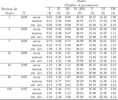
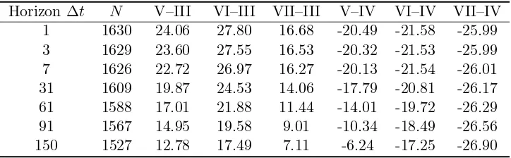
We compare a total of seven models. Models I and II are the models of price and volatility
deviations from Sections 3 and 4, respectively. Model III is a special case of Model II with one
fewer parameter. Then Models IV through VII are various plausible alternative models. For each
calendar date, we estimate the model parameters using data from the previous two months. We
11
Consider the following artificial example. Suppose the physical distribution of the future stock returnRis
f(R) =Aexp(−λR
2
)
1 +BR2 , where λ >0, B >0. (57)
This physical distribution is unimodal. Now with exponential tilting factor exp(−kR), if the parametersλ,kandB