wider use, because the implementation of FPGA architectures at the register transfer level is time consum-ing and error prone. Existconsum-ing software languages supported by high-level synthesis (HLS), although pro-viding a productivity improvement, are too general purpose to generate efficient hardware without the use of hardware-specific code optimizations. Such optimizations leak hardware details into the abstractions that software languages are there to provide, and they require knowledge of FPGAs to generate efficient hardware, such as by using language pragmas to partition data structures across memory blocks.
This article presents a thorough account of the Rathlin image processing language (RIPL), a high-level image processing domain-specific language for FPGAs. We motivate its design, based on higher-order algo-rithmic skeletons, with requirements from the image processing domain. RIPL’s skeletons suffice to elegantly describe image processing stencils, as well as recursive algorithms with nonlocal random access patterns. At its core, RIPL employs a dataflow intermediate representation. We give a formal account of the compilation scheme from RIPL skeletons to static and cyclostatic dataflow models to describe their data rates and static scheduling on FPGAs.
RIPL compares favorably to the Vivado HLS OpenCV library and C++ compiled with Vivado HLS. RIPL achieves between 54 and 191 frames per second (FPS) at 100MHz for four synthetic benchmarks, faster than HLS OpenCV in three cases. Two real-world algorithms are implemented in RIPL: visual saliency and mean shift segmentation. For the visual saliency algorithm, RIPL achieves 71 FPS compared to optimized C++ at 28 FPS. RIPL is also concise, being 5x shorter than C++ and 111x shorter than an equivalent direct dataflow implementation. For mean shift segmentation, RIPL achieves 7 FPS compared to optimized C++ on 64 CPU cores at 1.1, and RIPL is 10x shorter than the direct dataflow FPGA implementation.
CCS Concepts: •Computing methodologies→Image processing; •Computer systems organization →Data flow architectures; •Hardware→Reconfigurable logic and FPGAs; •Software and its en-gineering→Domain specific languages;
We acknowledge the support of the Engineering and Physical Research Council, grant references EP/K009931/1 (Pro-grammable Embedded Platforms for Remote and Compute Intensive Image Processing Applications), EP/N014758/1 (The Integration and Interaction of Multiple Mathematical Reasoning Processes), and EP/N028201/1 (Border Patrol: Improving Smart Device Security Through Type-Aware Systems Design).
Authors’ addresses: R. Stewart, K. Ducan, and G. Michaelson, Mathematical and Computer Sciences, Heriot-Watt Univer-sity, Edinburgh, UK, EH14 4AS; emails: {R.Stewart, krd1, G.Michaelson}@hw.ac.uk; P. Garcia and A. Wallace, Engineer-ing and Physical Sciences, Heriot-Watt University, Edinburgh, UK, EH14 4AS; emails: {P.Garcia, A.M.Wallace}@hw.ac. uk; D. Bhowmik, Department of Computing, Sheffield Hallam University, Sheffield, UK, S1 1WB; email: Deepayan. [email protected].
This work is licensed under a Creative Commons Attribution International 4.0 License
2018 Copyright is held by the owner/author(s). Publication rights licensed to ACM. ACM 1936-7406/2018/03-ART7 $15.00
Additional Key Words and Phrases: Domain specific languages, Parallel processing, Dataflow, FPGA, Hard-ware accelerators, Image processing, RIPL, Semantics, Cyclo static dataflow, High level synthesis, OpenCV ACM Reference format:
Robert Stewart, Kirsty Duncan, Greg Michaelson, Paulo Garcia, Deepayan Bhowmik, and Andrew Wallace. 2018. RIPL: A Parallel Image Processing Language for FPGAs.ACM Trans. Reconfigurable Technol. Syst.11, 1, Article 7 (March 2018), 24 pages.
https://doi.org/10.1145/3180481
1 INTRODUCTION
Video analytics has witnessed a major growth in applications including surveillance, vehicle auton-omy and driver assistance, marketing, entertainment, intelligent domiciles, and medical diagnosis. These domains need high performance, which can be achieved with parallel processing. Parallel image processing is most commonly performed on multicore CPUs and GPUs. This is because the data parallel nature of image processing algorithms maps well to multicore architectures, and because mature programming frameworks for them are widely adopted. Array-based image pro-cessing computations can be chunked into smaller single instruction, multiple data (SIMD) work items, then mapped across threads at each processor core and compiled to vectorized machine instructions at each core. The implementations of array/image processing languages for CPUs and GPUs (e.g., Chakravarty et al. (2011)) often store image data into memory close to processor cores, where the memories match complete images. Although compilers for these languages try to achieve good data locality, cache misses can cost idle clock cycles, which is critical because band-width between a processor and memory is often the most significant factor in determining overall performance (Wulf and McKee1995).
As the volume of image data collected from sensors grows, there is a strong need to process the data close to the sensor, to considerably reduce the amount of data to be transferred between sensors or to perform real-time processing, and to maximize the lifetime of nonpowered energy sources.
Hence, two factors make FPGAs more suitable than CPUs and GPUs for real-time image processing:
(1) Predictability. Real-time image processing performance must be predictable—that is, it must not fluctuate below a frames per second (FPS) threshold, because that may compro-mise algorithmic robustness. Cache misses on fixed CPU/GPU architectures may result in dropped frames during off-chip accesses. FPGAs are not restricted by fixed architectural choices, so FPGA programs do not suffer from fetch-decode-execute instruction latencies or from cache misses.
(2) Power.CPUs and GPUs consume far more energy than FPGAs. CPUs and GPUs lag sig-nificantly behind FPGAs when comparing the performance per watt for different classes of applications (Brodtkorb et al.2010; Thomas et al.2009). For example, for an image pro-cessing sliding window benchmark in Fowers et al. (2012), the CPU required 130 watts, the GPU 145 watts, and the FPGA just 20 watts. This makes FPGAs most attractive for re-mote smart camera deployments (e.g., Bhowmik et al.2017), where access to power may be scarce.
Hardware resource availability is often the bottleneck when using FPGAs. The CPU and GPU dy-namic memory allocation approach for image storage is prohibitive for FPGA implementations, be-cause limited on-chip memory is limited—up to 68Mb of on chip block RAM (BRAM) (Xilinx2015).
(HBM) (Marinissen and Zorian2017) might alleviate this problem in the near future, thanks to much higher bandwidth, if integration technologies are developed to enable their use across pro-gramming environments. Regardless, efficient use of local memory remains a first-order design concern. In contrast to shared off-chip memory, on-chip block RAM (BRAM or UltraRAM) blocks are distributed across the FPGA fabric, and with the right programming model, separate computa-tions can efficiently be assigned their own local contention-free image region buffers. This is the approach taken with the Rathlin image processing language (RIPL).
Hardware description languages (HDLs) such as Verilog (Thomas and Moorby 1996) are the common tool that FPGA engineers use to specify hardware circuits. Designers think about their implementation in terms of connecting IP blocks or, if IP blocks required by an algorithm do not ex-ist, very low level building blocks such as gates, registers, and multiplexers. Software engineers are seldom familiar with HDL concepts such as clocks, control signals, and combinational/sequential logic, limiting the dissemination of FPGA technology in the software industry.
To improve programmer productivity and to reduce hardware implementation errors, high-level synthesis (HLS) supports a subset of C/C++. Compiling these languages to FPGAs often suffers from the drawback of being compiled to larger and slower FPGA configurations than those gener-ated by a structural description (Compton and Hauck2002). Knowledge of digital hardware is re-quired for generating high-quality hardware from C/C++ with HLS (Schafer and Mahapatra2014), such as using pragmas to partition data structures across memory blocks, and these vary across different tools (Nane et al.2016). Moreover, the dynamic heap memory model in C/C++ cannot be used on FPGAs since there is no software operating system there to provide this automatic mem-ory map to off-chip memmem-ory. Therefore, new high-level programming abstractions that generate efficient structural descriptions are needed to encourage the wider adoption of FPGAs.
This article makes the following contributions:
— A presentation of RIPL, a high-level FPGA language with a collection of image processing skeletons for elementwise operations, sliding 1D/2D stencils, image reduction operations, recursive algorithms, and random access into 2D images andNdimensional arrays (Sec-tion2).
— A formal presentation of RIPL’s dataflow intermediate representation (IR) and the FSM tran-sitions that describe the data rates and static scheduling behavior of each skeleton (Sec-tion3).
— A comparison of the expressiveness and performance of RIPL versus the Vivado HLS OpenCV library using four synthetic benchmarks (Section4.1). We also assess the perfor-mance of RIPL with a visual saliency algorithm comprising stencils and a discrete wavelet transform (DWT), compared to a C++ equivalent with Vivado HLS (Section4.2). The ex-pressivity of RIPL is demonstrated with mean shift segmentation, which requires recursion and random access (Section4.3).
— RIPL is validated with a Zynq-based FPGA smart camera architecture (Section4.4). Section5describes related image processing languages for FPGAs, and we conclude in Section6.
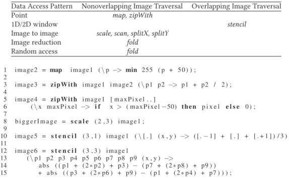
Table 1. Skeleton Functionality
Data Access Pattern Nonoverlapping Image Traversal Overlapping Image Traversal
Point map, zipWith
1D/2D window stencil
Image to image scale, scan, splitX, splitY
Image reduction fold
Random access fold
Fig. 1. Examples of image processing with stream-based skeletons.
2 RIPL DESIGN 2.1 RIPL Overview
RIPL is a DSL for describing FPGA designs for image processing algorithms at a very high level. RIPL’s design is inspired by stream-based functional programming languages (e.g., McGraw et al. (1985)) and libraries (e.g., Kiselyov (2012)), such asmapandzipWithover streams. Such primitives are sometimes calledskeletons(Cole1991), and this is how we refer to RIPL’s language primitives. RIPL skeletons capture many low- and medium-level image signal processing operations, such as 1D and 2D filters, image transformations, and global image reductions.
RIPL programs are nonterminating, repeatedly executed for every frame coming from a source. RIPL therefore must be able to process frames, ideally at the rate of capture. To achieve this, hard-ware pipelines are generated from RIPL programs to hide latency. Synthesizing intermediate data structures from high-level languages on FPGAs would quickly use up all available on-chip BRAM memory. Therefore, to maximize the use of BRAMs, RIPL skeletons are compiled to memory-efficient data-localized functions, such as pixel-to-pixel or region-to-region actor functions, rather than image-to-image actor functions, because the latter would incur high memory costs.
2.2 Image Processing With RIPL Skeletons
RIPL skeletons are reusable generalized image processing patterns, to which the user supplies functions and values. Their distinctions in terms of data access patterns are shown in Table1, with examples given in Figure1. Point operations, such as withmap, compute a single pixel value from an input pixel, and the processing does not depend on pixel neighbors (line 1 in Figure1). Examples include arithmetic, logical, and threshold operations. ThezipWithskeleton (line 3) merges two data structures—for example, two images or combining an image with a stream of a constant value (line 5).
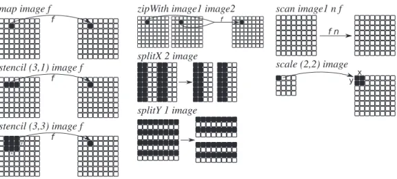
Fig. 2. RIPL skeletons.
Fig. 3. Visualizing image processing with RIPL’s stream-based skeletons.
Local operations, such as with stencil, depend on small 1D or 2D subregions of neighboring pixels (e.g., convolution, filtering, smoothing, image enhancements), upsampling an image with scale(line 8) with an interpolation filter withstencil, or horizontally splitting an image withsplitX. For example,splitX 2 img1would return two images, where the first is constructed from columns 1,2,5,6,9,10. . ., and the second image has columns 3,4,7,8. . ., and so on.
RIPL’s skeleton API is shown in Figure2. The user supplies functions and values, using standard notation for function type signatures. For example,mapis a skeleton that takes two arguments, an M×N image and function from a pixel to a pixel, and returns anM×N image. Images are read withimreadin row major order from left to right, then top to bottom. The typeP represents pixel integer values. An imageI(M,N) isM pixels in width andN pixels in height. Processing images with RIPL’s stream-based skeletons is visualized in Figure3.
2.3 Image Stencils, Recursion, and Random Access
2.3.1 Image Stencils.RIPL has a primitive for applying 1D and 2D stencils calledstencil. It cap-tures a way to express many common image processing kernels, such as a blur kernel and edge detection. Thestencilskeleton provides the user with the pixel values, and also the(x,y)position of the center pixel. Line 10 in Figure1is an implementation of a 1D blur stencil. For 1D stencils,
the syntax[.]points to the indexed columnwise position of that pixel. Indexing pixels on either side is done with+/-. For example,[.-1]points to the pixel to the left of the[.]pixel. When applying a 2D kernel, such as Sobel edge detection on line 12, thestencil (M,N) ..skeleton providesM∗N pixels to the user-defined function. When the user-defined kernel is applied at the edges of the image, the closest adjacent pixel is mirrored over the image’s edge. The(x,y)position argument can be used to make a choice about how to compute a kernel result for each position (e.g., applying different kernels for odd and even columns). This functionality is used for separating the low and high bands in a DWT in Section4.2.3:
2.3.2 Stateful Recursion.Thefoldskeleton is designed to meet algorithmic requirements that do not fit into RIPL’s stream combinator model. This skeleton supports the following:
— Accumulating state while traversingNdimensional data structures including images. — Random access intoNdimensional data structures.
— Recursion with thewhileconstruct.
Thefoldskeleton takes three arguments: (1) an initial state, (2) an iterable data structure, and (3) a user-defined function that takes a state and the next element from the structure, then executes a sequence of statements. The initial state can be a Boolean or integer literal, a tuple of literals, orNdimensional arrays created withgenarray, wheregenarray(50,10)creates a 50×10 array. An iterable data structure can either be a previously computed value, such as an image region, or an iterable range withrange, whererange(10,5)provides the user-defined function(i,j)loop counters.
Two examples usingfoldare the following:
The first computes the maximum pixel in an image. The user-defined function that applies themax binary operator is folded overimage1, starting from initial state 0. The second example instantiates a 1D array of size 256, to serve the purpose of a histogram data structure. The function folds over theimage1, incrementing the bin value positions according to each grayscale pixel value. 2.4 A Dataflow Intermediary for RIPL
RIPL programs are compiled to dataflow process networks (DPNs) (Lee and Parks2002) as an IR of image processing computations. A RIPL program is shown in Figure4, which normalizes an image’s grayscale distribution with its sum histogram. It reads image pixels withimreadinto a histogram withfold. A lookup table containing the scale factor is created withscanandmap. An output image is created from this lookup table. The arrows in Figure4(a) show the dataflow analysis that the RIPL compiler performs, to generate pipelined FPGA designs.
RIPL’s dataflow IR comprises static and cyclostatic properties to support the required schedul-ing behaviors of the RIPL skeletons. Synchronous dataflow (SDF) (Lee and Messerschmitt1987) actors produce and consume the same number of image pixels on every firing. Skeletons map andzipWithare compiled to SDF actors. All other skeletons are compiled to cyclostatic dataflow (CSDF) (Bilsen et al.1996) actors. They have cyclically changing state transition sequences and have an internal actor state for pixel/line buffers to support 1D/2Dstencil,scale,scan,splitX,splitY, andfold. The scheduling behavior of each CSDF actor for RIPL skeletons is fixed, and the pixel/line
Fig. 4. RIPL dataflow analysis of histogram normalization.
buffer sizes and the functions to produce data output values are derived from the user’s RIPL code. The dataflow IR exploits FPGA parallelism and good data locality.
Parallelism. The dataflow model of independent computational blocks are a natural fit for paral-lel FPGA circuits, to process infinite image streams. Paralparal-lelism is implicit in RIPL, without paralparal-lel primitives or pragmas. Generating hardware pipelines hides latency. The RIPL compiler preserves lazy evaluation in the tail of image streams to exploit pipelined parallelism. Otherwise, actors would consume more data than needed to compute their function, which would reduce paral-lelism and increase memory costs for intermediate storage. There are two forms of automatic RIPL parallelism:
—Temporal parallelism. This form of parallelism is introduced when image data is streamed through a pipeline of producer-consumer kernels (e.g., the output from astencilis the input to azipWithoperation).
—Spatial parallelism. RIPL produces computational code inside actors to exploitspatial paral-lel FPGA logic. Paralparal-lelism is exploited within expressions in user-defined functions, in the absence of dataflow dependencies within expressions.
Data locality. There is no global shared memory in the dataflow model. Instead, the dataflow memory model is that of isolated memory within actors, where computations and their data are co-located. This maps naturally to on-chip contention-free (i.e., parallel accesses) BRAM memory and registers distributed across FPGA fabric.
3 RIPL IMPLEMENTATION
Each RIPL skeleton is compiled to a dataflow actor that encapsulates a finite state machine (FSM), responsible for the required scheduling behavior, and a corresponding datapath. These actors are connected into deep parallel pipelines as multiple skeletons are used in larger programs. RIPL enforces single assignment semantics (i.e., a variable is assigned a value with a skeleton instance exactly once). This makes data dependencies easy to extract to dataflow wiring, to facilitate the generation of hardware pipelines. The RIPL compiler is open source,1and the RIPL, CAL, and C++ implementations for the evaluation in Section4are available as an open dataset (Stewart2018). 3.1 Skeletons to Dataflow FSMs
3.1.1 Dataflow Semantics for RIPL Skeletons.The compilation of each RIPL skeleton is based on a framework for describing rule-based dataflow actors (Janneck2003). It describes the data rates and static scheduling for each RIPL skeleton in terms of transitions on an abstract machine, which
is later compiled to hardware specified in Verilog (Section3.2). An actor is a sequential process, communicating values by transitioning between states in the actor’s FSM. The state machine re-ceives tokens and reacts to them, possibly entering another state, and possibly producing tokens. A state transition fromσ toσconsumes a tuplesof token sequences and produces a tuplesof token sequences. An actor has a set ofminput ports, writtenSm, andnoutput ports, writtenSn. The valuemis dictated by the arity of the corresponding RIPL skeleton. For example,zipWithtakes two images as inputs, and hencemis 2 for this skeleton. If the output of one skeleton is used as an input argument of multiple other skeletons, then those actors are connected to the same input port and the stream is automatically duplicated into each connection.
LetU be the universe of all values, and letS=U∗be the set of all finite sequences inU. A tuple s∈Smcontains one or more token sequences consumed frompports, where 1p m. We write
sAp to describe a token sequence of lengthAat portp. For example, a transition fromσtoσthat consumes sequences from input ports 1 and 2 of lengthsAandB, to produce a sequence of length Cto an output port 1, is written as follows:
σ s 1 A×sB2→s1C
−−−−−−−−−→σ
For some scheduling phases of a RIPL skeleton, a transition rule may not read from or write to any ports. We use∅as port descriptions for these transitions. To support the stateful RIPL skeletons such asstencil, an internal actor state is needed. We addSas a notation to transition rules for the internal actor state. State transition examples are written as follows:
σ0,S
s1 3→s16
−−−−−→σ1,S
This transition moves from FSM stateσ0with a set of internal variable states inSto FSM stateσ1 with internal variable statesS, and consumes three input tokens from input port 1 and emits six output tokens to output port 1. In the mapping from RIPL to dataflow graphs, the vertices (actors) represent image operations and the edges (wires) represent dataflow between composed skeletons.
3.1.2 Compilation Scheme.
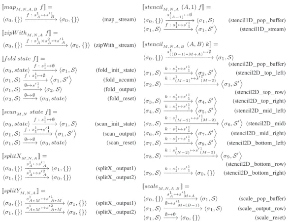
Pointwise skeletons. The skeleton to dataflow FSM compilation scheme is shown in Figure5. Each skeleton is compiled to an actor with one or more transitions. ThemapandzipWithskeletons are each compiled to a single transition rule in an SDF actor with no internal state—that is, transition rules(map_stream)and(zipWith_stream)map from an empty internal state{}to an empty internal state, and the output values from these transitions are determined by the user-defined functionf. Image transforms. Thescaleskeleton is compiled to three transition rules. The(scale_pop_buffer) consumes a row and outputs each pixel in turn by the width scale factorM. The(scale_output_row) outputs this scaled rowN −1 times, whereN is the height scale factor, then the FSM is reset toσ0 with transition(scale_reset). Thescanskeleton is compiled to three transition rules. The(scan_init_ state)rule initializes the actor buffer with the user-defined initial state. The(scan_output)rule per-forms the accumulation operation, outputting intermediate values until a data structure is con-sumed, then(scan_reset)reset back to the initial state. ThesplitXskeleton has two rules, one each for outputting to output ports 1 and 2. ConsideringsplitX 2 image,(splitX_output1)consumes two tokens and then outputs them to output port 1, then(splitX_output2)does the same, outputting to output port 2. This alternating schedule repeats forever. The same FSM schedule is used forsplitY, this time consuming entire rows in each transition.
Stencils. A 1D image blur stencil in Figure6demonstrates how the RIPL compiler minimizes the memory requirements of an FPGA. The compiler infers the range of the indexed pixel either side
Fig. 5. Compilation scheme from RIPL skeletons to actor FSMs.
Fig. 6. Circular buffer to supportstencil (3,1) ..for a 1D blur kernel.
of [.], which in this case is three pixels between [.−1] and [.+1]. The actor contains a three-element array that acts as a circular buffer, which is partially filled with two three-elements by firing rule(stencil1D_pop_buffer)to reach stateσ1and a mid position pointer is set to 1. Each time the
(stencil1D_stream)rule is fired, the next incoming token is pushed to the front of the buffer, and the RIPL function is computed on the buffer’s contents as the output token value, and the mid position pointer is rotated forward one position. This stencil actor needs memory for just four pixels, the three-element circular buffer and the incoming token, to apply a 1D blur over an entire image.
Thestencilskeleton for 1D stencils is compiled to two transition rules. The internal state for 1D stencils is populated with the(stencil1D_pop_buffer)rule before transitioning to stream-based rules(stencil1D_stream). Thestencilskeleton for 2D stencils is compiled to 10 transition rules. The (stencil2D_populate_buffer)rule consumes the first two rows andApixels required to start pro-cessing an image from the top left corner—that is, by consuming((B−1)∗M+A)tokens where
Fig. 7. RIPL skeleton transition execution examples.
AandBare the width and height of the kernel window andMis the width of the entire image. The remaining 9 rules carry out three tasks: (1) consume one pixel into the internal state, (2) com-pute the application of the user-defined 2D kernel function f on the window around the central pixel, and (3) output that computed value. They are defined as separate transition rules to index the internal state to handle boundary conditions at image edges, where the edge pixel is mirrored over the boundary.
Reductions and stateful recursion. Thefoldskeleton is compiled to four transition rules. The inter-nal actor state is persisted throughout the consumption of each input data structure (e.g., an image region). The internal state buffer is initialized with the user-definedstatevalue before being mod-ified each firing with(fold_accum). Once an entire data structure is consumed, the(fold_output) rule begins firing to output the final state. The(fold_reset)resets the internal actor buffer to the initial state and readies the actor to consume the next data structure.
3.1.3 Example Transitions.The execution of RIPL skeletons is now given showing sequences of
FSM rule firings for two examples, shown in Figure7. The first example combines two images with zipWith, with the mean of six pixels at the same position in each image. The second example uses foldto return the maximum pixel value in a 2×2 image region, by repeatedly folding the current highest pixel value through the image until all pixels have been consumed. The initial internal state takes the second argument to the skeleton, in this case 0. This is used to retain the largest current pixel value while consuming, then immediately discarding, each pixel from the image. Once all pixels have been consumed, the internal state is output with(fold_output)before the FSM is reset toσ0,0 for the next image frame.
3.2 Dataflow to FPGAs
The CAL dataflow language (Eker and Janneck2003) is the target language of RIPL’s dataflow IR backend. There are three phases to compile RIPL to FPGAs: (1) compiling RIPL to CAL, (2) compiling the dataflow graph to Verilog, and (3) synthesizing the Verilog to a bitfile. The dataflow intermediary provides optimization opportunities (e.g., Stewart et al. (2017)) before being compiled to hardware components such as registers, memories, and actor communication hand-shake protocols. Xronos (Bezati2015), an FPGA backend plugin for the Orcc compiler, maps each actor into a language-independent model (LIM) and connects each LIM block to a clock. Xronos is designed to support dynamic asynchronous dataflow and therefore adds a FIFO-based data com-munication mechanism to support token passing. Decoupling actor comcom-munication via these FI-FOs results in two clock cycles latency per pixel—that is, for a 512×512 image at 100MHz, the highest theoretical performance is 512100000000×512×2 =191 FPS for a single actor performing elementwise
Fig. 8. Thresholding with a maximum pixel value in HLS OpenCV.
operations. The Xilinx OpenForge compiler allocates hardware: memory, arithmetic datapaths, registers, and actor interconnects, then generates HDL modules for each actor and for defining dataflow connectivity between these modules. This HDL code is synthesized and deployed to FP-GAs using commercial tools.
RIPL’s code generation strategy maximizes spatial parallelism to maximize the number of oper-ations per clock cycle. By default, OpenForge uses BRAM blocks for CAL arrays beyond a certain size. Our experiments with OpenForge show that a BRAM block is instantiated for CAL arrays requiring more than 2KB of storage (e.g., about a 4×512 row buffer at 8 bits per pixel). To use a BRAM in the combinational setting, at most two read/write accesses to a CAL array may occur. When more than two reads/writes are performed on the same array in an actor’s action, OpenForge instead instantiates LUTs for CAL arrays with three-plus reads/writes to preserve zero latency accesses.
4 EVALUATION
4.1 RIPL Versus HLS OpenCV
4.1.1 Expressivity.Vivado HLS OpenCV (Neuendorffer et al.2015) is a collection of 34 prede-fined functions, a subset of the 2,500+ algorithm functions in OpenCV for CPUs. An example is shown in Figure8. In contrast, RIPL provides algorithmic templates, whose functionality is en-tirely user defined. For example, the HLS OpenCVhls::Maxfunction for combining two images can be expressed with RIPL’szipWith. HLS OpenCV’shls::Filter2Dis a convolution filter. RIPL’s stencilsupports any stencil function, including convolution. This demonstrates the inflexibility of libraries of fixed kernels. Moreover, the library approach prohibits optimizations across library call boundaries. Other expressivity differences are the following:
—Sharing. Since theMattype is just a synonym forhls::streamin the HLS OpenCV library, a hls::Duplicatecall must be performed on an image to ensure that the underlying data stream is not consumed in one program location to deadlock in another location. RIPL supports automatic image sharing, where an image is processed in two places in a program.
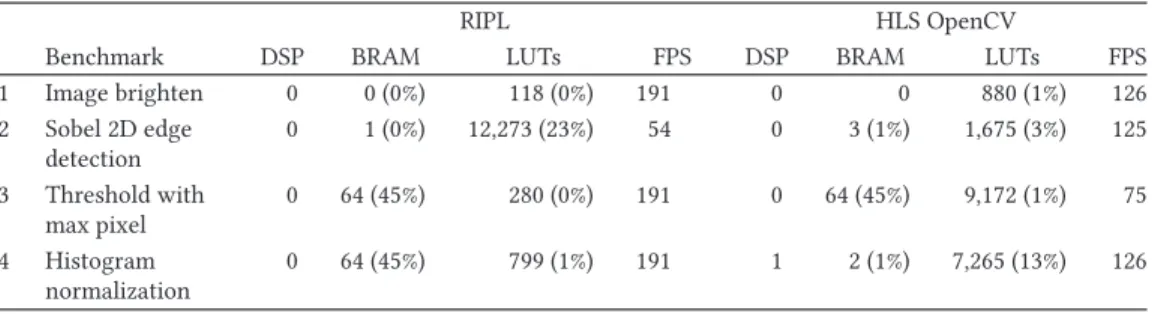
Table 2. Microbenchmark Results
RIPL HLS OpenCV
Benchmark DSP BRAM LUTs FPS DSP BRAM LUTs FPS 1 Image brighten 0 0 (0%) 118 (0%) 191 0 0 880 (1%) 126 2 Sobel 2D edge detection 0 1 (0%) 12,273 (23%) 54 0 3 (1%) 1,675 (3%) 125 3 Threshold with max pixel 0 64 (45%) 280 (0%) 191 0 64 (45%) 9,172 (1%) 75 4 Histogram normalization 0 64 (45%) 799 (1%) 191 1 2 (1%) 7,265 (13%) 126
—Image shape inference. OpenCV programming requires explicit dimension in image decla-rations. For example,hls :: Mat512,512,HLS_8U C1 defines a 512×512 single channel image, using eight unsigned bits per pixel. In contrast, the RIPL compiler infers the dimen-sion of every intermediate image, by following dimendimen-sion transformations performed by skeletons through the implicit dataflow paths starting fromimread, where dimensions are specified.
—Parallel pipelines. Pipelining in RIPL is automatic. For example, streaming the result of a mapin astencilwill generate a hardware pipeline. In HLS OpenCV, the programmer must specify#pragma HLS dataflow above the function calls intended to be pipelined over the image stream.
4.1.2 Performance Comparison.We use four benchmarks to compare the space performance of
RIPL and OpenCV compiled to FPGAs using Vivado HLS (Xilinx2017b). Programs are compiled for the Xilinx Zedboard XC7Z020 for 512×512 single-channel images. The post place-and-route results in Table2are taken from Stewart et al. (2016). To quantify computational image processing performance, we use RTL simulation to calculate latency in clock cycles per 512×512 frame and report FPS according to the clock frequency. All experiments were performed using a 100MHz clock, which is the default frequency for Vivado HLS, and we did not perform any speed optimiza-tions on Vivado HLS or RIPL-generated code.
RIPL achieves a higher FPS performance compared to HLS OpenCV, achieving 191 FPS for im-age brightening, max-thresholding, and histogram normalization. This is the maximum achievable FPS result for RIPL at 100MHz (i.e.,512100000000×512×2), due to FIFO-based token passing latency introduced by RIPL’s FPGA backend. OpenCV achieves 126, 75, and 126 FPS, respectively. HLS OpenCV out-performs RIPL for a Sobel 2D edge detection, 125 FPS versus 54. This may be caused by the amount of runtime scheduling caused by the 10 dataflow transition rules in the implementation ofstencil (Section3.1.1) to handle mirroring pixels over boundaries. Reducing runtime scheduling by reduc-ing the number of transition rules forstencilis future work. Resource utilization is similar, except for Sobel, where RIPL uses two BRAM blocks less and a lot more LUTs (23%). Because CAL code generated by RIPL implements a combinational filter (Section3.2), accessing up to nine different data at the same time to compute Sobel, OpenForge is unable to map the data into BRAMs, which are limited to two simultaneous read/writes. Hence, data storage is mapped to LUTs.
HLS OpenCV uses less BRAM than RIPL for histogram normalization. The dataflow graph gen-erated from RIPL computes two passes of the image: one to compute the histogram and a second to normalize the color distribution with it. In contrast,hls::EqualizeHist()normalizes a frame using a histogram computed for the previous frame. This approximation optimization means that BRAM is not needed to store an image for the second pass to normalize with the computed histogram.
its neighbors including the pixel itself and commonly realized by convolving with a predefined mask (González and Woods1992). An equation for such filters is expressed as follows:
I=W ∗I = N n=1 M m=1 w(m,n)·I(m,n), (1)
whereIis the input image of sizeM×N,Iis the filtered image,W is the filter kernel,mandnare the pixel locations, and∗is a convolution operator. The process is repeated using a sliding window to receive filter output for the entire image. Average filtering with filter coefficientsw(m,n)=19 can be implemented as a RIPL function using thestencilskeleton:
4.2.2 Intermediate-Level Image Processing: Multiresolution 2D Wavelet Transform.DWT is used
for many image processing applications, such as compression, denoising, and texture analysis. Multiorientation and multiresolution analysis using DWT closely resembles human vision. DWT decomposes an image into independent frequency subbands of multiple orientations at multiple scales demonstrating details and structures. Due to its popularity in the JPEG2000 image com-pression standard (Taubman and Marcellin2012), we use the 5/3 wavelet kernel as our RIPL ex-ample, using a lower-complexity lifting-based approach. The filters are realized by decomposing the signal into lifting steps by factoring its polyphase matrix using the Euclidean factoring algo-rithm (Daubechies and Sweldens1998). The input signal, lowpass subband signal, and highpass subband signal are denoted asa[n],s[n],andd[n],respectively. DWT is expressed in Equation (2), wheres0[n]a[2n] andd0[n]a[2n+1]:
5/3⎧⎪⎨⎪ ⎩
d[n] =d0[n]−12(s0[n+1]+s0[n]), s[n] =s0[n]+14(d[n]+d[n−1]).
(2) A 2D DWT is computed by separately filtering rows and columns leading to one approximation (LL) subband and three detailed subbands in the decomposition leveli∈N1 emphasizing verti-cal (LHi), horizontal (HLi), and diagonal (HHi) contrasts within an image, portraying prominent
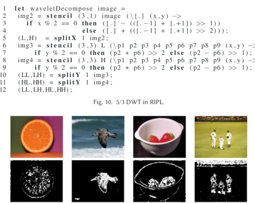
edges in various orientations as shown in Figure9. This process is repeated on the LL subband to get multiresolution decomposition. The 5/3 DWT is implemented as a RIPL function in Figure10. TheLandHcomponents of the inputimageare computed withstencilon line 2 and then separated toLandH usingsplitXon line 5. TheLL,LH,HL,andHH subcomponents are computed in the vertical direction in the same fashion on lines 6 and 8, and separated on lines 10 and 11.
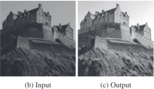
4.2.3 High-Level Image Processing: Visual Saliency Modeling.The human visual system is
sen-sitive to many salient features that lead to attention being drawn toward specific regions in a scene. A visual attention model identifies the salient regions in an image as perceived by human
Fig. 9. Example of multiresolution wavelet decomposition, where (b), (c), (d), and (e) are level 1 approximation (LL1), vertical (LH1), horizontal (HL1), and diagonal (HH1) subbands, respectively.
Fig. 10. 5/3 DWT in RIPL.
Fig. 11. Example saliency maps computed by the original model: row 1 shows original images, and row 2 shows the thresholded saliency maps generated by our implementation.
vision and has applications in many domains including computer vision (Borji and Itti2013). We have adopted the visual attention model from Bhowmik et al. (2016), which demonstrates superior performances in joint saliency detection and low computational complexity. The algorithm uses the 5/3 DWT in Section4.2.2as its core decomposition. Example algorithm results are shown in Figure11.
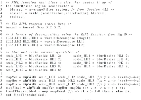
DWT captures horizontal, vertical, and diagonal contrasts within an image, respectively, por-traying prominent edges in various orientations. A complete visual saliency RIPL implementation is shown in Figure12, which uses thewaveletDecomposeRIPL function from Figure10. It processes theYchannel of theYU V color spectral space, because this luminance channel exhibits prominent intensity variations and has significant structural information of the scene and carries maximum weight in the original algorithm. The RIPL implementation applies three levels of wavelet decom-position. Due to the dyadic nature of the multiresolution wavelet transform, the image resolutions are decreased after each wavelet decomposition iteration from lines 11 to 13. This is useful in
cap-Fig. 12. Visual saliency in RIPL.
turing both short and long structural information at different scales. TheblurResizefunction on line 2 is called on lines 16 through 20, which applies an average filter to each subband to remove unnecessary finer details, then scales up the result back to a full resolution output. The interpolated subband feature maps,lhi (horizontal),hli(vertical), andhhi (diagonal),i ∈N1, for all decomposi-tion levelsL1 to 3 are combined by a weighted linear summation as illustrated in Equation (3):
lh1···LY = L i=1 lhi∗τi hl1···LY = L i=1 hli ∗τi, hh1···LY = L i=1 hhi∗τi , (3)
whereτi is the subband weighting parameter andlh1···LY,hl1···LY andhh1···LY are the subband feature maps for the spectral channelY, on lines 22 through 24.
Last,SY, the saliency map for theY spectral channel, is on line 25 and is computed as follows,
before being thresholded with a binary threshold to emphasize salient regions:
SY =lhY +hlY +hhY. (4)
4.2.4 Visual Saliency Results.
RIPL versus C++ for hardware. The RIPL visual saliency implementation is compared to variants of an equivalent C++ implementation. The C++ implementation separates the three algorithmic components into C++ functions: the blur filter, the FWT, and the weighted linear summation. C++ templates are used to size array arguments to these functions, and these arrays are updated in-place in the body of each function. These template parameters are propagated through the program at compile time from 512 and 512 height and width image dimensions in the test bench—for example,
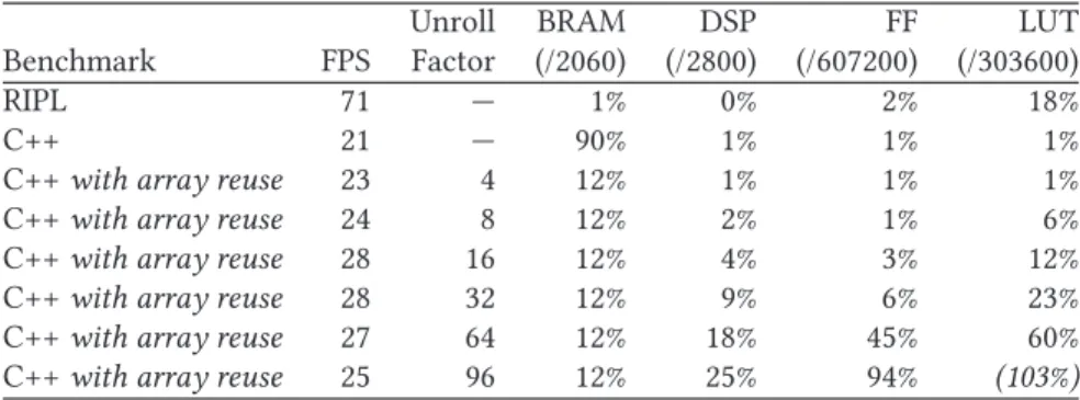
Table 3. Visual Saliency on a Virtex 7
Unroll BRAM DSP FF LUT
Benchmark FPS Factor (/2060) (/2800) (/607200) (/303600)
RIPL 71 — 1% 0% 2% 18%
C++ 21 — 90% 1% 1% 1%
C++with array reuse 23 4 12% 1% 1% 1%
C++with array reuse 24 8 12% 2% 1% 6%
C++with array reuse 28 16 12% 4% 3% 12%
C++with array reuse 28 32 12% 9% 6% 23%
C++with array reuse 27 64 12% 18% 45% 60%
C++with array reuse 25 96 12% 25% 94% (103%)
The C++ variants are the following:
(1) C++ with array reuse. Each function contains declared 2D arrays with element values ini-tialized to zero. For example,lowBand[h][w/2]andhighBand[h][w/2]are declared in the waveletDecomposefunction, which can both be populated in a single loop statement to separate the low and high bands in one iteration over the image. This version contains 27 arrays.
(2) C++ with extensive reuse of arrays. This version reuses some arrays for different pur-poses. Refactoring has been done manually—for example, renaminglowBand[h][w/2]to band[h][w/2]and populating it with low band FWT values to compute LL and LH, be-fore repopulating it with high band values to compute HL and HH. This approach also sequentializes the summation of weighted LH, HL, and HH contrasts because one array is repopulated with LH, then HL, then HH, after each sum accumulation into an output array. This version contains 13 arrays.
(3) C++ with array reuse and loop unrolling. Loop unrolling with#pragma AP unrollis em-ployed to create multiple parallel independent operations from originally sequential loops. This loop unrolling pragma is used in eight places, and the unrolling factor is varied to measure the trade-off between space and latency.
Hardware designs for RIPL and C++ are clocked at 100MHz for the Virtex 7 VC707 and syn-thesized using Vivado 2016.2. Results are displayed in Table3. Vivado HLS does not apply fusion optimizations to eliminate intermediateforloops over successive arrays, and hence the 90% BRAM use for 27 image buffers. Manually eliminating intermediate arrays down to 13 reduces BRAM use to 12%, which runs at 23 FPS. Unrolling the eightforloops in the C++ code up to an unroll factor of 32 increases FPS to 28, and increases DSP, FF, and LUT resource use. FPS performance degrades as more space is needed with a 64 unroll factor, and an unroll factor of 96 requires too many LUTs. The RIPL program achieves 2.5x higher FPS performance than the best C++ variant at 71 FPS, using fewer BRAMs and a similar number of LUTs.
RIPL versus dataflow in software. The RIPL program has also been compiled for an Intel i5 3.2GHz CPU, using the Orcc dataflow compiler’s C backend. This CPU is a high-end processor compared to embedded processors usually used for remote image processing. The CPU visual saliency per-formance is 9 FPS. The FPGA perper-formance is 8.3x faster than the CPU.
Code size. Visual saliency is 29 lines of RIPL code. The C++ visual saliency is 160 lines of code, and 162 with manual array reuse—that is, RIPL is 5x shorter than the C++ equivalents. The 29 lines of RIPL are compiled to 44 actors amounting to 3.1k lines of dataflow actor code generated by the
This has been applied to text detection in images (Kim et al.2003) and real-time video tracking of nonrigid objects (Comaniciu et al.2000). Because the algorithm is used to distinguish between objects based on their color rather than shape, nonrigid objects can be tracked. The applications in image segmentation were proposed in Comaniciu and Meer (1999).
4.3.1 Mean Shift Segmentation Algorithm.Each pixel is mapped into an RGB color space, where
each pixel has a vector position according to its red, green, and blue values. This feature space can be regarded as the probability density function of color. Dense regions of this space correspond to the local maxima of the probability density function. The value of a density function at a point is estimated from the values observed around that point. The multivariate kernel density estimator at the pointxestimates the value using points within radiushofxand is given by
ˆ fh,k(x) = ck nhd n i=1 k x−hxi 2 . (5)
The density gradient estimator at a point can be estimated similarly from the values within a small window around the point. The modes of the density estimator are found at the points with zero gradientf(x)=0. The mean shift vector given by
mh,k(x) = 1 2h 2cˆfh,k(x) ˆ fh,−k(x) = n i=1xik(||x−hxi||2) n i=1k(|| x−xi h ||2) −x (6)
is the difference between the weighted mean of points within the bandwidth parameterhandx, the center of the window. It points in the direction of a normalized maximum density gradient estimate; it is zero at the point where the gradient of the probability density function is zero. The mean shift vector can therefore be used to define a path toward the local maximum of the estimated density for each point in the feature space. To ensure that mean shift clustering is applied only to neighboring image pixels of similar RGB colors, the mean shift vector is rewritten as follows:
mhr,hs,G(x)= n i=1x r,s i k(|| xr−xr i hr || 2)k(||xs−xsi hs || 2) n i=1k(|| xr−xr i hr || 2)k(||xs−xsi hs || 2) − x, (7)
wherexr,s is the 5D position in the joint space,xr is the 3D component of the joint space vector
corresponding to the range, andxs is the 2D component of the joint space vector corresponding to the position in the image. Using the Epanechnikov kernel, the required value,
−k x−x h = 1 0≤x−x≤h 0 x−x>h, (8)
determines that all pointsxwithin a radiushofxare considered in the calculation, and all points outside are not. The algorithm is shown in Algorithm 1. For each point in the joint space:
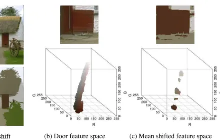
Fig. 13. Mean shift segmentation visualized.
(1) Define a spherical window of radiushr around the three color dimensions of this point
and a circular window of radiushs around the spatial dimensions, and calculate the mean
shift vector (Equation (7)) from this point.
(2) If the mean shift vector is nonzero, add it to the current position and go back to step 1. (3) If the mean shift vector is zero at this point, define this point as the peak of the original
point.
All points with the same peak are considered to belong to the same cluster. ALGORITHM 1:Mean Shift Clustering Algorithm Pseudocode
input:Image file
output:Image with each cluster shaded the color of its peak 1 foreach index in joint space arraydo
2 whilepeak has not been found & iteration limit not exceededdo 3 Collect points within the spatial window
4 Collect points within the range window 5 Calculate mean shift vector using Equation (7) 6 ifmean shift vector is zerothen
7 Peak has been found;
8 end
9 Add mean shift vector to current point in joint space;
10 end
11 Store value of peak in equivalent index of output image; 12 end
Mean shift segmentation of image #385028 from the Berkeley segmentation training dataset (Martin et al.2001) is shown in Figure13. Figure13(b) shows the feature space for the red door, and Figure13(c) shows the segmented colors in the feature space after mean shift.
Fig. 14. Mean shift segmentation in RIPL.
4.3.2 Mean Shift Segmentation in RIPL.The RIPL implementation is split into three phases,
shown in Figure14. The first phase reads an RGB image into the first three elements in the third dimension of apeaksRGBarray. The fourth and fifth elements store the 2D image space coordinates. The second phase performs the mean shift kernel, which recurses withwhileeither until mean shift has converged to a peak or until the recursion limit is reached. Thefoldoverrange(512,512)iterates (i,j)counters, and the kernel creates a window around this point. A center of mass is computed for each point in the window, and each peak value is updated. If the current point is the peak (peakFound), the whileloop exits. The third phase projects the mean shifted RGB values from elements 1 to 3 of the third dimension ofpeaksRGBas output of the program.
Fig. 15. Deploying RIPL to image processing architectures.
4.3.3 Mean Shift Segmentation Results.Mean shift in RIPL is synthesized at 100MHz for the
Virtex 7 VC707. The mean shift convergence limit is 5, the spatial window size is 10, the range window is 20, and test image size is 512×512. The RIPL is 70 lines of code. This compiles to 700 lines of dataflow IR code, which compiles to 427k lines of HDL code. The HDL uses 2% of available LUTs, 1% FFs, 1% DSPs, and 91% BRAMs. The BRAMs are used for the 3D array that stores the RGB values and the 2D image space coordinates. The RIPL mean shift program achieves approximately 7 FPS. This compares to our equivalent C++ that achieves 1.1 FPS for the mean shift kernel, or 0.7 FPS when factoring in image file IO, parallelized with OpenMP on 64 cores of an AMD Opteron 1.4GHz CPU.
4.4 Evaluation Platform: RIPL to an FPGA-Based Smart Camera
To evaluate RIPL on real-time architectures, the Xilinx Zedboard in Figure15(b), a platform FPGA based around the Zynq-7020 chip, is used. Only the result of RIPL programs are transmitted over Ethernet or Wifi, rather than raw camera frames, avoiding pressure on network bandwidth and power needed for data transmission. Our experimental setup in Figure15(a) integrates camera control and image acquisition hardware, interfacing an off-chip OmniVision OV7670 sensor, and a host processor interface. Xillybus2is used to abstract the interface between hardware and soft-ware (Andrews et al.2004), ensuring that our FPGA subsystem is portable across Zynq platforms. The interface converts hardware FIFO channels to file descriptors in software, allowing software to use standard libraries to receive data from the FPGA for further processing, or to transmit RIPL results over a network connection. A complete description of the architecture is given in Bhowmik et al. (2017).
5 RELATED WORK
In addition to RIPL, two other high-level image processing FPGA languages have been developed in recent years: Darkroom (Hegarty et al.2014) and Rigel (Hegarty et al.2016). A comparison of their compilation to FPGAs is shown in Figure16.
The expressivity of Darkroom is constrained to functions from(x,y)coordinates to pixel val-ues (i.e., elementwise operations) and stencils that use pixels neighboring an(x,y)position. Dark-room is compiled to a line buffer IR; however, its line buffer IR to Verilog compiler is not publicly available. Darkroom is limited to processing one pixel per clock (Hegarty et al.2016), a limitation overcome by its successor, Rigel. Rigel is a line buffer compiler IR language rather than a user fac-ing language like RIPL or Darkroom. It presents a space/time trade-off to the user and overcomes a limitation of Darkroom by supporting the construction of image processing pyramids. Image pyramids are also supported by RIPL, as shown in the three-level DWT example in Section4.2.2. Like RIPL, Rigel supports SDF dataflow semantics, with an extension that supports dynamic clock cycle latency and dynamic scheduling to check the validity of inputs. A contribution of our
Fig. 16. Compilation of high-level FPGA image processing languages.
article in Section3.1is a formal account of the FSMs in the SDF and CSDF models that support RIPL’s skeletons. Rigel supports data-dependent early kernel termination, which Hegarty et al. (2016) callsparse computations. RIPL also supports data-dependent latency from image processing kernels with thewhileconstruct.
A key difference between RIPL and Darkroom/Rigel is RIPL’s support for multiple passes. For example, the histogram normalization RIPL program in Figure4folds over an image to compute an image histogram before normalizing pixels of the original image with that histogram. This would require two passes in Darkroom/Rigel, with a handwritten driver to combine the designs.
Another approach is FPGA support for the Halide (Pu et al.2017) stencil language, with a back-end targeting C that is synthesizable with Vivado HLS. The language separates computation from scheduling. To achieve FPGA parallelism, loops should be manually unrolled with Halide’sunroll by increasing the degree of parallelism of the FPGA datapath. In contrast, parallelism is automat-ically derived from pipelines of RIPL skeletons, and data locality is achieved with RIPL’s stream combinator programming style. To support FPGAs, the Halide programming model differs slightly from its software origins. The parallelism primitives (e.g.,tileandvectorize) are not supported by the FPGA backend. As such, existing Halide code may have to be modified to run on FPGAs.
Darkroom, Rigel, and Halide are all restricted to expressing image stencil computations. RIPL supports elementwise stencils with stream combinatorsmap,zipWith, andscale, and 1D/2D win-dow stencils with thestencilskeleton. RIPL’sfoldskeleton adds expressivity needed for image reduction operations, and recursive algorithms with nonlocal access patterns, as demonstrated with mean shift segmentation in Section4.3. The Rigel work (Hegarty et al.2016) suggests that Rigel’s higher-orderReducemodule supports binary reduction only on windowed kernels residing in line buffers and not on entire images. RIPL’s fold skeletons can reduce image regions and also entire images.
A different approach to FPGA design is the use of graphical interfaces, where IP blocks are con-figured and connected to generate the target system. Most notable is the Matlab/Simulink HDL Coder (MathWorks2017), which is supported through vendor FPGA-specific technologies, namely Xilinx System Generator for DSP (Xilinx2017a) and Altera DSP Builder (Altera2017). This ap-proach is used for rapid prototyping with fast development cycles, as IP blocks are ready to use. However, the black box nature of most IP blocks limits functionality customization, so algorithm changes are prohibited if the desired modified functionality does not exist in IP block toolboxes. In contrast, textual languages such as RIPL provide the opportunity for programmers to define custom functionalitywithingenerated IP blocks (e.g., as user-defined skeleton functions in RIPL). 6 CONCLUSION
This article presents RIPL, an image processing language for FPGAs. The language has high-level algorithmic skeleton primitives that capture image processing requirements including 1D/2D
stencils, as well as random data access and recursion. The skeletons are abstractions that represent small programmable IP block templates that form building blocks for constructing higher-level al-gorithms. We show RIPL’s expressivity for filters, a wavelet transform, and a pyramidal visual saliency algorithm in Section4.2, and mean shift segmentation in Section4.3. RIPL is more ab-stract than OpenCV for small microbenchmarks because parallelism, data types, FIFO depths, and data copying are inferred. Despite this, RIPL outperforms in three of four benchmarks. RIPL also outperforms a C++ equivalent for visual saliency compiled with Vivado HLS.
There are many compilation routes for high-level FPGA languages (Section5), such as compiling generic dataflow or domain-specific IRs, and direct routes to RTL. This presents a trade-off between compile-time reasoning about throughput and fine-grain pixel processing pipelines, and real-world expressivity. RIPL’s generic dataflow IR underpinnings allow it to support random global data ac-cess, recursion, and automatic parallelism, in addition to standard image stencil pipelines. Low-ering image processing information from RIPL into its IR will enable fine-grain scheduling (e.g., adapting line buffer pipelines as in Rigel’s IR). Likewise, adding recursion, dataflow feedback, and global data access to Rigel’s IR, likely at the cost of compile-time pipeline scheduling, will expand its expressivity for complex vision algorithms. Tying flexible dataflow semantics (for expressivity) with image processing IRs (for optimization) could enable user-driven rewrite systems (e.g., Jones et al. (2001)) to expose space versus time FPGA trade-offs guided by acceptable domain-specific approximations.
REFERENCES
S. Ahmad, V. Boppana, I. Ganusov, V. Kathail, V. Rajagopalan, and R. Wittig. 2016. A 16-nm multiprocessing system-on-chip field-programmable gate array platform.IEEE Micro36, 2, 48–62.
Altera. 2017. DSP Builder for Intel FPGAs. Retrieved February 4, 2018, from https://www.altera.com/products/design-software/model---simulation/dsp-builder/overview.html.
David L. Andrews, Douglas Niehaus, Razali Jidin, Michael Finley, Wesley Peck, Michael Frisbie, Jorge L. Ortiz, Ed Komp, and Peter J. Ashenden. 2004. Programming models for hybrid FPGA-CPU computational components: A missing link.
IEEE Micro24, 4, 42–53.
Endri Bezati. 2015.High-Level Synthesis of Dataflow Programs for Heterogeneous Platforms: Design Flow Tools and Design Space Exploration. Ph.D. Dissertation. School of Engineering, Ecole Polytechnique Federale de Lausanne, Switzerland. Endri Bezati, Simone Casale Brunet, Marco Mattavelli, and Jörn W. Janneck. 2016. High-level synthesis of dynamic dataflow
programs on heterogeneous MPSoC platforms. InProceedings of the International Conference on Embedded Computer Systems: Architectures, Modeling, and Simulation (SAMOS’16). IEEE, Los Alamitos, CA, 227–234.
Deepayan Bhowmik, Paulo Garcia, Andrew M. Wallace, Robert J. Stewart, and Greg Michaelson. 2017. Power efficient dataflow design for a heterogeneous smart camera architecture. InProceedings of the 2017 Conference on Design and Architectures for Signal and Image Processing (DASIP’17). IEEE, Los Alamitos, CA, 1–6.
Deepayan Bhowmik, Matthew Oakes, and Charith Abhayaratne. 2016. Visual attention-based image watermarking.IEEE Access4, 8002–8018.
G. Bilsen, M. Engels, R. Lauwereins, and J. A. Peperstraete. 1996. Cycle-static dataflow.IEEE Transactions on Signal Processing
44, 2, 397–408.
Ali Borji and Laurent Itti. 2013. State-of-the-art in visual attention modeling.IEEE Transactions on Pattern Analysis and Machine Intelligence35, 1, 185–207.
André Rigland Brodtkorb, Christopher Dyken, Trond Runar Hagen, Jon M. Hjelmervik, and Olaf O. Storaasli. 2010. State-of-the-art in heterogeneous computing.Scientific Programming18, 1, 1–33.
Manuel M. T. Chakravarty, Gabriele Keller, Sean Lee, Trevor L. McDonell, and Vinod Grover. 2011. Accelerating Haskell array codes with multicore GPUs. InProceedings of the POPL 2011 Workshop on Declarative Aspects of Multicore Pro-gramming (DAMP’11). ACM, New York, NY, 3–14.
Murray Cole. 1991.Algorithmic Skeletons: Structured Management of Parallel Computation. MIT Press, Cambridge, MA. Dorin Comaniciu and Peter Meer. 1999. Mean shift analysis and applications. InProceedings of the 7th IEEE International
Conference on Computer Vision. IEEE, Los Alamitos, CA, 1197–1203.
Dorin Comaniciu, Visvanathan Ramesh, and Peter Meer. 2000. Real-time tracking of non-rigid objects using mean shift. In
pattern recognition.IEEE Transactions on Information Theory21, 1, 32–40.
Rafael C. González and Richard E. Woods. 1992.Digital Image Processing. Addison-Wesley, Reading, MA.
James Hegarty, John Brunhaver, Zachary DeVito, Jonathan Ragan-Kelley, Noy Cohen, Steven Bell, Artem Vasilyev, Mark Horowitz, and Pat Hanrahan. 2014. Darkroom: Compiling high-level image processing code into hardware pipelines.
ACM Transactions on Graphics33, 4, 144:1–144:11.
James Hegarty, Ross Daly, Zachary DeVito, Mark Horowitz, Pat Hanrahan, and Jonathan Ragan-Kelley. 2016. Rigel: Flexible multi-rate image processing hardware.ACM Transactions on Graphics35, 4, 85:1–85:11.
Jörn W. Janneck. 2003. Actors and their composition.Formal Aspects of Computing15, 4, 349–369.
J. Jeddeloh and B. Keeth. 2012. Hybrid Memory Cube new DRAM architecture increases density and performance. In
Proceedings of the 2012 Symposium on VLSI Technology (VLSIT’12). IEEE, Los Alamitos, CA, 87–88.
S. Peyton Jones, A. Tolmach, and T. Hoare. 2001. Playing by the rules: Rewriting as a practical optimisation technique in GHC. InProceedings of the ACM SIGPLAN Haskell Workshop. ACM, New York, NY, 203–233.
Kwang In Kim, Keechul Jung, and Jin Hyung Kim. 2003. Texture-based approach for text detection in images using support vector machines and continuously adaptive mean shift algorithm.IEEE Transactions on Pattern Analysis and Machine Intelligence25, 12, 1631–1639.
Oleg Kiselyov. 2012. Iteratees. InProceedings of the 11th International Symposium on Functional and Logic Programming (FLOPS’12). 166–181.
Edward A. Lee and David G. Messerschmitt. 1987. Synchronous data flow: Describing signal processing algorithm for parallel computation. InProceedings of the 32nd IEEE Computer Society International Conference (COMPCON’87). IEEE, Los Alamitos, CA, 310–315.
Edward A. Lee and Thomas M. Parks. 2002. Dataflow process networks. InReadings in Hardware/Software Co-Design, G. De Micheli, R. Ernst, and W. Wolf (Eds.). Kluwer Academic Publishers, Norwell, MA, 59–85.
Erik Jan Marinissen and Yervant Zorian. 2017. Guest editors introduction: Design and test of a high-volume 3-D stacked graphics processor with high-bandwidth memory.IEEE Design and Test34, 1, 6–7.
David R. Martin, Charless C. Fowlkes, Doron Tal, and Jitendra Malik. 2001. A database of human segmented natural images and its application to evaluating segmentation algorithms and measuring ecological statistics. InProceedings of the 8th IEEE International Conference on Computer Vision (ICCV’01). IEEE, Los Alamitos, CA, 416–425.DOI:http://dx.doi.org/ 10.1109/ICCV.2001.937655
MathWorks. 2017. FPGA Design and SoC Codesign. Retrieved February 4, 2018, fromhttps://uk.mathworks.com/solutions/ fpga-design.html.
J. McGraw, S. Skedzielewski, S. Allan, Oldehoeft Oldehoeft, J. Glauert, C. Kirkham, B. Noyce, and R. Thomas. 1985.SISAL: Streams and Iteration in a Single Assignment Language, Language Reference Manual Version 1.2. Lawrence-Livermore-National-Laboratory, Livermore, CA.
R. Nane, V. M. Sima, C. Pilato, J. Choi, B. Fort, A. Canis, Y. T. Chen, H. Hsiao, S. Brown, F. Ferrandi, J. Anderson, and K. Bertels. 2016. A survey and evaluation of FPGA high-level synthesis tools.IEEE Transactions on Computer-Aided Design of Integrated Circuits and Systems35, 10, 1591–1604.
Jing Pu, Steven Bell, Xuan Yang, Jeff Setter, Stephen Richardson, Jonathan Ragan-Kelley, and Mark Horowitz. 2017. Pro-gramming heterogeneous systems from an image processing DSL.ACM Transactions on Architecture and Code Opti-mization14, 3, 26:1–26:25.
B. C. Schafer and A. Mahapatra. 2014. S2CBench: Synthesizable SystemC benchmark suite for high-level synthesis.IEEE Embedded Systems Letters6, 3, 53–56.
Stephen Neuendorffer, Thomas Li, and Devin Wang. 2015.Accelerating OpenCV Applications With Zynq-7000 All Pro-grammable SoC Using Vivado HLS Video Libraries (v3.0). Technical Report. Xilinx.https://www.xilinx.com/support/ documentation/application_notes/xapp1167.pdf.
Robert Stewart. 2018. Open dataset for“RIPL: A Parallel Image Processing Language for FPGAs.” ACM Transactions on Reconfigurable Technology and Systems. Forthcoming. DOI:http://dx.doi.org/10.17861/ca09418a-cbc2-4d28-98a1-746267a26f9d
Robert Stewart, Greg J. Michaelson, Deepayan Bhowmik, Paulo Garcia, and Andy Wallace. 2016. A dataflow IR for memory efficient RIPL compilation to FPGAs. InAlgorithms and Architectures for Parallel Processing. Lecture Notes in Computer Science, Vol. 1194. Springer, 174–188.
Robert J. Stewart, Deepayan Bhowmik, Andrew M. Wallace, and Greg Michaelson. 2017. Profile guided dataflow transfor-mation for FPGAs and CPUs.Signal Processing Systems87, 1, 3–20.
David Taubman and Michael Marcellin. 2012.JPEG2000 Image Compression Fundamentals, Standards and Practice. Vol. 642. Springer Science & Business Media, Berlin, Germany.
David B. Thomas, Lee W. Howes, and Wayne Luk. 2009. A comparison of CPUs, GPUs, FPGAs, and massively parallel processor arrays for random number generation. InProceedings of the ACM/SIGDA 17th International Symposium on Field Programmable Gate Arrays (FPGA’09). ACM, New York, NY, 63–72.
Donald E. Thomas and Philip Moorby. 1996.The Verilog Hardware Description Language (3rd ed.). Kluwer, Boston, MA. William A. Wulf and Sally A. McKee. 1995. Hitting the memory wall: Implications of the obvious.ACM SIGARCH Computer
Architecture News23, 1, 20–24.
Xilinx. 2015.7 Series FPGAs Overview, DS180 (v1.17) Product Specification. Technical Report. Xilinx.
Xilinx. 2017a. System Generator for DSP. Retrieved February 4, 2018, fromhttps://www.xilinx.com/products/design-tools/ vivado/integration/sysgen.html.
Xilinx. 2017b. Vivado High-Level Synthesis. Retrieved February 4, 2018, from https://www.xilinx.com/products/ design-tools/vivado/integration/esl-design.html.