On redistribution effects of public debt amongst single minded generations

Munich Personal RePEc Archive

On redistribution effects of public debt

amongst single-minded generations

Canegrati, Emanuele

Catholic university of sacred heart

14 March 2007

Online at

https://mpra.ub.uni-muenchen.de/2254/

On Redistribution e¤ects of Public Debt

amongst Single-minded Generations

Emanuele Canegrati

March 14, 2007

Abstract

In this paper I will introduce a new political economy model, where there exists a competition amongst two political candidates, which aim to set a policy which enables them to win elections, max-imising the probability of winning. I will show that, if taxes neces-sary to repay the debt are not lump sum but proportional to income, we have dramatic distorting e¤ect on the labour supply. The prob-lems is exacerbate once we take into account that the Government set taxes in order to favour the most in‡uencing social group. As a consequence, e¤ective marginal tax rates are di¤erentiated amongst social groups and thus the burden of public debt is not equally borne.

1

2

The Ricardian Equivalence is one of the most debated theory in the history of Economics. Originally proposed to be rejected by the 19-th century English economist David Ricardo [40], the theory lived its peak of success under Robert Barro’s works [4], [5]. It was Barro himself that in the paper of 1979 On the Determination of the Public Debt described the Ricardian equivalence theorem as

the proposition that shifts between debt and tax …nance for a given amount of public expenditure would have no …rst-order e¤ect on the real interest rate, volume of private investment, etc.

Secondly, in the famous paper of 1974Are Government Bonds Net Wealth? he wrote in his conclusions

The basic conclusion is that there is no persuasive theoretical case for treating government debt, at the margin, as a net component of perceived household wealth

and that

in the case where the marginal net-wealthe¤ect of government bonds is close to zero (...) …scal e¤ects involving changes in the relative amounts of tax and debt …nance for a given amount of public expenditure would have no e¤ect on aggregate demand, interest rates, and capital formation.

not to have understood that the actual Ricardo’s position was against rather than pro-Ricardian equivalence. At the beginning of the ’80s …rst econometric studies to discover whether the Ricardian Equivalence held was conducted by Feldstein [18] who concluded that changes in government spending or taxes can have substantial e¤ects on aggregate demand, denying the equivalence. Oth-erwise, the monetarist theory spoused the Ricardian Equivalence; in 1984 Mc-Callum [31] validated the monetarist hypothesis according to which a costant, positive budget de…cit can be mantained permanently and without in‡ation, if it …nanced by government bonds rather than taxation. Nevertheless, as him-self recognized, uncertainty, distribution e¤ects and multiple interest rates are ignored by Barro’s theory but that this did not represent a problem since “the same is true of most policy-oriented theoretical analyses of macroeconomic phe-nomena ”, then “there is no apparent reason why the issue at hand requires a di¤erent type of treatment ”and “it would seem satisfactory to neglet them there, as elsewhere ”. We will see later on that this reason not only exists but it is foundamental to understand the e¤ect of public debt on the welfare of society. Some years later Feldstein [19] demostrated that the Barro’s theory did not hold even in the presence of non-negative bequests, just considering individuals who are uncertain abouth their future incomes and, as a consequence, modify their consumption path, raising consumption at present time following, for instance, a tax cut. Hence, the reaction to a change in …scal policies is non-neutral but consumption modi…es according to the sign of the policy.

3

I consider a four-period model with overlapping generations, where each gener-ation lives only for two periods, theyouth andold age. At any period of time, the generation of youths coexists with the generation of the elderly. At the beginning of the next period, the elderly die, the youths become elderly and a new generation of youths is born. As a consequence, there are two overlapping generations of people living at any one time. Generations are unlinked, meaning that there is no possibility to leave any bequest. Individuals consume all the available income earned at a given period of time; thus, it is not possible neither to save nor to borrow money.

Then, at timet, let a population of size one be partitioned into two groups of workers, theyoung, representing the generation born at timet and denoted by , and theold, representing the generation born at timet 1 and who denoted by 1. I will use capital letters to indicate the group and small letters to indicate single individuals belonging to a group. The size of a group does not change over time.

Each worker has to decide how to divide his total amount of timet between work and leisure (denoted by l). If the level of leisure reach 100%, I assume that the worker retires and gets a bene…t equal topt 1.

intrinsic value of the old workers for leisure is assumed to be strictly greater than the same value of the young workers. That is, 1>> , where Greek letter psi denotes the intrinsic value for leisure. Thus, the two social groups have di¤erent preferences with respect to the choice between work and leisure. Secondly, the wage of the old is higher than the wage of the young. That is:

w 1

> w . The di¤erence in wages is due to the existence of a labour market imperfection, according to which …rms praise the older workers (insiders) and penalizes the younger (outsiders). As a consequence, the old can be seen as the richest member of society and the young the poorests. The wage rate does not change over time.

This assumption is supported by the empirical evidence. For a review on di¤erences in preferences for leisure, see Canegrati. For the evidence on the di¤erences in wage rates amongst cohorts... (to be …nished). Old workers’ preferences can be represented by a quasi-linear utility function1_.

3.1

The game takes place on time horizon which runs from timet 1to timet+2. At every period, elections between two candidates, say A and B, wish to maximize their number of votes to win elections2_{. Both of them have an ideological label}

(for instance they are seen as “Democrats”or “Republicans ”). I assume that this label is exogenously given.

In the …rst stage of the game, the two candidates, simultaneously and inde-pendently, announce (and commit to) a policy vector,q!A andq!B.

In the second stage elections take place. A candidate wins elections if and only if it obtains the majority of votes; in the case of a tie a coin is tossed in order to choose the Government which will come to power. Furthermore, I assume that each party prefers to stay out from the competition than to enter and lose, that prefers to tie than stay out and it prefers to win than to tie.

Finally, in the third stage, workers choose their work and leisure, given the level of credits chosen by the Government.

3.2

A representative worker of generation 2 at time t 1 has the following lifetime utility function:

U 2=ct 12+ 2

loglt 12 (1)

8 12T 2 where c 2

t 1 is consumption at time t 1, l 2

t 1 is leisure at time t 1 and 2

is a parameter representing the intrinsic preference of the worker for leisure

2

2[0;1] .

1_{A quasi-linear utility function entails the non existence of the income e¤ect}

The worker consumes all his income:

c 2 t 1 = (w

2

(1 L) +at 12 L)(t lt 12) (2)

wherew 2

is the unitary wage per hour worked, Lis the tax rate on labour

income (equal for every group and constant over time) andat 12the tax credit.

Similarly, preferences of a representative worker of generation 1at time

t 1 are given by the following lifetime utility function:

U 1=ct 11+ 1

loglt 11+ (c 1 t +

1

loglt 1) (3)

8 12T 1 where ct 11 and c

1

t represent consumption at time t 1 and t, l 1 t 1 and

lt 1leisure at timet 1andt, and 1

is the intrinsic preference of the worker for leisure 1

2[0;1] . Since at timet 1a worker of generation 1knows that at timetwill be old, their utility function includes the leisure of the next period, weighted by a discount factor 2[0;1].

The worker’s inter temporal budget constraint is given by:

c 1 t 1 + c

1 t = (w

1

t 1(1 L) +at 11 L)(t lt 11)

+ ((w 1

t (1 L) +at 1 L)(t lt 1) bt)) (4)

wherebt represents the per capita public debt.

A representative worker of generation at time t has the following utility function:

U =ct + loglt + (ct+1+ loglt+1) (5)

8 2T under the budget constraint

ct + ct+1= (wt(1 L) +at L)(t lt bt)

+ ((wt+1(1 L) +at+1 L)(t lt+1) + (1 +r)bt) (6)

whererrepresents the interest rate paid on public debt.

Finally, a representative worker of generation + 1 at time t+ 1 has the following utility function:

U +1

=c +1 t+1 +

+1

logl +1 t+1 + (c

+1 t+2 +

+1

logl +1

t+2) (7)

8 + 12T+ 1 under the budget constraint

ct+1+1+ c +1 t+2 = (w

+1

t+1(1 L) +at+1+1 L)(t lt+1+1)

+ ((wt+2+1(1 L) +at+2+1 L)(t lt+2+1)) (8)

3.3

The literature has used di¤erent formulations for the Government’s objective function. A typical normative approach considers a benevolent Government which aims to maximize a Social Utility Function by choosing the optimal tax rate on labour, subject to a budget constraint where public expenditures are …nanced either by current taxation or by public debt issue. For instance, Barro [5] used a type of budget equation where, in each period, interest payments during periodt are assumed to apply to the stock of debt outstanding at the beginning of the period (seeequation 1). Furthermore, Barro consider an overall budget constraint where present value of government expenditure (aside from interest payments) added to the initial amount of debt is equated to the present value of taxes over an in…nite horizon of time (seeequation 2). Unfortunately, the Barro’s idea about the existence of an in…nitely living Government which chooses tax rates for every period solving an optimization problem seems to be rather unrealistic and of course at odds with reality where, instead, usually Governments are short-lived and remain in charge only for few years. Things worsen once we consider that many times Governments are not benevolent but are rent-seekers, utterly involved in the quest for election win. In such an environment, it is clear that Barro’s theory may do not hold anymore. In this paper, I will use a classical political economy model characterized by the presence of a Probabilistic Voting Model with single-minded groups (see [?]) where politicians act in order to maximize the probability of being re-elected. The policy vector the Government has to choose is given by:

~

q= (at 12; a 1 t 1; a

1

t ; at; at+1; a +1 t+1)

encompassing tax credits at timet 1 just before the debt issue, tax credits at timet when the debt is issued and tax credits at timet+ 1when the debt is paid back. I will assume that from periodt+ 2on, tax credits turn back to be the same as att 1.

Hence, I introduce government’s budget equations.

3.3.1 time t 1

n 2 L(t lt 12)(w 2 t 1 a

2 t 1) +n

1

L(t lt 11)(w 1 t 1 a

1

t 1) = 0 (9)

wheren 2

L(t lt 12)(w 2 t 1 a

2

t 1)represents total revenues generated by

the taxation of generation 2at timet 1, whilstn 1

L(t lt 11)(w 1 t 1

at 11)the total revenues generated by the taxation of generation 1.

3.3.2 time t

At timet, the Government issues an amount of debt equal to Bt, seen as an

one-period, single-coupon bonds and issued at par allocated amongst all the voters who get exactly the same amount debt, equal to bt. Hence, the new

government’s budget equations is:

n 1 L(t lt 1)(w 1 t a

1

t ) +n L(t lt)(wt at) +Bt= 0 (10)

3.3.3 time t+ 1

At time t+ 1 the Government pays an amount of real interest, rBt, and the

principal. Thus the government’s budget equations may be written as:

n L(t lt+1)(wt+1 at+1) +n +1

L(t lt+1+1)(w +1 t+1 a

+1

t+1) = (1 +r)Bt (11)

3.4

I solve the game, starting from periodt 1 where a representative worker of generation 2 solves the following optimization problem:

maxU 2=ct 12+ 2

loglt 12

s:t: ct 12= ((1 L) +at 12 L)(t lt 12)

Solving with respect tol 2

t 1 I obtain an expression for the optimal amount of

leisure:

l 2 t 1 =

2

w 2₍₍₁

L) +at 12 L)

(12)

and substituting into (1) I obtain an expression for the Indirect Utility Function:

V 2=tw 2((1 L)+at 12 L) 2+ 2log 2 2log(w 2((1 L)+at 12 L))

(13)

I do the same for the representative worker of generation 1:

max U 1₌

ct 11+ 1

loglt 11+ (c 1 t +

1

loglt 1)

s:t: ct 11+ c 1

t = ((1 L)+at 11 L)(t l 1

t 1)+ ((t l 1

t )((1 L)+at 1 L) bt)

lt 11 =

1

w 1₍₍₁

L) +at 11 L)

lt 1 =

1

w 1₍₍₁

L) +at 1 L)

(15)

V 1=tw 1((1 L)+at 11 L) 1+ 1log 1 1logw 1(((1 L)+at 11 L))

+a_{t 1}1 L)+ t((1 L)+at 1 L)+ 1(log 1) 1log(w 1((1 L)+at 1 L) bt)

(16)

The same for the representative worker of generation

max U =ct + loglt + (ct+1+ loglt+1)

s:t: ct+ ct+1= ((1 L)+at L)(t lt) bt+ ((t lt+1)((1 L)+at+1 L)+rbt)

lt =

w ((1 L) +at L)

(17)

lt+1=

w ((1 L) +at+1 L)

(18)

V =tw ((1 L) +at L) + log logw (((1 L) +at L))

+at L) bt+ t((1 L)+at+1 L)+ (log ) log(w ((1 L)+at+1 L)+rbt) (19)

and for a representative worker of generation + 1

max U +1

=c +1 t+1 +

+1

logl +1 t+1 + (c

+1 t+2 +

+1

logl +1 t+2)

s:t: ct+1+ c +1

t+2 = ((1 L)+a +1 t+1 L)(t l

+1

t+1)+ ((t l +1

t+2)((1 L)+a +1

t+2 L)+rbt+1)

l +1 t+1 =

+1

w +1₍₍₁

L) +at+1+1 L)

(20)

lt+2+1 =

+1

w +1₍₍₁

L) +at+2+1 L)

(21)

V =tw +1((1 L)+at+1+1 L) +1+ +1log +1 +1logw +1(((1 L)+at+1+1 L))

+a_t+1+1 L) + t((1 L) +at+2+1 L) + +1(log +1) +1log(w +1((1 L) +at+2+1 L)

(22)

In the second stage of the game elections take place. It is easy to verify that the elections’ outcome is a tie. The proof arises as an obvious consequence of the resolution of the …rst stage, where it will be demonstrated that in equilibrium, both parties choose an identical policy vector.

equivalently, the probability of winning. The resolution is made for candidate A, but it also holds for candidate B.

max A=1 2 +

h s

X

I=fT 1;Tg

nIsI[Vi(q~A) Vi(~qB)]

n 1 L(t lt 1)(w 1 t a

1

t ) +n L(t lt)(wt at) = 0

I provide a complete resolution to the problem in the Appendix.

Proposition 1 In equilibrium both candidates’ policy vectors converge to the same platform; that is~qA_=~qB _{=~q .}

Proof: ~q represents the policy which captures the highest number of swing voters. Instead, suppose there exists other two policies ~q0 _{and ~q}00_{; in moving}

from~q to~q0_(or~q00_{) a candidate loses more swing voters than those it is able to}

gain. Thus, suppose a starting point where candidate A chooses~q0and candidate B chooses~q00 such that in choosing ~q0 and~q00 the elections outcome is a tie. If one candidate moved toward ~q , it would be able to gain more swing voters than those it loses and thus, it would win the elections. So, choosing any policy but ~q cannot be an optimal answer. The only one policy which represents a Nash Equilibrium is~q since it is the intersection between the optimal answers of the two candidates and no one candidate has an incentive to deviate. Since each candidate maximizes its share of votes, in equilibrium the two candidates receive both one half of votes; if one candidate should receive less than one half of votes it would always have the possibility to adopt the platform chosen by the other candidate and get the same number of votes. Notice that what we found here is the multidimensional analogue of Hotelling’s principle of minimum di¤erentiation.

Corollary 1 The utility levels reached by workers are the same; that is: ViA ₌

ViB_.

Proposition 2 The marginal tax rate on labour is equal for both groups but the tax credit is more bene…cial for the elder generation.

Proof: obtained via numerical simulations. See Tables 1-3 in Appendix 1.

Proposition 3 Optimal allowances are a function of the numerosity and den-sity of both groups, of the marginal tax rate, of the total endowment of time and of the parameters representing preferences of groups for leisure. That is:

aI

t =a(sI; s I; nI; n I; L; t; I; I).

Proof: see Appendix 1.

a traditional and normative approach suggests that a benevolent Governments should tax less the poorest social groups, this political economy approach sug-gests that in a real world vote-seeker Governmentstax groups according to their ability to threat politicians in the electoral competition.

Proposition 4 In equilibrium, the amount of leisure for the older generation is higher than the amount of leisure for the younger generation.

Proof: see Appendix 1.

Corollary 2 Tax revenues collected via labour taxation on the younger gen-eration are positive; tax revenues generated via the labour taxation on labour taxation on the older generation are negative.

Proof: It derives from Proposition 2 and 4.

Thus, the …scal system described by the model, is compatible with the de-cision of the old to early retire. As a consequence, revenues collected from the taxation of the old are equal to zero, whilst revenues collected with the taxa-tion of the young are positive and equal to the amount of pensions that the old receive. The fact that tax revenues are negative for the old and positive for the young means that the old get a transfer …nanced with revenues of the young.

Corollary 3 The old are more single-minded than the young. That is: (s 1

> s ).

Proof: The result derives from the assumption that the density function is monotonically increasing in leisure (s=s(l)). Since the old obtain more leisure in equilibrium, the density is higher and, by de…nition, the group is more single-minded.

Finally, the Lagrange multiplier has a political meaning: it represents the increase in the probability of winning for a candidate, if it had an additional dollar available to spend on redistribution.

4

levels of leisure for the group of the old for which we have guessed an higher density. Should not this happen, it would mean that our guess is wrong and the SMT fails. Furthermore, we also know that in equilibrium optimal leisure is an incrasing function of . As a consequence, the density function should be an increasing function of as well. This is why I will use a Logit Density Function of as a proxy for the actual Logit Density Function of leisure. Secondly, the value of exogenous variable should be realistic, but unfortunately it is di¢cult to attribute a real value to some parameters such as the preferences of workers for leisure and the tax allowances should assume values between -1 and 1 which does not always happen.

4.1

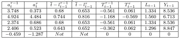
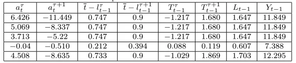
Main results are reported in tables 1-3. Tables 1.a, 2.a and 3.a report the matrix of inputs, whilst tables 1.b, 2.b and 3.b the matrix of outcomes. Tables 1.a and 1.b refer to periodt 1, tables 2.a and 2.b refer to periodt and table 3.a and 3.b refer to period t+ 1. We may notice some very interesting results. First of all, tax credits granted to the elder generation are sistematically higher than those granted to the younger generation. This happens at every period of time. Secondly, over time, there exists di¤erences in trends amongst generations. In fact, the trend of the old generation systematically increases over time, whilst the latter increases only from periodt 1to timet, and it dramatically decreases from periodt to time t+ 1. Hence, a …rst conclusion may be drawn: at time when debt is issued, both groups a reduction in the e¤ective marginal tax rate: the debt acts as a substitute of taxation. Otherwise, at time when the debt is paid o¤, we realize that the burden is borne only by the younger generation, whilst the older gets an even greater reduction in the e¤ective marginal tax rate. Another interesting result refers to the labour supply; we may note that the elder generation tends to work (rest) less (more) than the younger, with only one exception at timet+ 1 for simulations obtained with a nominal tax rate equal to 0.3 and 0.6. Nevertheless, notice that tax credits granted to the two groups are nearly the same. Furthermore, the labour supply increases over the three periods for both groups. As a consequence, also the total labour supply increases steadly over time. Tax revenues are always positive for the younger generation and always negative for the older generation, meaning that the former is a net taker, whilst the second is a net payer. Notice also that the tax bene…t for the older generation tends to increase over time and that tax revenues for the younger decreases when the debt is issued but dramatically increases once the debt must be repaid. This again underlies the asymmetry in the allocation of the burden: the young borne the cost of repayment. The last result refers to the level of production. For numerical simulations I used a production function equal toY = 10pL w 1_{(1 (1 a} 1 _{)(t l} 1_{) +w (1 (1 a )(t l ),}

whereL=t l 1_{+t l . It can be seen that at the period when the debt is}

5

I consider now a model where the old workers care of their o¤spring’s wealth. A classical altruistic model considers that households can be represented by a dinasty who is willing to perpetuate forever. As a consequence, the old inter-nalize the utility function of the young and thus the new utility function of the old may be written as:

U 1=ct 1+ 1

loglt 1+ U (23)

8 12T 1

where 2[0;1]is a parameter which captures the degree of altruism of the old for the young; the higher the more the old attach a greater importance to the young’s wealth. In Appendix 3 i will provide a complete resolution to the problem.

Proposition 5 The introduction of altruism in the model entails higher tax credits for the group of the young. The magnitude of this shift is higher, the higher is .

Proof: see Appendix 2. As we can see by numerical simulation reported in Appendix 3, the introduction of altruism turns previous results around. This time the group of the young gain higher tax credits than the group of the old which is higher the higher is the parameter representing altruism. Furthermore, the taxation on the old is positive whilst that on the young is negative, meaning that they get a …scal bene…t whose burden is carried by the old. Nevertheless, the old still reach higher level of leisure. Results are very easy to interpret: the higher the old care of the young’s welfare, the higher they are willing to accept to carry the burden of the social security system. This is a great achievement for the welfare of society: the old get satisfaction both from leisure and from being generous, whilst the young get satisfaction by working more and receiving a …scal bene…t; since Leviathan politicians want to satisfy the electorate, they are more than happy to set the new pro-younger policy.

6

7

8

In this Appendix I provide a complete resolution to the candidates’ problem. The two can-didates face exactly the same optimization problem; they maximize their share of votes or, equivalently, the probability of winning. The resolution is made for candidate A, but it also holds for candidate B.

max A= 1 2+

h s

X

I=fT 1;Tg

nIsI[Vi(q~A) Vi(~qB)]

T1 n 2 L(t lt 2)(1 at 2) +n 1 L(t lt 1)(1 at 1) = 0

at timet 1

T1bis n 1 L(t lt 1)(1 a

1

t ) +n L(t lt)(1 at) +Bt= 0

at timet

T1tris n L(t lt)(1 at) +n +1 L(t lt+1)(1 at+1) = (1 +r)Bt

at timet+ 1

I write the Lagrangian function for a given budget constraint BC:

`=1 2+

h s

X

I=fT 1;Tg

nIsI[Vi(~qA) Vi(~qB)] + (BC)

I obtain the following …rst order conditions which may be seen as a modi…ed version of the original Lindbeck and Weibull …rst order conditions, at timet:

(1) @L

@at 1

n 1@s 1

@lt 1

@lt 1

@at 1

(V 1A _V 1B_{) +n} 1_s 1₍@V 1

@at 1

) = @T(1)

@at 1

(2) @L @at n

@s @lt

@lt

@at(V

A _V B_{) +n s (}@V @at ) =

@T(1)

@at

(3)BC= 0

According to the result stated in Corollary 1, FOC’s can be re-written in the following man-ner:

(1) @L @at 1

n 1_s 1₍@V 1 @at 1

) = @T(1)

@at 1

(2) @L

@at n s (

@V @at ) =

@T(1)

@at

(3)BC= 0

and after some easy calculations, I obtain:

(1)n 1_s 1_(t

L+

1 _L

(1 (1 at 1) L)

) ((1 at 1) 2L 1n 1 (1 (1 at 1) L)2

) n 1

L(t

1

(1 (1 at 1) L) )) =

0

(2)n s (t L+_{(1 (1} aLt) L)) (

(1 at) 2L n

(1 (1 at) L)2 n L(t (1 (1 at) L))) = 0

From (1) and (2) obtain:

=

n 1_s 1_(t+ 1 (1 (1 at 1))

)

((1 at 1) L 1n 1 (1 (1 at 1) L)2

) n 1_(t 1

(1 (1 at 1) L) ))

=

n s (t+_{(1 (1 a} t))) ((1 at) L n

(1 (1 at) L)2 n (t (1 (1 at) L)))

Table 1.a- Main results obtained via numerical simulations withMathematica 5.2 - Input Matrix - Periodt-1

n 2 _n 1

L t 2 1 s 2 s 1 w ! r B

0:5 0:5 0:3 0:9 0:8 0:2 0:689 0:549 2 1 0:1 0:5 0:5 0:5 0:4 0:9 0:8 0:2 0:689 0:549 2 1 0:1 0:5 0:5 0:5 0:6 0:9 0:8 0:2 0:689 0:549 2 1 0:1 0:5 0:5 0:5 0:4 0:9 0:8 0:2 0:689 0:549 2 1 0:06 0:3 0:5 0:5 0:4 0:9 0:8 0:2 0:689 0:549 2 1 0:14 0:7

Table 1.b- Main results obtained via numerical simulations withMathematica 5.2 -Output Matrix - Periodt-1

at 2 at 1 t lt 12 t lt 11 Tt 12 Tt 11 Lt 1 Yt 1

Table 2.a- Main results obtained via numerical simulations withMathematica 5.2 - Input Matrix - Periodt

n 1 _n

L t 1 s 1 s w ! r B

0:5 0:5 0:3 0:9 0:8 0:2 0:689 0:549 2 1 0:1 0:5 0:5 0:5 0:4 0:9 0:8 0:2 0:689 0:549 2 1 0:1 0:5 0:5 0:5 0:6 0:9 0:8 0:2 0:689 0:549 2 1 0:1 0:5 0:5 0:5 0:4 0:9 0:8 0:2 0:689 0:549 2 1 0:06 0:3 0:5 0:5 0:4 0:9 0:8 0:2 0:689 0:549 2 1 0:14 0:7

Table 2.b- Main results obtained via numerical simulations withMathematica 5.2 -Output Matrix - Periodt

at 1 at t lt 11 t lt 1 Tt 11 Tt 1 Lt 1 Yt 1

3:748 0:373 0:68 0:653 0:561 0:061 1:334 8:536 4:924 4:484 0:744 0:816 1:168 0:569 1:560 6:713 2:374 0:686 0:68 0:653 0:561 0:061 1:334 8:536 2:406 0:523 0:643 0:652 0:362 0:062 1:296 8:847

Table 3.a- Main results obtained via numerical simulations withMathematica 5.2 - Input Matrix - Periodt+1

n n +1

L t +1 s s +1 w ! r B

0:5 0:5 0:3 0:9 0:8 0:2 0:689 0:549 2 1 0:1 0:5 0:5 0:5 0:4 0:9 0:8 0:2 0:689 0:549 2 1 0:1 0:5 0:5 0:5 0:6 0:9 0:8 0:2 0:689 0:549 2 1 0:1 0:5 0:5 0:5 0:4 0:9 0:8 0:2 0:689 0:549 2 1 0:06 0:3 0:5 0:5 0:4 0:9 0:8 0:2 0:689 0:549 2 1 0:14 0:7

Table 3.b- Main results obtained via numerical simulations withMathematica 5.2 -Output Matrix - Periodt+1

at at+1 t lt 1 t lt+11 Tt 1 Tt+11 Lt 1 Yt 1

References

[1] Barr, N.: Reforming pensions: Tales from China, Chile and elsewhere (2007), Barclay Memorial Lecture, London School of Economics

[2] Barr, N.: Pensions: Overview of the Issues(2006), Oxford Review of Economic Policy, Vol. 22 No. 1, pp. 1-14

[3] Barr, N. & Diamond, P:The Economics of Pensions(2006), Oxford Review of Economic Policy, Vol. 22 No. 1, pp. 15-39

[4] Barro, R.: Are Government Bonds Net Wealth (1974), Journal of Political Economy, Vol. 82 No. 6, pp. 1095-1117

[5] Barro, R.: On the Determination of the Public Debt (1979), Journal of Political Econ-omy, Vol. 87 No. 5, pp. 940-971

[6] : Boeri, T., Borsch-Supan, A., & Tabellini, G.: Would you like to shrink the welfare state? (2000), Economic Policy (32), pp. 7-50

[7] Brennan, G. & Buchanan, J.M:The Power to Tax: Analytical Foundations of a Fiscal Constitution, (1980) Cambridge: Cambridge University Press

[8] Buchanan, J. M.: Barro on the Ricardian equivalence theorem, (1976) Journal of Polit-ical Economy, Vol.84, pp.337–342

[9] Canegrati, E.: A Theory on the Allocation of Political Time (2007) mimeo

[10] Coile, C. & Gruber, J.: Social Security and Retirement, (2000) NBER Working Paper 7830

[11] Diamond P. & Mirrlees J. Optimal Taxation and Public Provision 1: Production E¢-ciency, (1971) American Economic Review, Vol.61, pp.8-27

[12] Diamond P. & Gruber J. Social Security and Retirement in the U.S., (1997) NBER Working Paper 6097

[13] Diamond P.Pensions for an Aging Population, (2005) NBER Working Papers 11877

[14] Diamond P.National Debt in a Neoclassical Growth Theory, (1965) American Economic Review, Vol.60, pp.1126-50

[15] Dixit, A. & Londregan J.Redistributive Politics and Economic E¢ciency, (1994) NBER Working Papers 1056

[16] Ferrera, M.: EC Citizens and Social Protection: Main Results from a Eurobarometer Survay, (1993), Brussels: European Commission, Division V/E/2.

[18] Feldstein, M.: Government de…cits and aggregate demand, (1982), Journal of Monetary Economics, Vol. 9, pp. 1–20.

[19] Feldstein, M.: The E¤ects of Fiscal Policies When Incomes Are Uncertain: A Contra-diction to Ricardian Equivalence, (1988), American Economic Review, Vol. 78(1), pp. 14-23.

[20] Feldstein M. & Liebman J.: Social Security, (2001) NBER Working Paper 8451

[21] Fuest C. & Huber B.: Tax Coordination and Unemployment, (1999) International Tax and Public Finance, Vol.6, pp.7-26

[22] Greenwood, J. & Vandenbroucke, G.: Hours Worked: Long-run Trends, (2005), NBER Working Paper 11629

[23] Gruber, J. & Wise, D.A.: Social Security and Retirement Around the World (1999), Chicago University Press

[24] Hershey D., Henkens K. & Van Dalen H.: Mapping the Minds of Retirement Planners: A Cross-cultural Perspective, (2006), mimeo

[25] Hinich M.J.: Equilibrium in Spatial Voting: The Median Voter Theorem is an Artifact, (1977) Journal of Economic Theory, Vol. 16, pp. 208-219

[26] Koskela E. & Schob R.: Optimal Factor Income Taxation in the Presence of Unemploy-ment, (2002) Journal of Public Economic Theory, Vol. 4(3), pp.387-404

[27] Kotliko¤, L. & Rapson, D:Comparing Average and Marginal Tax Rates under the Fair Tax and the Current System of Federal Taxation, (2006) Boston University, mimeo

[28] Ihori, T.: Public Finance in an Overlapping Generations Economy, (1996) MacMillan Press

[29] Ihori, T. & Tachibanaki, T.: Social Security Reforms in Advanced Countries, (2002) Routledge

[30] Lindbeck A. & Weibull J. W.: Balanced-Budget Redistribution as the Outcome of Po-litical Competition, (1987), Public Choice 52, pp. 273-297

[31] McCallum, B.: Are Bond-…nanced De…cits In‡ationary? A Ricardian Analysis, (1984), The Journal of Political Economy, Vol. 92(1), pp. 123-135.

[32] Mulligan C. B. & Sala-i-Martin: Gerontocracy, Retirement and Social Security, (1999) NBER Working Paper 7117

[33] Mulligan C. B. & Sala-i-Martin: Social Security in Theory and Practice (I): Facts and Political Theories, (1999) NBER Working Paper 7118

[35] Mulligan C. B. & Sala-i-Martin: Social Security, Retirement and the Single-Mindness of the Electorate, (1999) NBER Working Paper 9691

[36] O’Driscoll, G.P.: The Ricardian Nonequivalence Theorem, (1977) The Journal of Polit-ical Economy, Vol. 85, pp.207-210

[37] Profeta, P.: Retirement and Social Security in a Probabilistic Voting Model, (2002) International Tax and Public Finance, 9, pp 331-348

[38] Persson T. & Tabellini G.: Political Economics: Explaining the Economic Policy, (2000) MIT Press

[39] Ramsey F.P.: A Contribution to the Theory of Taxation, (1927) Economic Journal, Vol. 37, No. 1, pp. 47-61