http://dx.doi.org/10.4236/jcc.2016.42005
Effect of Transmission Range on Ad Hoc on
Demand Distance Vector Routing Protocol
Mohammad Izharul Hasan Ansari1, Surendra Pal Singh2, Mohammad Najmud Doja3 1Department of Computer Science & Engineering, NIMS University, Jaipur, India2Department of Computer Science & Engineering, NIMS University, Jaipur, India 3Department of Computer Engineering, JMI University, New Delhi, India
Received 16 January 2016; accepted 21 February 2016; published 24 February 2016
Copyright © 2016 by authors and Scientific Research Publishing Inc.
This work is licensed under the Creative Commons Attribution International License (CC BY). http://creativecommons.org/licenses/by/4.0/
Abstract
The necessary background as well as the details of simulation was presented to simulate and eva-luate the performance of the ad hoc on-demand distance vector routing protocol in mobile ad hoc network with the help of the network simulator NS2 using the common transmission range to de-liver the data packets at the destination node. The number of participating nodes played an im-portant role to predict the conditions for the best performance of the protocol with respect to throughput, delay, packet delivery ratio, drop packets, consumed and residual energy of the net-work. Further, the efforts can be put to control the transmission range dynamically and overheads for reducing the energy consumption in the network and improving its lifetime of the nodes and the lifespan of the network.
Keywords
MANET, Routing Protocol, Network Simulator, Transmission Range, Throughput, Delay, Packet Delivery Ratio, Energy Consumption, Efficiency and Lifetime
1. Introduction
one hand higher transmission powers cause an increase in the overheads during the transmission of data from one node to another, and on the other hand lower transmission powers adversely affect the participating mobile nodes by not allowing them to keep the network live for a longer duration thereby causing a loss of energy [1].
Over the last few years the various energy management schemes employing energy efficient routing protocols have been proposed in MANET to minimize the utilization of the battery power of the participating mobile nodes of the networks and extend the network lifetime [1] [2]. In this paper, we have analyzed such protocol, namely the Ad hoc On-Demand Distance Vector (ADOV) routing protocol to study the effect of the variable transmis-sion range on the various parameters, namely throughput, delay, packet delivery ratio (PDR), drop packets, consumed energy in transmitting data packets, and residual energy of the participating mobile nodes of the net-works. Our work is based on the simulation using Random Way Point Mobility Model [2]. We have investigated into the role of the required tramnsmision range from one node to another to minimize the energy consumption, which a study to the best of the authors’ knowledge has not been done much and reported in literature.
The paper is divided in seven sections including the present introductory section. In Section 2, we have revi-sited earlier work related to the present study. Section 3 is an overview on ADOV. In Section 4, we have pre-sented the various concepts related to the network simulators including NS2, while Section 5 is devoted to de-scribing the simulation setups, simulation environment, and mobility model, which have been subsequently used by us in our study of the evaluation of the performance of ADOV reported in Section 6. In Section 7 the work is concluded.
2. Related Work
In [3] is introduced the Minimum Energy Dynamic Source Routing (MEDSR) protocol for MANET in which the route discovery has been suggested both in low and high power levels. In this protocol, a higher power level is sought if three attempts of route request from one node to the next for the route discovery fail at a lower pow-er level. Howevpow-er, in MEDSR protocol, the enpow-ergy is conspow-erved and the ovpow-erall lifetime of the network is in-creased at the cost of the delay per data packet since the travel of data packets to the destination node involves a large number of hops. Thus, there is a scope for the improvement in the delay in this protocol.
Narayanaswamy et al. [4] proposed Common Power (COMPOW) control in MANET. It is based on the fol-lowing observation. Excessively high powers cannot be used to transmit the data packets from the source node to the destination node because of the shared medium, which also causes lot of interferences. This affects the traffic carrying capacity of the network and reduces the battery life. On the contrary if the network chooses low powers for establishing the routes then it leads to the route failure calling for the route maintenance and route discovery process to activate very frequently, which causes a loss of significant amount of energy. Therefore, the network power level must be chosen neither too high to cause excessive interference which results in a re-duced ability to carry traffic, nor too low to result in a disconnected network. The technique of COMPOW con-trol has been designed and tested only for table driven routing protocols and apart from this the technique is via-ble only for very dense network where the number of participating mobile nodes is very high and the covering area is small.
Hiremath and Joshi [5] proposed a fuzzy adaptive transmission range and fuzzy based threshold energy for the location aided routing protocol, namely Fuzzy Adaptive Transmission Range Based Power Aware Location Aided Routing (FTRPALAR). In this protocol proposed by them, the energy of a mobile node is conserved by employing a fuzzy adaptive transmission power control depending on the minimum number of neighboring nodes to maintain the network connectivity and power aware routing based on fuzzy threshold energy. Further, the experimental results on FTRPALAR obtained by them performs better in terms of the average energy con-sumption and network lifetime as compared to the conventional location aided routing (LAR) protocol and the variable transmission range power aware location aided routing (VTRPALAR) protocols. The proposed FTRPALAR is able to achieve 18% more lifetimes than VTRPALAR.
large numbers yet they consume significant amount of energy. This drawback of the MEDSR protocol is alle-viated in the HMEDSR protocol which is basically the combination of the protocols MEDSR and Hierarchical Dynamic Source Routing (HDSR), the latter reducing the overhead while the former saving energy in the trans-mission of data packets [6].
3. Overview of ADOV Routing Protocol
The ADOV protocol, which comes under the purview of reactive routing protocols, is of on-demand type in the sense that the route between two nodes is discovered only when it is needed. Such protocols are designed to make them least overburdened while they maintain the information only for those routes which are active [7]. It means that, in the process of route discovery and route maintenance, the routes are discovered and maintained only for the nodes that send their request to the specific destination. The various issues related to the ADOV protocol have been discussed in this section except the simulation parameters for analyzing the performance of ADOV which have been taken up separately in Section 5.
3.1. Route Discovery in AODV
The basic approach in the route discovery process is to establish the route in an on-demand routing protocol by broadcasting the route request message in the network. The destination node, on receiving a route request mes-sage, replies by sending a route reply message back to the source. The route reply message carries the route back to the source node that is traversed by the route request message received at the destination node [7]. In this process, when a particiapting node of a network wishes to send a data packet to some destination node then the source node checks its routing table to determine whether it has a current route to that destination node [7]. If the route is available with the destination node then it forward the pakcet to the appropriate next hop towards the destination node. However, if the particpating mobile node does not have a valid route to the destination node then the node must initiate the route discovery mechnism. Further, to begin this route discovery process, the node creats a RREQ packet and broadcast the route request packet at a low power level. Such a packet contains the source node IP address and current sequence number as well as the destinations IP address and the last known sequence number. The RREQ packet also contains a broadcast ID, which is increemented each time the source node initiate a RREQ. In this way, the broadcast ID and the IP address of the source node form a unique indetifier for the RREQ. After creating the RREQ, the source node broadcasts the packet and then sets a timer to wait for a reply. When a node receives a RREQ, it first checks wheather it has seen it before by noting the source IP address and the braodcast ID pair. Each node maintains a record of the source IP address/bradcast ID for each RREQ it receives, for a specified length of time. If it has already seen a RREQ with the same IP address/broadcast ID pair, it silently discards the packet. Otherwise, it records this information and then process the packet [7]. Further, in order to process the RREQ, the node sets up a reverse route entry for the source node in its route table. This reverse route entry contains the source nodes IP address and the sequence number as well as the number of hops to the source node and the IP addresses of the neighbor from which the RREQ was received. In this way, the node knows how to forward a RREP to the source if one received later [7]. Figure 1
indicates the propagation of RREQs across the network as well as the formation of the reverse route entries at each of the network nodes. Moreover, a lifetime is associated with the reverese route. If this route entry is not used within the specified lifetime, the route information is deleted to prevent the old routing information from lingering in the route table [7].
3.2. Propagation of Route Request
Figure 1. Propogation of route request (source: [7]).
mechnism. After RREQ-retries additional attempts, it is required to notify the application that the destination is unreachable [7] [8].
3.3. Forward Path Setup in AODV
When a route determines that it has an enough route current to respond to the RREQ, it creats a RREP [7]. For the purposes replying to a RREQ, any route with the sequence number not smaller than that indicated in the RREQ is deemed as asscociated with enough current. The RREP sent in response to the RREQ caontains the IP address of both the source and the destination. if the destination node is responding , it places its current sequence number in the packet, initilizes the hop count to zero, and then places the length of time of this route as valid in RREPs lifetime field. However, if an intermediate node is responding, it places its record of the destination’s sequence number in the packet, sets the hop count equal to its distance from the destination, and calculates the amount of time for which its route table entry for the destination will still be valid. It then unicasts the RREP towards the source node, using the node from which it receives the RREQ as the next hop [7] [8].
When the intermediate node receives the RREP, it sets a forward path entry to the destination in its route table. This forward path entry contains the IP address of the destination, the IP address of the neighbor from which the RREP had arrived, and the hop count, or the distance, to the destination. To obtain its distance to the destiantion, the node increaments the value in the hop count field by 1. Also associated with this entry is a lifetime, which is set to the lifetime contained in the RREP. Each time the route is used, its associated lifetime is updated. If the route is not used with in the specified lifetime, it is deleted. After processing the RREP, the node forwards it towards the source [7] [8]. Figure 2 indicates the path of the RREP from the destination to the source node.
3.4. Route Discovery from Source to Destination
Figure 2. Propogation of the route reply (source: [7]).
4. Simulation Details
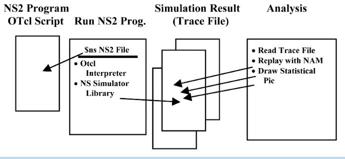
In this section we have decribed the network simulator NS-2, the execution process, the process to genrate the movement, the process of trafic genration, the mobility model as well as the simulation paramenters used in our simualtion.
The simulation technology as applied to the networking areas like network traffic simulation is relatively new [9]. The computer assisted simulation technologies can be applied in the simulation of networking algorithms or systems by using software engineering. The application field is smaller than that in general field of simulation and it could be natural that more specific and desirable requirements will be placed on network simulations in future [9]. For example, the network simulations can have more emphasis on the validity and performance of a distri-buted protocol or algorithm than on the visual or real-time visibility features of simulations. Moreover, one has to keep pace with the rapidly developing network technologies running on different software over the Internet with the involvement of many different organizations contributing to the whole process. That is why the network si-mulation always requires open platforms or software which should be scalable and enough to include different packages in the simulations of the whole network. Internet has also a main characteristic that it is structured with a uniformed network stack (TCP/IP) that has all the different layers of technologies which can be implemented in different ways while having uniform interfaces with their neighbored hops and layers [9] [10]. Thus, the network simulation tools must be able to incorporate these features and allow different future aspects and new packages to be included and run transparently without any harm to and with either no impact or at least no negative impact on the existing components or packages [9] [10]. Network simulators are mainly used by people from different backgrounds and areas like industrial developers, academic researchers and quality assurance (QA) for designing, simulating, verifying, and analyzing the performance of different networks protocols. Network simulators can also be used to evaluate and analyze the effect of the different parameters on the protocols being studied for network scenarios. Generally a network simulator will contain a wide range of networking protocols and technologies that help users to build complex networks from vary basic building blocks for example clusters of nodes and links. With the help of network simulators, one can design and propose different network topologies with the help of various types of nodes like end-hosts, hops, network bridges, routers, and mobile units [10]. The present section is thus of relevance to the simulation based study taken up in this paper on AODV to know effect of the variable transmission range on it as mentioned in Section 1.
4.1. Network Simulator NS-2
and wireless networks [9]. Initially, it was designed and developed for the simulation of wired technology only but later the Monarch Group of the department of computer science at the University of Rice developed the ne-cessary tools and applications to include in the simulator for the wireless and mobile hosts [9]. In NS-2, the si-mulations are written in C++ with an OTcl API (seeFigure 3).
The user creates a text file in OTcl which describes the layout of the whole network as well as the events to be occurred such as transferring data or node movement application. This OTcl file (.tcl) is executed and a detailed trace file (.tr) is generated which can be filtered with a pattern matching program (such as “grep” or “awk”) and inspected by hand, or fed into a visualization tool [9]. Some visualization tools are also available with NS-2, one of which is the Network Animator (NAM). NAM is an animation tool for viewing network simulation traces in graphical form. It supports topology layout and has various data inspection tools. NS-2 is suitable for simulating MANET because it has accurate implementations of the IEEE 802.11 standard, a TCP/IP stack and a wide range of routing protocols implemented for NS-2 [9].
4.2. Node Movement Generation for Wireless Scenarios in NS-2
We can define the node movement in separate files called as scenario file in NS with the help of node movement generation tool available in NS-2. This scenario file is generated with help of this tool which is available on the “ns-2/indep-utils/cmu-scen-gen/setdest/” location. This scenario file is used to store the information about the initial position of the nodes with their movement details, speed, etc. at various points of time. Generally, since it is very difficult to provide the initial position of the participating mobile nodes manually, movement of the nodes and their speed for each movement at different times we use a random file generator. We can run this tool with following command [9]:
./setdest –n [num of nodes] –p [pause time] –m[max speed] –t[sim time] –x[max x] –y[max y]>[outdir/movement file],
for example:
./setdest -n 20 –p 0.0 -m 2.0 -t 200 -x 1000 -y 1000 > scen-20-test
Here, the number of nodes n is: n = 20, the pause time p is p = 0.0 s, maximum speed m is m = 2.0 m/s, simu-lation time t is t = 200 s, and area x × y is equals to 1000 × 1000, and scen-20-test is the desired scenario file.
4.3. Random Traffic Generation for Wireless Scenarios in NS-2
In NS-2 we can set up random traffic connections between mobile nodes of TCP and CBR using traffic-scenario generator script. This script is available at ~ns/indep-utils/cmu-scen-gen location and is called cbrgen.tcl. It is used to generate CBR and TCP traffics connections between mobile nodes. For this purpose we create a traf-fic-connection file, in which we need to define different parameters like the type of traffic connection (CBR or TCP), maximum number of connections to be set up between the nodes, the number of nodes and a random seed and, for CBR connections, a rate. The inverse value of the rate is to compute the interval time between the pack-ets [9]. We can generate this with the following command:
[image:6.595.143.487.551.710.2]ns cbrgen.tcl [-type cbr/tcp] [-nn nodes] [-seed seed] [-mc connections] [-rate rate] > [outdir/movement file]
The start times for the connections are generated randomly with a maximum value of 180.0 s. For example, we can have a CBR connection file with 10 nodes, having maximum of 8 connections, seed value of 1.0 and a rate of 4.0. So we can do this with following command:
ns cbrgen.tcl -type cbr -nn 10 -seed 1.0 -mc 8 -rate 4.0 > cbr-10-test This generates a random traffic pattern with described values.
4.4. Tool Command Language (Tcl)
There are two languages used in NS2 C++ and OTcl (an object oriented extension of Tcl) [9]. The compiled C++ programming hierarchy makes the simulation efficient and execution times faster. The simulation results produced after running the scripts can be used either for simulation analysis or as an input to NAM.
Tool Command Language Tcl is a powerful interpreted programming language developed by John Ouster out at the University of California, Berkeley [9]. Tcl is a very powerful and dynamic programming language. Tcl is a truly cross platform, easily deployed and highly extensible. The most significant advantage of Tcl language is that it is fully compatible with the C programming language and Tcl libraries can be interoperated directly into C programs.
4.5. NAM
NAM for the graphical representation of the simulation have been designed and developed in 1990 as a simple tool for animating packet trace data [9]. This trace data is typically derived as the output from a network simu-lator like NS or from real network measurements, e.g., using tcpdump. Steven McCanne wrote the original ver-sion as a member of the Network Research Group at the Lawrence Berkeley National Laboratory, and has occa-sionally improved the design [9]. Marylou Orayani improved it further and used it for her Master's research over summer 1995 and into spring 1996 [9]. The NAM development effort was an ongoing collaboration with the Virtual Internetwork Test bed (VINT) project. Currently, it is being developed at ISI by the Simulation Aug-mented by Measurement and Analysis for Networks (SAMAN) and Conser projects [9].
4.6. Trace File
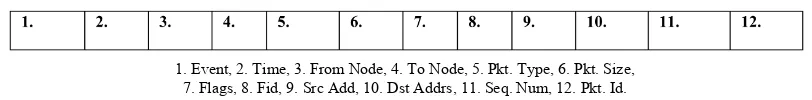
The trace file is an ASCII code files and the trace is organized in 12 fields as inFigure 4.
The first field is the event type and given by one of four available symbols r, +, − and d which correspond re-spectively to receive, en-queued, de-queued and dropped. The second field is telling the time at which the event occurs. The third and fourth fields are the input and output nodes of the link at which the events takes place. The fifth is the packet type such as Constant Bit Rate (CBR) or Transmission Control Protocol (TCP). The sixth is the size of the packet and the seventh is some kind of flags. The eighth field is the flow identities of IPv6, which can specify stream color of the NAM display and can be used for further analysis purposes. The ninth and tenth fields are respectively the source and destination address in the form of “node.port”. The eleventh is the network layer protocol’s packet sequence number. NS keeps track of UDP packet sequence number for the analysis pur-poses. The twelfth, which is the last field, is the unique identity of the packet. Results of simulation are stored into trace file (*.tr). Trace Graph was used to analyze the trace file.
5. Simulation Setup
Let us now consider the simulation setup as relevant to the ultimate goal of our research work which is to eva-luate the dependence of AODV on the various parameters and then develop a new technique for the optimum utilization of transmission power for transmitting the data packet from the source to the destination node suc-cessfully and in timely manner so as to increase the lifetime of the battery of the participating mobile nodes and that of the network as a whole. The five parameters which we have chosen for our studies are: 1) the density of
[image:7.595.110.516.656.706.2]1. Event, 2. Time, 3. From Node, 4. To Node, 5. Pkt. Type, 6. Pkt. Size, 7. Flags, 8. Fid, 9. Src Add, 10. Dst Addrs, 11. Seq. Num, 12. Pkt. Id.
Network; 2) the speed of participating mobile nodes; 3) the transmission power of the participating mobile nodes and 4) the data traffic pattern. In the simulation the participating mobile nodes move according to a model called Random Waypoint which was proposed by Johnson and Maltz [11]. Now, this mobility model is widely being used because of its simplicity and wide availability. To generate the node trace of the Random Waypoint model the setdest tool from the CMU Monarch group may be used. This tool is included in the widely used network simulator NS-2 [11].
In NS-2 distribution, every participating mobile node randomly selects one location in the simulation field as the destination. The participating nodes then move towards the destination with constant velocity chosen un-iformly and randomly from (0, V), where the parameter Vmax is the maximum allowable velocity for every par-ticipating mobile node of the networks [12]. After reaching the destination, the node stops for a duration defined by the pause time. If pause time Tpause = 0 then the participating mobile does not stop and keeps itself moving continuously. After this pause time, it once again chooses another random destination in the simulation field and moves towards it. The same process is repeated again and again until the simulation ends.
In the Random Waypoint mobility model, V and T are the two key parameters that determine the mobility behavior of nodes. If V is small and T is long, the topology of ad hoc network becomes relatively stable. On the other hand, if the node moves fast (i.e., Vmax is large) and T is small, the topology is expected to be highly dy-namic. Varying these two parameters, especially the V parameter, the Random Waypoint model can generate various mobility scenarios with different levels of nodal speed. Therefore, it seems necessary to quantify the nodal speed. Intuitively, one such motion is the average node speed. If we could assume that the pause time Tpause = 0 max, considering that Vmax is uniformly and randomly chosen from (0, V), we can easily find that the average nodal speed is 5.0 m/s [13] [14]. However, in general, the pause time parameter should not be ignored. In addition, it is the relative speed of two nodes that determines whether the link between them breaks or forms, rather than their individual speeds. Thus, the average node speed seems not to be the appropriate metric to represent the notion of the nodal speed.
5.1. Mobility Model
During simulation each node starts moving from its initial position to a random direction with random speed. The speed is uniformly distributed between 0 and the maximum speed. When a moving node reaches the boun-dary of the given area, it waits for the pause time (which is 0 in our case) and after that once again starts to move in a random direction and with random speed. The entire traffic source used in our simulation generated Con-stant Bit Rate (CBR) data traffic. The traffic structure was defined by varying two factors: 1) the sending rate and 2) the packet size.
5.1.1. Simulation Environment
As the basic scenario we considered a MANET with 10, 20, 30, 40 and 50 mobile nodes spread randomly over an area of 1000 m by 1000 m. The nodes were moving with a maximum speed of 2 m/sec with pause time of 0 sec. A total of 01 traffic sources generated CBR data traffic with a sending rate of 4 packets/sec, using a packet size of 512 bytes.
Each simulation had the duration of 500 simulated seconds. Because the performance of the simulations is highly related with the mobility models, the result to be shown in Section 6 represents an average of three dif-ferent executions of the simulation using the same traffic models but with difdif-ferent randomly generated mobility scenarios (Table 1).
We evaluate the following performance indexes: 1) total energy consumed (in Joules); 2) energy consumed depending on the operation (Transmissions (Tx) and Receptions (Rx)) and 3) energy consumed depending on the packet type (MAC, CBR and routing).
6. Result and Discussion
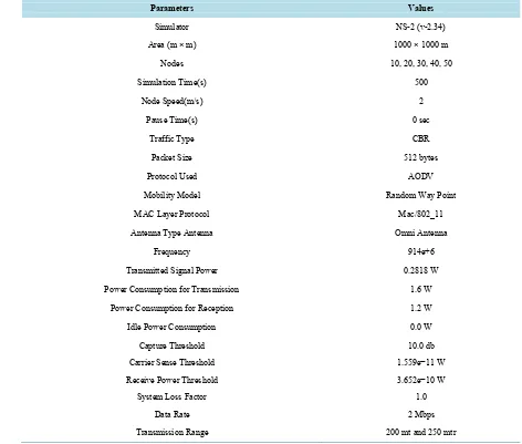
Table 1. Simulation parameter.
Parameters Values
Simulator NS-2 (v-2.34)
Area (m × m) 1000 × 1000 m
Nodes 10, 20, 30, 40, 50
Simulation Time(s) 500
Node Speed(m/s) 2
Pause Time(s) 0 sec
Traffic Type CBR
Packet Size 512 bytes
Protocol Used AODV
Mobility Model Random Way Point
MAC Layer Protocol Mac/802_11
Antenna Type Antenna Omni Antenna
Frequency 914e+6
Transmitted Signal Power 0.2818 W
Power Consumption for Transmission 1.6 W
Power Consumption for Reception 1.2 W
Idle Power Consumption 0.0 W
Capture Threshold 10.0 db
Carrier Sense Threshold 1.559e−11 W
Receive Power Threshold 3.652e−10 W
System Loss Factor 1.0
Data Rate 2 Mbps
Transmission Range 200 mt and 250 mtr
calculated for this scenario. The diffeerent scenarios have been created after increasing the density of the particiapting mobile nodes in the networks for anlyzing the performance of the AODV routing protocol in MANET.
6.1. Throughput versus Transmission Range
The throughput for node 10 is found to be the least in the throughput versus transmission range characteristics (Figure 5).
Further, as we increase the density of the particiapting mobile nodes in the networks without changing the area of the netwrok, the throughput increases with the increase of the transmission range (Figure 5: Throughput versus transmission range) owing to the high desity of the participating mobile nodes in the nework. Because of the dense nework most of the particiapting mobile nodes are nearer and within the transmission range of each other and the route faliures and route maitenenace are very less and the throughput is very high.
6.2. Delay versus Transmission Range
Figure 5. Throughput versus transmission range.
is much higher compared to the other scenarios, which decreases gradually, as the node density and the transmisison range are increased within the same network area (Figure 6).
Further, the delay is the least for 30 nodes showing the consistancy (Figure 6). However, in case of 50 nodes in the same geographical area at some points the delay is found to be higher as compared to the node denisties of 30 and 40 while it is lesser as compared to the node denisties of 10 and 20 (Figure 6). Thus, one has to choose an optimum value of the number of nodes to minimize the delay. As we increases the node density and as well as the transmission power of the participating mobile nodes, the distance between the participating nodes decreases becoming closer to each other and also within the tranimission range of each other (Figure 6). Due to high density of the network, the overhearing increases among the participating mobile nodes and the overheads and congetion increase by many folds, which adversly affects the bandwidth utilization as well as the congetion-free routes to transmit the data from one node to another in the networks. Because of this, the delay increases during the transmission of the data among the participating mobile nodes of the networks.
6.3. Packet Delivery Ratio versus Transmission Range
Various scenarios for the networks have been generated to evalute the performance of the participating mobile nodes and networks in terms of the packet delivery ratio (PDR)defined as the as the ratio of the number of the data packets delivered at the destination to those generated by the source nodewith respect to the tranimission ranage. In Figure 7 the increase in PDR with the increase in the number of modes can be seen.
However, beyond a threshold number of modes, no further increase in PDR is realized (Figure 7). Further, there is the least PDR when the desity of the participating mobile nodes is the least and packet delivery ratioincreases with the density of the particiapting mobile nodes in the networks (Figure 7). The overheads increase in the networks with the increase of the density of the networks and because of the nodes coming closer to each other. This affects adeversly the networks in terms of the throughput and delay. However, the PDR is affected to a lesser extent increasing only up to a little extent unless the density of nodes is increased to a larger extent, the terrain remaining the same, when the PDR also gets adversely affected. Here, in the given scenario the speed of the participating mobile nodes is constant and is very less because of the less speed the PDR increases with the incraeses of density and tranismission range of the participating mobile nodes of the networks.
6.4. Drop Packet versus Transmission Range
The drop packets are found to increase with the decease in the density of the participating mobile nodes with respect to the tranismission range (Figure 8). Further, with the increase in the transmission range of the participating mobile nodes the number of the drop packets increases (Figure 8).
Furthermore, the number of drop packets is found to be the least when the density of the paticipating mobile nodes is 30. However, in the same scenario of node 30, the drop packets increase with the increase in the the transmission range (Figure 8) attributable to the congestion due to overhearing.
Figure 6. Delay versus transmission range.
Figure 7. Packet delivery versus transmission range.
Figure 8. Drop packet versus transmission range.
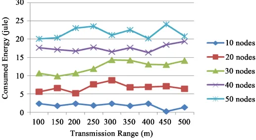
6.5. Consumed Energy versus Transmission Range
The energy consunption increases with the increase in the number of nodes (Figure 9). Thus, we can increase the packet delivery ratio and decrease the numbers of drop pakcets if we increases the transmission power of the particpating mobile nodes but at the cost of high energy consumption. Because of very high energy consumtions the lifespan of the networks is very short and it may be possilble that the participating mobile nodes could not actively particiapte in the transimission of the data packets from the source node to the destination node.
Due consideration needs to be given in choosing the number of participating mobile nodes in the network and the transmision power since, when these quantities are very less, the energy consumption to tranmit the data packet from the source node to the destination node becomes very less (Figure 9).
6.6. Residual Energy versus Transmission Range
[image:11.595.188.442.404.535.2]network increases because we found that the amount of the resedual energy of the of the network is higher, i.e., the lifetime of the whole netwok increases and more data can be trasnfered from one node to another (Figure 10). However, if we increase the number of nodes in the network as well as the transmission range of the particiapting mobile nodes then the lifetime of the particiapting mobile nodes gets aderversly affected remembering that the overheads inscrease beacause of high density and transmission range of the particiapting mobile nodes (Figure 10). This also means that a very high amount of energy is consumed by the particiapting mobile nodes and less residual energy is left for transmitting the data packet in the network which adeversly affects the lifetime of the particiapting mobile nodes and hence also that of the network as a whole.
7. Conclusion
[image:12.595.182.441.392.534.2]We have by simulation investigated into the effect of varying the transmission range on the throughput, delay, packet delivery ratio, drop packets, consumed and residual energy of ADOV routing protocol in MANET taking the number of particiapting nodes as the parameter. All the necessry background and details of simulation have been provided. The study shows that one can achieve higher values of throughput by increasing the number of particiapting nodes. However, due care should be taken to optimize the mumber of the particiapting nodes to minimize the delay while also noting that a larger value of delay is caused by overhearing congestion. Further, the PDR can be increased and the drop packets, which increase with the increase in the transmission range, can be decreased by increasing the number of nodes. One has to compromise on the energy consumption, which increases with the increase in the number of nodes, to get the best performance in terms of throughput, delay, PDR and drop packets. This is because sufficient amount of energy is consumed and less resudual energy left to the participating mobile nodes to transmit the data pakets from the source to destination node successfully, thereby adversely affecting the lifetime of the particiapting mobile nodes and also the lifespan of the whole networks. Further, there is scope to control the transmission range dynamically and reduce the overheads for reducing the energy consuption.
[image:12.595.179.456.555.705.2]Figure 9. Consumed energy versus transmission range.
Acknowledgements
Helpful criticism from Professor B N Basu and constant inspiration from Vice-Chancellor Dr. R M Dubey are gratefully acknowledged.
References
[1] Chlamtac, I., Conti, M. and Liu, J.J.-N. (2003) Mobile Ad Hoc Networking: Imperatives and Challenges. Ad Hoc Net-works, 1, 13-64. http://dx.doi.org/10.1016/S1570-8705(03)00013-1
[2] Bouallegu, M., Raoof, K., Zid, M.B. and Bouallegue, R. (2014) Impact of Variable Transmission Power on Routing Protocols in Wireless Sensor Networks Wireless Communications. 10th International Conference on Networking and Mobile Computing (WiCOM 2014), 26-28, 496-499. http://dx.doi.org/10.1049/ic.2014.0152
[3] Tarique, M. and Islam, R. (2007) Minimum Energy Dynamic Source Routing Protocols for Mobile Ad Hoc Networks.
International Journal of Computer Science and Network Security, 7, 304-311.
[4] Narayanaswamy, S., Kawadia, V., Sreenivas, R.S. and Kumar, P.R. (2002) The COMPOW Protocol for Power Control in Ad Hoc Networks: Theory, Architecture, Algorithm, Implementation and Experimentation. Proceedings of Euro-pean Wireless Conference, Florence, 25-28 February 2002, 1-20. http://citeseerx.ist.psu.edu
[5] Hiremath, P.S. and Joshi, S. (2014) Fuzzy Adaptive Transmission Range Based Power Aware Location Aided Routing.
International Conference on Information and Communication Technologies, Shivamogga, 5-6 May 2014, 296-301. [6] Tarique, M. and Tape, K.E. (2009) Minimum Energy Hierarchical Dynamic Source Routing for Mobile Ad Hoc
Net-works. Ad Hoc Networks, 7, 1125-1135. http://dx.doi.org/10.1016/j.adhoc.2008.10.002
[7] Perkins, C.E. and Royer, E.M. (2004) The Ad Hoc On-Demand Distance-Vector Protocol, Ad Hoc Networking. 2nd Edition, Ad Hoc Networking, Addison-Wesley, NJ, 173-219.
[8] Murthy, C.S.R. and Manoj, B.S. (2004) Routing Protocols for Ad Hoc Wireless Networks, Ad Hoc Wireless Networks —Architectures and Protocols, Prentice Hall Communications Engineering and Emerging Technologies Series. 2nd Edition, Prentice Hall, Upper Saddle River, 299-359.
[9] The NS Manual (Formerly NS Notes and Documentation) (2011) The VINT Project: A Collaboration between Re-searchers at UC Berkeley, LBL, USC/ISI, and Xerox PARC. 5 November.
[10] Francisco, J. and Ruiz, R.P.M. (2004) A Manual on Implementing a New Manet Unicast Routing Protocol in NS2. Department of Information and Communications Engineering University of Murcia December.
[11] Broch, J., Maltz, D.A., Johnson, D.B., Hu, Y.-C. and Jetcheva, J. (1998) A Performance Comparison of Multi-Hop Wireless Ad Hoc Network Routing Protocols. Proceedings of the 4th Annual ACM/IEEE International Conference on Mobile Computing and Networking (MobiCom’98), October 1998, 85-97.
[12] Breslau, L., Estrin, D., Fall, K., Floyd, S., Heidemann, J., Helmy, A., Huang, P., McCanne, S., Varadhan, K., Xu, Y. and Yu, H. (2000) Advances in Network Simulation (NS). IEEE Computer, 33, 59-67.
http://dx.doi.org/10.1109/2.841785
[13] Johansson, P., Larsson, T., Hedman, N., Mielczarek, B. and Degermark, M. (1999) Scenario-Based Performance Analysis of Routing Protocols for Mobile Ad-Hoc Networks. International Conference on Mobile Computing and Networking (MobiCom’99), New York, 17-19 August 1999, 195-206. http://dx.doi.org/10.1145/313451.313535 [14] Bettstetter, C., Hartenstein, H. and Perez-Costa, X. (2004) Stochastic Properties of the Random Waypoint Mobility
![Figure 1. Propogation of route request (source: [7]).](https://thumb-us.123doks.com/thumbv2/123dok_us/7999095.761110/4.595.173.447.87.346/figure-propogation-route-request-source.webp)
![Figure 2. Propogation of the route reply (source: [7]).](https://thumb-us.123doks.com/thumbv2/123dok_us/7999095.761110/5.595.189.461.94.283/figure-propogation-route-reply-source.webp)