http://dx.doi.org/10.4236/abb.2016.72010
How to cite this paper:
Uchino, T., Nakamura, Y., Sekino, M., Kai, W., Fujiwara, A., Yasuike, M., Sugaya, T., Fukuda, H., Sano,
M. and Sakamoto, T. (2016) Constructing Genetic Linkage Maps Using the Whole Genome Sequence of Pacific Bluefin Tuna
(
Thunnus
orientalis
) and a Comparison of Chromosome Structure among Teleost Species.
Advances
in
Bioscience
and
Bio-technology
,
7
, 85-122.
http://dx.doi.org/10.4236/abb.2016.72010
Constructing Genetic Linkage Maps Using
the Whole Genome Sequence of Pacific
Bluefin Tuna (
Thunnus
orientalis
) and a
Comparison of Chromosome Structure
among Teleost Species
Tsubasa Uchino
1, Yoji Nakamura
2, Masashi Sekino
2, Wataru Kai
2, Atushi Fujiwara
2,
Motoshige Yasuike
2, Takuma Sugaya
3, Himeko Fukuda
1, Motohiko Sano
1,
Takashi Sakamoto
1*1
Faculty of Marine Science, Tokyo University of Marine Science and Technology, Tokyo, Japan
2
Research Center for Aquatic Genomics, National Research Institute of Fisheries Science, Fisheries Research
Agency, Yokohama, Japan
3
Research Center for Marine Invertebrate Animals, National Research Institute of Fisheries and Environment of
Inland Sea, Fisheries Research Agency, Hiroshima, Japan
Received 15 January 2016; accepted 21 February 2016; published 24 February 2016
Copyright © 2016 by authors and Scientific Research Publishing Inc.
This work is licensed under the Creative Commons Attribution International License (CC BY).
http://creativecommons.org/licenses/by/4.0/
Abstract
Pacific bluefin tuna (
Thunnus
orientalis
) is one of the most economically important species in the
Percomorpha group of teleost fishes. Their migrations are extensive and depend upon continuous
swimming at a high rate of speed throughout their life. The draft genome sequence of this species
has been reported but remains highly fragmented. We constructed a Pacific bluefin tuna genetic
linkage map using microsatellite markers developed on each of the scaffolds from the draft
ge-nome sequence to link these gege-nome fragments and understand the genomic structure of species
in Percomorpha. Of the 606 polymerase chain reaction microsatellite primer pairs tested, 473
were polymorphic in the mapping populations for the linkage analysis. We constructed sex-spe-
cific maps for 24 linkage groups consisting of 470 markers, which allowed us to place scaffolds
that cumulatively represented 20.8% (153.8 Mb) of the sequenced genome onto the linkage
groups. The distribution of orthologous genes on the chromosomes of tuna and four other teleost
fish species suggested that the constitution of tuna chromosomes is closest to that of medaka. Both
species have the 24 chromosomes of the ancestral teleost, including several chromosomal
inver-*
sions. The integrated map developed in this study will be useful to construct a complete physical
map to conduct comparative teleost genomics and genetic studies on economically useful traits in
Pacific bluefin tuna.
Keywords
Pacific Bluefin Tuna, Microsatellite Marker, Genetic Linkage Map
1. Introduction
Pacific bluefin tuna (
Thunnus
orientalis
) is one of the most economically important species of fish, and their
migrations are unique, as they swim quickly and continuously throughout their life. This continuous swimming
ability enables Pacific bluefin tuna to migrate long distances in the Pacific Ocean. Continual swimming is
re-quired, so that water containing oxygen flows continuously over the gills; this is a special feature of
Thunnus
and closely related species. Tuna have superior swimming ability due to a large quantity of red muscle, a rapid
metabolic rate, large body size, and their unique shape and swimming form, although details remain unknown.
Moreover, the tuna growth rate is very high, as they can grow 50 cm in total length in 1 year. Maximum length
and weight are about 2.5 m and 300 kg, respectively. These unique ecological features of Pacific bluefin tuna
originate from their genome.
Tuna farmers generally use natural seed for broodstock. However, tuna catch is restricted by international
fishing regulations created as a result of recent decreases in wild population numbers
[1]
. Thus, a breeding
sys-tem that depends on the recruitment of naturally occurring siblings is difficult to maintain. The complete
life-cycle has been established recently for Pacific bluefin tuna aquaculture
[2]
and artificial seed is now being used
for production. Therefore, there is much interest in creating broodstock with commercially valuable genetic
traits.
Several whole genome sequences have been reported recently in teleosts because of the development of
high-throughput sequencing methods. Whole genome sequences have been registered in public databases for
model fish, such as zebrafish (
Danio
rerio
)
[3]
and medaka (
Oryzias
latipes
)
[4]
as well as for other fish, such as
fugu (
Takifugu
rubripes
)
[5]
,
Tetraodon
(
Tetraodon
nigroviridis
)
[6]
, stickleback (
Gasterosteus
aculeatus
)
[7]
,
and Pacific bluefin tuna
[8]
.
The draft Pacific bluefin tuna genome sequence was generated using the Roche 454 FLX Titanium and
Illu-mina GaIIx next-generation sequencing platforms
[8]
. Whole genome shotgun sequencing and assembly
pro-vided 192,169 contigs (>500 bp) and 16,802 scaffolds (>2 kb). The N50 values, which are used to evaluate
connectivity of the assembly, are 7588 bp (contigs) and 136,950 bp (scaffolds), respectively.
Cytological studies
[9] [10]
have reported that
Thunnus
species have 24 pairs of chromosomes. Draft genome
sequence when merged should, therefore, only have 24 huge fragments corresponding to each chromosome. The
draft genome sequence of this species is highly fragmented, and constructing a genetic linkage map is an
effec-tive way to link the sequence fragments. Genetic linkage maps have been used as an anchor for fish
[11] [12]
,
plants
[13]-[16]
, and domestic animals
[17]
. A genetic linkage map is constructed by developing genetic
mark-ers on scaffolds and examining the linkage relationships between the markmark-ers. However, no genetic linkage map
has been constructed for Pacific bluefin tuna. Several different classes of polymorphic markers could be used to
construct genetic linkage maps. Repetitive sequence regions called microsatellites (MS) (or short tandem repeats)
are abundant in eukaryotic genomes and have the potential to exhibit high polymorphism in a mapping
popula-tion. MS markers also have the benefit of being multi-allelic within species, and therefore, unlike single
nucleo-tide polymorphism markers (SNPs), MS markers can be used to track the unique segregation phases of both
male- and female-specific parental alleles in their progeny. When parents are doubly heterozygous for SNP
markers, the linkage phase of heterozygous progeny cannot be assessed. Only a few MS markers have been
de-veloped for Pacific bluefin tuna
[18]
, and therefore, there is a need to develop additional markers for this
spe-cies.
Recently, four novel candidates for vertebrate SD genes were reported, all of them in fishes. These include
trout
[22]
. There are multiple sex-determining regions in teleost fishes that do not possess homology to one
another due to the turnover of sex chromosomes
[23]
. In bluefin tuna the sex-determining region has been
iden-tified to by XY based, and male-specific marker (
male
delta
6 or
Md
6) has been characterized
[24]
. There is no
syntenic information about
Md
6 and those sex-determining regions in teleost fishes. One of the objectives of this
study was to localize the sex-determining locus within the genomic scaffolds corresponding to the genetic
lin-kage map placements by mapping
Md
6 using an adjacent MS marker.
Comparative genome studies have revealed the evolution of chromosomes among several fish species. These
studies suggest that the medaka genome has the conserved genomic structure of the MTZ ancestor (the last
common ancestor of three fishes, medaka,
Tetraodon
, and zebrafish) and no major chromosomal rearrangements
have occurred for more than 300 million years (My)
[4] [25]
, whereas the zebrafish genome has experienced
many interchromosomal rearrangements during evolution due to extensive translocations. A comparative
ge-nome study of fugu supported their hypothesis and discussed inter-chromosomal rearrangements in the fugu and
Tetraodon
lineages
[12]
. Tongue sole also experienced three major chromosomal fusion events after divergence
from the common ancestor with medaka,
Tetraodon
, and fugu
[26]
. A high density genetic map with tiled
ge-nomic platyfish contigs revealed that the platyfish and medaka karyotypes are remarkably similar with few
in-terchromosomal translocations but with numerous intrachromosomal rearrangements (transpositions and
inver-sions) since their lineages diverged about 120 Mya
[27]
. That study also suggested that stickleback and
Tetrao-don
arose by fusion of pairs of ancestral chromosomes. These results suggest that the chromosomal constitution
and synteny of fish in Percomorpha are highly conserved, with few inter-chromosomal rearrangements despite
substantial phylogenetic distances among the taxa compared
[28] [29]
. Percomorpha is a large group in
Acan-thopterygii that includes medaka, platyfish, fugu,
Tetraodon
, stickleback, tongue sole, European seabass, and
Pacific bluefin tuna. Accordingly, constructing a genetic map for other non-model fish species in Percomorpha
using gene information on scaffolds from whole genome sequences will provide new aspects for comparative
studies in this group.
The aim of the present study was to construct a genetic linkage map for Pacific bluefin tuna based on draft
genome sequence information to understand the genome structure of this species in Percomorpha. We extracted
an F1 full-sib population of young Pacific bluefin tuna as a mapping population. We constructed a linkage map
using MS markers developed on each of the scaffolds and examined preservation of chromosome structure in
four other fully sequenced fish species.
2. Materials and Methods
2.1. Mapping Population
Many full-sib progeny and their parents were prepared to construct a linkage map for the mapping population.
Unlike other fish that spawn easily, one-to-one mating is very difficult in Pacific bluefin tuna. Thus, we tried to
extract full-sib progeny from young fish spawned naturally from several parents. We collected 500 progeny (18
days old) derived from a small number of parents based on our visual observations at Amami Station, Seikai
National Fisheries Research Institute, FRA. The parents of these young fish were derived from wild fish
cap-tured offshore of Shimane in the Japan Sea and reared 3 years at Amami Station, Seikai National Fisheries
Re-search Institute, FRA. The whole bodies of the small fish were preserved in 100% ethanol until extraction of
genomic DNA. DNA extraction was conducted using the Quickgene system (Fujifilm, Tokyo, Japan), following
the manufacturer’s protocol. Candidate adult parents of these progeny were treated using the same method,
ex-cept a fin clip was collected as the sample. Genomic DNA was amplified using the Illustra GenomiPhi
Amplifi-cation Kit (GE Healthcare, Milwaukee, WI, USA) following the manufacturer’s protocol. A parental analysis of
500 young individuals was performed using 11 MS loci to select the full-sib progeny. Parent-offspring
hypo-theses were examined based on genotypic incompatibilities between putative parents and offspring using the
ex-clusion method. The parentage assignment test in PARFEX software
[30]
was used with the exclusion method.
We allowed for a few genotype mismatches (<2) between offspring and parents per MS marker due to missing
data or the influence of a null allele.
2.2. Development of Microsatellite Markers
1.98 Kbp
[8]
. The positional information of longer scaffolds was revealed using linkage analysis during
con-struction of the tuna physical map. Therefore, we selected the longest 1000 scaffolds as mapping candidates.
Primer 3
[31]
was used to design the appropriate polymerase chain reaction (PCR) primers for the near-detected
MS regions that had repeat units ranging from two to five nucleotides. The size of the amplified PCR product
was set to 100 - 400 bp in the reference sequence. We selected one PCR primer pairs from each scaffold, and
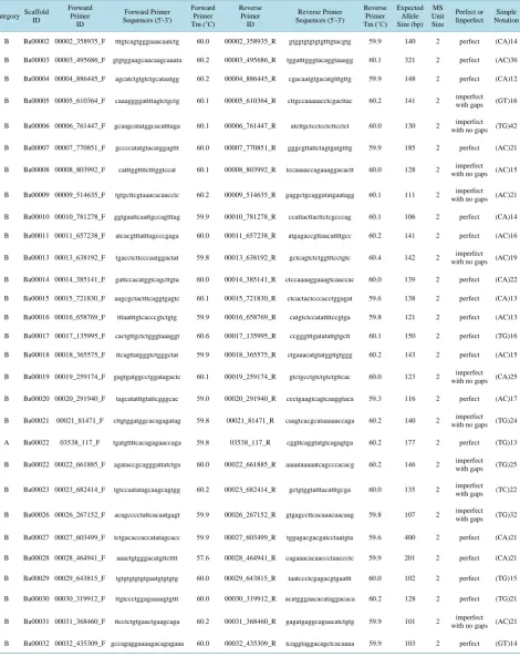
606 PCR primer pairs for MS were tested for polymorphism in the mapping population (
Supplementary Table
S1
).
2.3. Genotyping and Linkage Analysis
Multiplex PCR was used to simultaneously amplify four targeted loci. The universal primer-multiplex PCR
method
[32]
was adapted to amplify the four primer pairs. This method uses multiple universal primers each
la-beled with a unique fluorescent tag (FAM, VIC, NED, and PET) to co-amplify multiple loci, including size
overlapping markers
[32]
. The sequence information for the universal primers is shown in
Supplementary
Ta-ble S1
. We used the Type-it Microsatellite PCR kit (Qiagen, Hilden, Germany) for multiplex PCR, following
the manufacturer’s recommendations. PCR amplifications were performed in a 10 µl reaction volume consisting
of 5 µl Qiagen multiplex master mix, 1 µl Qiagen Q solution, 0.02 µM forward primer, 0.2 µM reverse primer,
and 0.2 µM fluorescently tagged universal primers corresponding to each tailed primer. The following PCR
conditions were used: initial denaturation at 94˚C for 5 min, 28 cycles of 94˚C for 30 sec, 58˚C for 90 sec and
72˚C for 30 sec, eight cycles of 94˚C for 30 sec, 53˚C for 90 sec, and 72˚C for 30 sec, followed by final
exten-sion at 59˚C for 3 min. The PCR products were heat denatured and a fragment analysis was performed on an
Applied Biosystems 3130×l Genetic Analyzer (Applied Biosystems, Foster City, CA, USA) using a LIZ-600
size standard (Life Technologies, Carlsbad, CA, USA). Allele sizes were subsequently assessed and scored
us-ing GENE MAPPER ver. 4.0 (Life Technologies). After obtainus-ing the genotyped data for each marker, the
al-leles were identified as paternal or maternal, which enabled construction of male-specific and female-specific
linkage maps. We used MapDisto software
[33]
to identify each linkage group and determine the order of the
MS markers in each linkage group using a log of odds threshold of 4.0. Finally, map distances were calculated
using the Kosambi function. Segregation of each marker was analyzed using the chi-square test for goodness of
fit to the expected Mendelian ratio in a backcross model (1:1). We focused on markers that showed significant
distortion at the 5% level, after a Bonferroni correction for multiple testing. The estimated genome coverage of
the map was calculated using the method 4 of Chakravarti
et
al.
[34]
,
c
= 1 − e
−2dn/L, where
d
is the average
in-terval of markers,
n
is the number of markers, and
L
is the length of the linkage map. Differences in the
recom-bination rates between the male and female linkage maps were evaluated by calculating the interval of common
contiguous markers in the female and male linkage maps.
2.4. Mapping Sex-Linked Sequences
The DNA sequence of the male characteristic fragment
Md
6 has been identified in cultured Pacific bluefin tuna
and a BLAST search against the Pacific bluefin tuna genome assembly showed highest identity (Expect value:
8
e−139) with contig
BADN
01109032 on scaffold Ba00007445
[24]
. We designed four appropriate PCR primer
sets for four MS regions on the scaffold to locate
Md
6 on the genetic linkage map (
Supplementary Table S1
).
Then, we performed a linkage analysis using the same method as used for the other MS markers.
2.5. Genome Sequence and Amino Acid Sequence Comparisons
The amino acid sequence data of four teleosts (fugu, medaka, stickleback, and
Tetraodon
) were downloaded
from the Ensembl database to construct the Oxford grid
[35]
. A protein BLAST search was performed for the
five teleost sequences (Ensembl fishes and tuna) with an E-value < 10
−5. Orthologous gene pairs were defined as
one reciprocal best hit. Core genes conserved among the five teleosts were defined as the real orthologous gene
set. Oxford grids were constructed to study the synteny and examine the distribution of the orthologous genes.
3. Results
3.1. Selection of the Mapping Population
S1
and
Supplementary Table S2
) derived from eight male and four female parents. Many individuals are
needed to construct a linkage map, so we extracted 193 full-sib progeny (group 5).
3.2. Development of Microsatellite Markers
The total length of the 1000 selected scaffolds was 302 Mbp, accounting for 40.7% of all scaffolds. Of the 606
PCR primer pairs tested for MS, 473 were polymorphic in the mapping population.
3.3. Constructing the Genetic Linkage Map
Ninety-three group 5 progeny and their parents were used as the mapping population. We used 473 PCR primers
to perform the linkage analysis. We constructed sex-specific maps for 24 linkage groups consisting of 470
markers (
Table 1
and
Figure 1
). Among the informative markers used in the linkage analysis, 99.4% of the
[image:5.595.93.537.279.724.2]markers showed detectable linkage relationships with each other. Three markers were not linked to any other
marker.
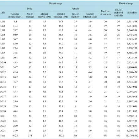
Table 1.
Summary of genetic and physical map of Pacific bluefin tuna.
Genetic map
Physical map
LGs
Male
Female
Total no.
of markers
No. of
anchored
scaffolds
Size (bp)
Genetic
distance (cM)
No. of
markers
Marker
interval (cM)
Genetic
distance (cM)
No. of
markers
Marker
interval (cM)
LG1
5.4
19
0.3
69.5
25
2.9
26
26
7,311,548
LG2
41.3
14
3.2
45.5
14
3.5
19
19
4,013,609
LG3
55.7
16
3.7
66.5
16
4.4
20
20
7,566,954
LG4
60.9
20
3.2
56.3
16
3.8
26
26
7,445,291
LG5
36.7
18
2.2
76.9
20
4.0
22
22
8,683,432
LG6
53.0
12
4.8
54.0
12
4.9
14
14
5,824,343
LG7
19.4
11
1.9
62.3
16
4.2
17
17
3,758,735
LG8
34.5
18
2.0
34.9
11
3.5
19
19
5,886,385
LG9
30.4
12
2.8
50.5
13
4.2
17
17
4,872,438
LG10
43.3
16
2.9
66.2
15
4.7
22
22
7,525,825
LG11
34.7
12
3.2
73.9
15
5.3
19
19
6,890,034
LG12
41.6
20
2.2
64.1
15
4.6
23
23
7,880,459
LG13
84.2
14
6.5
92.3
17
5.8
20
20
6,805,915
LG14
35.7
18
2.1
53.3
14
4.1
20
20
8,512,497
LG15
54.1
17
3.4
41.1
13
3.4
18
18
8,527,022
LG16
45.7
16
3.0
49.8
16
3.3
21
21
7,004,297
LG17
35.8
13
3.0
27.1
15
1.9
19
19
6,185,918
LG18
25.9
18
1.5
47.5
19
2.6
21
21
5,107,399
LG19
37.0
13
3.1
33.8
9
4.2
14
14
4,691,049
LG20
40.4
14
3.1
55.4
12
5.0
18
18
6,731,092
LG21
52.1
20
2.7
67.2
20
3.5
25
25
8,650,511
LG22
64.5
16
4.3
41.3
14
3.2
16
16
4,817,797
LG23
26.0
12
2.4
29.2
13
2.4
16
16
3,887,699
LG24
34.9
15
2.5
73.9
16
4.9
18
18
5,216,393
Figure 1.
Male and female genetic linkage maps of T. orientalis. Vertical squares represents Male (left) and Female linkage
group, respectively. Genetic distances between adjacent markers are shown above in Kosambi mapping function (cM).
Common marker between two sexes is bridged by connected lines. Markers with red asterisks (*) showed a significant
se-gregation distortion from the expected Mendelian 1:1 sese-gregation in female map.
00613_53311 00392_266915 00390_94555 00084_322090 1.1 00833_77351 00415_58321 1.1 00391_186975 49362_2269 00055_557397 00781_193138 00307_134557 00308_198364 00751_167377 00606_117549 00601_158674 2.2 00905_129588 00230_325570 1.1 00761_181066 00662_10641 LG1 5.4 cM 00875_106151 5.4 1.1 1.1 3.2 9.8 00052_385529 1.1 1.1 2.2 00771_194722 5.4 1.1 2.2 00319_291741 4.3 1.1 1.1 00729_16418 6.5 00847_127421 23.0 00916_67468 69.5 cM 00518_85385 1.1 00333_218804 2.2 01632_2485 00627_83670 00420_110640 2.2 00697_95618 3.2 00974_18978 4.3 01054_116762 4.3 00955_124695 7.6 00967_158089 2.2 01217_118109 14.4 01098_106052 01850_84397 01354_47986 LG2 41.3 cM 00934_70815 9.8 00411_197292 4.3 8.7 01263_44111 1.1 2.2 9.8 00101 439063 1.1 2.2 00615_146462 3.2 3.2 45.5 cM 00804_765 12.1 00809_161938 3.2 00944_65398 6.5 00185_18196 15.5 00038_356123 7.6 00044_557436 2.2 00479_164430 1.1 00094_323057 1.1 2.2 00255_110427 2.2 00033_575768 00010_781278 2.2 00203_136570 00982_115106 00408_171705 00492_109640 LG3 55.7 cM 14.4 1.1 2.2 00265_126950 5.4 8.7 2.2 1.1 00205_303932 7.6 00835_35085 12.1 2.2 8.7 00171_222856 1.1 00186_302547 66.5 cM 00926_178429 00525_73008 00450_64216 00457 145224 1.1 00302_117386 6.5 00449_190409 1.1 00747_77239 3.2 00735_142037 3.2 00344_229141 4.3 00360_144136 1.1 00894_115217 00095_365782 1.1 00090_474748 3.2 00899_61488 3.2 00298_179563 3.2 00279_163067 8.7 00397_124125 00661_199929 15.5 00857_38754 5.4 00758_136813 LG4 60.9 cM 2.2 6.5 00066_257637 1.1 1.1 00296_77766 2.2 00196_154314 1.1 00551_183042 2.2 1.1 7.6 1.1 10.9 7.6 3.2 00364_110919 3.2 00864_54093 5.4 56.3 cM 00075_95644 6.5 00115_267973 3.2 00023_682414 2.2 00174_235377 6.5 00050_328297 3.2 00193_210757 00839_21044 1.1 00714_19543 1.1 00500_1665 00153_401556 1.1 00034_183287 4.3 00380_65256 1.1 00361_142893 2.2 00646_39958 00126_455614 4.3 00049_329914 00053_380153 00770_193378 LG5 36.7 cM 4.3 00679_48521 6.5 1.1 00129_342326 1.1 00546_227598 1.1 1.1 7.6 2.2 10.9 7.6 8.7 10.9 1.1 2.2 4.3 4.3 00366_155573 2.2 146.1 cM 00103_228054 1.1 00123_167823 00169_177627 3.2 00645_157801 4.3 00162_313019 2.2 4.3 00109_128874 3.2 00069_102016 7.6 00018_365575 4.3 00452_238268 9.8 00125_425690 4.3 00909_89223 8.7 00760_109813 LG6 53.0 cM 2.2 3.2 7.6 3.2 6.5 00228_22684 5.4 6.5 7.6 4.3 00046_354953 5.4 2.2 54.0 cM 00259_38068 2.2 00609_215496 2.2 00119_335944 2.2 00154 270166 3.2 00414_248669 4.3 00048_150402 00128_315130 3.2 00118_445594 1.1 00498_193397 1.1 00189_278390 00783_22974 LG7 9.4 cM 00846_50838 10.9 4.3 5.4 5.4 3.2 3.2 00746_27380 6.5 00141_408598 1.1 2.2 17.9 00014_385141 2.2 00261_176016 00330_206854 62.3 cM 00477_3475 00430_55738 1.1 00293_239989 00915_183244 1.1 00513_127218 00280_100118 2.2 00213_68215 00685_2827 2.2 00532_28858 1.1 00650_71824 2.2 00856_1876 1.1 00463_73801 4.3 00232_301439 7.6 00009_514635 2.2 00078_132497 3.2 00184_263120 2.2 00988_100199 4.3 00795_9771 LG8 34.5 cM 34.9 cM
00182_47978 00589_151519 00791_125354 5.4 00542_22467 00559_232640 4.3 00577 13831 00677_116910 1.1 00745_120874 1.1 00379_34874 4.3 00249_88492 12.1 00550_31082 2.2 00239_273631 LG9 30.4 cM 00031_368460 1.1 00268_35309 6.5 1.1 00807_15806 12.1 00381_274354 3.2 17.9 1.1 7.6 00921_56424 55.9 cM 00994_81046 3.2 00087_101769 8.7 00285_91074 3.2 00352_17553 2.2 00145_238363 9.8 00208_257727 00372_156446 3.2 00578_32552 4.3 00006_761447 3.2 00370_6167100236_269275 2.2 00454_124238 00777_98600 1.1 00935_155990 2.2 00051_211304 00431_177546 LG10 43.3 cM 5.4 07445_1679 00549_102351 8.7 00165_248757 3.2 2.2 4.3 00284_267020 1.1 3.2 00058_544515 9.8 3.2 00384_241972 10. 9.8 4.4 66.2 cM 00097_394083 00502_177633 00231_259399 2.2 00301_147576 3.2 2.2 00287_212724 3.2 00526_103784 4.3 00263_250029 2.2 00438_221425 00933_85820 1.1 00030_319912 6.5 00815_144058 12.1 00740_129410 LG11 36.9 cM 00227_70020 5.4 00116_417144 4.3 00005_610364 9.8 00699_205382 8.7 2.2 00146_75017 3.2 3.2 14.4 9.8 1.1 2.2 00768_151767 7.6 00136_215754 2.2 73.9 cM 00289_110193 2.2 00930_14611 1.1 00220_35847 1.1 00878_146379 00552_45779 00663_53252 00336_277236 00488_15510 00317_245129 00142_277539 00167_150448 00739_156044 1.1 00524_24113 1.1 00351_225199 3.2 00056_277475 00076_171876 9.8 00248_41311 1.1 00210_54610 4.3 00060_449308 16.7 00841_157365 LG12 41.6 cM 13.2 00160_258703 5.4 3.2 4.3 10.9 4.3 1.1 00104_395600 6.5 5.4 00151_31055 1.1 8.7 64.1 cM 00962_9072 5.4 00858_125335 3.2 00221_265802 00042_205845 3.2 00035_115704 12.1 00353_80333 7.6 00385_3161 6.5 00244_137400 7.6 00388_5491 00820_135582 1.1 00403_159090 6.5 00703_106777 14.4 00762_180208 16.7 00654_73567 LG13 84.2 cM 1.1 6.5 7.6 2.2 00016_658769 7.6 5.4 1.1 3.2 00140_111707 7.6 00132_191501 10.9 2.2 00281_302083 2.2 00468_62179 12.1 12.1 5.4 5.4 00631_217115 92.3 cM 00017_135995 4.3 00491_193325 00020_291940 2.2 00134_312921 2.2 00828_109198 00931_32550 00340_211772 00303_288918 1.1 00981_113310 8.7 00419 162528 3.2 00093_24283 7.6 00147_105521 00099 435286 00004_886445 2.2 00122_266017 1.1 00105_119773 00032_435309 3.2 00471_29393 LG14 35.7 cM 15.5 8.7 1.1 3.2 5.4 2.2 00085_363474 3.2 00979_44555 3.2 3.2 1.1 6.5 53.3 cM 00355_85820 7.6 00910_65961 10.9 00080_298907 8.7 00039_394087 2.2 00329_44622 3.2 00111_291702 5.4 00063_195848 3.2 00026_267152 2.2 00036_456502 1.1 00363_133525 1.1 00022_661885 1.1 00008_803992 4.3 00911_167209 2.2 00197_295591 1.1 00045_218346 00072_331722 00441_269547 LG15 54.1 cM 00218_311412 8.7 3.2 3.2 3.2 2.2 1.1 4.3 2.2 1.1 10.9 1.1 41.1 cM 00597_49293 4.3 00436_19386 1.1 00970_154333 00895_124894 00027_603499 00059_177790 00083_506654 00096_85218 4.3 00194_309657 2.2 00790_149838 2.2 00257_230233 2.2 00121_314068 3.2 00245_310245 3.2 00541_245376 14.4 00684_16035 8.7 00418_158396 LG16 45.7 cM 00731_72616 3.2 5.4 7.6 9.8 5.4 00135_23239 2.2 1.1 00885_143593 2.2 1.1 1.1 00918_35163 1.1 1.1 00217_189367 8.7 49.8 cM 00859_104637 00332_70603 1.1 00181_145357 00708_100317 00732_205680 2.2 00159_126940 2.2 00845_96881 2.2 00251_176303 2.2 00120_340187 2.2 00711_149557 4.3 00127_236472 4.3 00963_169877 3.3 00062_36778 35.8 cM 00354_195889 1.1 00047_153600 6.6 00288_182806 1.1 3.2 00583_197206 4.3 00264_296767 2.2 5.4 3.3 00405_275398 27.1 cM 00183_234545 1.1 00325_150740 00591_222305 00814_163533 01267_129645 01894_59038 01223_104303 3.2 01045_146520 1.1 00374_206401 1.1 00098_401184 00529_11236 00496_15884 2.2 00386_215848 00665_91072 6.5 00741_134776 1.1 00778_204378 8.7 01564_12423 1.1 00616_69185 LG18 25.9 cM 1.1 4.3 01757_83020 1.1 5.4 3.2 3.2 3.2 00074_240980 2.2 6.5 1.1 2.2 2.2 3.2 1.1 00966_43581 7.6 47.5 cM 00647_18112 5.4 00246_232655 9.8 00082_412469* 3.2 00187_105168* 2.2 00673_147435* 00106_187871* 13.2 00091_276727 1.1 00817_131946 00342_217848 00283_163507 00522_93906 00311_2504*
2.2 00649_8071* LG19 37.0 cM 3.2 00161_292321 5.4 2.2 14.4 6.5 2.2 33.8 cM 01561_90042 14.4 00398_90943 9.8 00686_84565 3.2 00002_358935 7.6 00100_205743 00149_250489 3.2 00040_154055 1.1 00506_153914 1.1 00530_20686700269_183859 00641_95262 00349_117312 00816_37075 00267_5231 LG20 40.4 cM 13.2 00041_262465 8.7 3.2 8.7 1.1 2.2 2.2 5.4 00903_63693 3.2 00172_167230 1.1 6.5 00124_210364 55.4 cM 00940 5717 1.1 00322_215349 2.2 00324_45366 10.9 00114_369105 1.1 00634_187757 1.1 00021_81471 5.4 00175_169417 2.2 00079_517200 1.1 00387_110610 12.1 00013_638192 2.2 00065_349693 5.4 00112_219640 3.2 00539_199922 1.1 00763_149998 1.1 00252_284152 00973_74660 1.1 00362_103951 1.1 00657_186033 00466_201546 00902_75955 LG21 52.1 cM 3.2 1.1 4.3 00992_130518 4.3 5.4 00168_209325 6.5 00108_370173 14.4 5.4 1.1 4.3 2.2 2.2 1.1 1.1 00776_154787
The male map consisted of 24 linkage groups with 374 MS markers. The total length of the linkage groups
was 992.9 cM, and the mean distance between two markers was 2.7 cM. The sizes of individual linkage groups
ranged from 5.4 to 84.2 cM (mean, 41.4 cM). The number of markers per linkage group varied from 11 to 20,
with a mean of 15.6 markers per linkage group. The estimated genome coverage of the map was 86.5%.
The female map included 366 markers in 24 linkage groups. This map spanned 1332.3 cM, and mean spacing
between two markers was 3.7 cM. The sizes of the female linkage groups ranged from 27.1 to 92.3 cM (mean,
55.5 cM). The number of markers per linkage group varied from 9 to 25, with a mean of 15.3 markers per group.
The estimated genome coverage of the map was 86.5%.
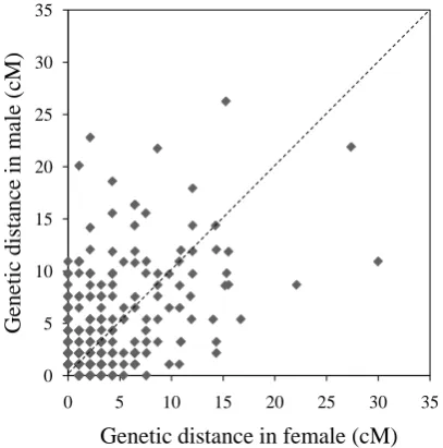
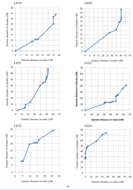
The ratio of male map length to female map length was 1.0:1.4. The distribution of the intervals between
con-tiguous common markers in both linkage maps was almost the same (
Figure 2
), although several linkage groups
clearly showed different recombination rates in specific regions or linkage groups (
Supplementary Figure S2
).
In particular, the genetic distance between the common markers in LG1, LG5, LG7, LG11, LG14, LG18, and
LG24 on the female map was higher than the male genetic distance. In contrast, LG15 and LG22 showed higher
genetic distances on the male map.
3.4. Mapping the Sex-Linked Sequence
The MS marker (07445_1679), which was developed in scaffold Ba00007445, was only polymorphic in females
and mapped to the LG10 terminal region on the female map (
Figure 1
). Orthologues of several sex-determining
genes in teleosts
[23]
but were not found on the LG10 scaffold of the integrated genetic linkage map.
3.5. Integration of the Genetic Linkage Maps with the Physical Map
Developing MS markers to specific regions of each scaffold allowed us to integrate the genetic and physical
maps into a consolidated genome map. We anchored 470 scaffolds to be consistent with the order of markers
determined on the genetic linkage maps. Thus, we placed scaffolds that cumulatively represented 20.8% (153.8
Mb) of the sequenced genome onto the linkage groups (
Table 1
). In total, 4243 genes estimated in the tuna draft
genome assembly have been included in these scaffolds
[8]
.
3.6. Comparison of Genome Structure in Other Teleosts
Constructing the integrated Pacific bluefin tuna map made it possible to compare conserved sequence regions
with those of other teleosts. We identified 6445 pairs of orthologous genes among tuna and four other teleosts
[image:7.595.212.416.486.692.2](fugu, medaka, stickleback, and
Tetraodon
). Then, we extracted 1381 gene pairs from these orthologous genes
Figure 2.
Recombination ratio between male map and female map. The common intervals
flanked by adjacent markers from the 24 linkage groups are compared.
0
5
10
15
20
25
30
35
0
5
10
15
20
25
30
35
G
en
et
ic
d
is
tan
ce
in
m
al
e (
cM
)
and mapped them on the integrated map. We constructed an Oxford grid
[35]
for Pacific bluefin tuna against the
four teleosts based on the number of orthologous genes on each linkage group/chromosome. These results
indi-cated that 24 pairs of chromosomes in tuna and medaka showed a clear one-to-one relationship (
Figure 3
).
Comparisons with the other three fish species also indicated highly conserved one-to-one relationships, although
there were several one-to-two and one-to-three relationships between homologous chromosomes. For example,
fugu chromosome 1 corresponded to LG3, LG19, and LG21 in Pacific bluefin tuna (
Figure 3(b)
). Stickleback
chromosome 1 corresponded to LG2 and LG13 in Pacific bluefin tuna. A similar result was observed in
stickle-back chromosome 4 with LG10 and LG23 in Pacific bluefin tuna (
Figure 3(c)
). Three one-to-two relationships
were detected between
Tetraodon
(chromosomes 1 - 3) and Pacific bluefin tuna (LG4 and LG10, LG19 and
LG21, and LG2 and LG8) (
Figure 3(d)
).
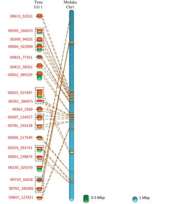
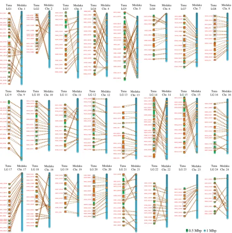
We constructed an integrated map to compare the Pacific bluefin tuna and medaka chromosome structures.
Homologous sequence regions across several chromosome pairs between tuna and medaka revealed reciprocal
homology relationships as well as reverse orientation orderings. Thus, several inversions may have occurred in
either genome (
Figure 4
and
Supplementary Figure S3
).
(a) (b)
(c) (d)
Figure 3.
Oxford grid comparing genomes of
T.
orientalis and four model fishes. Commonly conserved 1378 orthologous
genes among five fishes were plotted into Oxford grids. Each number in a cell indicates the number of orthologs in each
ge-nome. Each grids were drawn by specific color according to the number of orthologous, The number of each linkage group
of T. orientalis was determined in this study. (a) T. orientalis-Medaka comparison; (b) T. orientalis-Fugu comparison; (c) T.
orientalis-Stickleback comparison; (d) T. orientalis-Tetraodon comparison.
M ed ak a chr om os om es
1 2 3 4 5 6 7 8 9 10 111213 1415 161718 1920 212223 24
1 69 1 1 1
2 25
3 52 4
4 54
5 52
6 41
7 85
8 66
9 61 1
10 80
11 3 28
12 55 3
13 4 54
14 106
15 1 78
16 81
17 1 75
18 3
19 53
20 1 52
21 1 78
22 1 1 46 3
23 31 24 29
F
u
gu
chr
om
os
om
es
1 2 3 4 5 6 7 8 9 10 111213 1415 16171819 202122 2324
1769 1 1
8 25 1 3
13 34 20 53 19 52 9 41 3 85 5 65
21 61 1
14 80
12 3 29
6 55 3
11 4 54
15 106 1
4 1 78
7 81
22 76
10 52
1 19 1 1 1 53 77 4
2 1 46 3
18 31 16 29
S
ti
ck
leb
ack
ch
ro
m
o
so
m
es
1 2 3 4 5 6 7 8 9 10111213 1415161718 192021222324
9 70 1 1
2 53 4
8 54 17 52 19 41 12 85 11 66 13 61
4 80 31
10 3 29
14 56 3
1 4 25 54
7 106 3
6 79
20 81
3 76
5 53
21 52
16 1 78
15 1 46 3
18 29
T
et
raodon
chr
om
os
om
es
1 2 3 4 5 6 7 8 9 10 11121314151617181920212223 24
1868 1 1
5 53 4
11 52
13 41
9 85
3 25 1 66
12 61 1
1 52 78 1
21 3 1 28
4 55 3
16 4 51
7 106 1
17 1 78
8 81
15 75
20 2 1 3
6 52
2 1 1 53 77
10 4 46 3
19 31
14 1 29