Inflation as a function of labor force change rate: cointegration test for the USA

Munich Personal RePEc Archive

Inflation as a function of labor force

change rate: cointegration test for the

USA

Kitov, Ivan and Kitov, Oleg and Dolinskaya, Svetlana

IDG RAS

January 2007

Online at

https://mpra.ub.uni-muenchen.de/2734/

Inflation as a function of labor force change rate: cointegration test for the

USA

I.O. Kitov1, O.I. Kitov2, S.A. Dolinskaya1

Introduction

Inflation forecasting plays an important role in modern monetary policy in developed

countries. There is a trade-off between theoretical and practical aspects of the forecasting –.

Any practical application has to be based on a sound theoretical background, and every

theory must concentrate empirical facts and everyday practice in a few quantitative relations.

In reality, monetary authorities more often use expert judgments instead of theoretical

models. These judgements are often based on some concepts empirically proved to be wrong

such as the conventional Phillips curve, “expectation augmented” Phillips curve or NAURU

approach. As a matter of fact, there is no unique and comprehensive model in mainstream

economics and econometrics, which is able to explain observations and predict inflation in

developed countries.

A study of inflation as an economic variable driven solely by labor force change has

been carried out by Kitov (2006a-c, 2007) for the USA, Japan, France, and Austria. This

study has confirmed the existence of a linear relationship between inflation, unemployment

and labor force. In the USA, the inflation-labor force relationship is characterized by a

two-year time lag. Regression analysis (Kitov, 2006b) has shown a high level of correlation

(R2>0.9) between the variables and the lowermost, among available forecasting models, out-of-sample root-mean square forecasting error (RMSFE) at a two-year horizon, which

corresponds to the observed lag. An important advantage of the model consists in its perfect

parsimony - single predictor is used to fit observations in several countries during the last 25

to 45 years. Moreover, autoregressive properties, extensively used in many economic and

econometric models of inflation, are not necessary because the relation between labor force

change and inflation is strict. It does not allow any deviation between observed and predicted

inflation when both variables are measured precisely.

As a consequence, the existence of a strict link between inflation and labor force

1

Institute for the Dynamics of the Geospheres, Russian Academy of Sciences

2

change denies the concept of rational expectation thoroughly adopted in economics, i.e.

future values of inflation are known to the extent some past values of labor force level are

known. At the same time, the strict relation allows for a partial inflation control through labor

force control and provides clear foundations for a sound economic policy.

Both variables are non-stationary, however, implying a possibility for the regression

results to be spurious ones despite the existence of a theoretical background (Kitov, 2006b,

2007) based on the fact that personal income distribution in the USA does not change with

time when normalized to the total population and GDP. Therefore, econometric tests are

necessary whether the relationship between inflation and labor force is a cointegrating one.

The cointegration between inflation and labor force change would mean that the results of the

previous regression analysis hold from the econometric point of view. For the USA,

cointegration analysis is essentially a bivariate one. This significantly simplifies the

implementation of relevant analysis and statistical inferences. However, in the case of

modeling inflation using labor force change rate, a straightforward application of

econometric methods potentially leads to wrong conclusions.

The rest of the paper is organized in four sections and one appendix. Section 1 briefly

introduces the model and presents some results obtained for the USA in the previous study.

Section 2 is devoted to the estimation of the order of integration in measured inflation and

labor force change rate. Unit root tests are carried out for original series and their first

differences. GDP deflator represents inflation in the study.

In Section 3, the existence of a cointegrating relation between the measured and

predicted inflation is tested. The latter is represented by four time series reflecting

improvements in the accuracy of prediction associated with suppression of random noise in

the labor force readings. The presence of a unit root in the difference (residual) between the

measured and predicted inflation implies the absence of cointegration between the variables

and a strong bias in the results of the previous regression analysis. The residuals obtained

from regressions of the measured inflation on the predicted ones are also tested for the unit

root presence. This approach is in line with that proposed by Engle and Granger (1987).

The maximum likelihood estimation procedure developed by Johansen (1988) is used

to test for the number of cointegrating relations in a vector-autoregressive representation

smoothness – from the original predictor to its three-year moving average. VAR and

vector-error-correction models (VECM) are estimated for the forecasting purposes.

Section 4 discusses the principal results and their potential importance for economic

theory and practical application, and concludes. Appendix introduces a pre-determined

variable (from linear to a quasi-stochastic one) trend, which is of a crucial importance for

cointegration study of time series related to population estimates such as labor force level.

1. The static model

There is a unique link between inflation and labor force change rate in the USA as obtained

for the last 45 years (Kitov, 2006c). In econometric sense, it is a long-run equilibrium

relation or static model which uses only original values of the involved parameters not their

first differences. It is advisable to use the rate of labor force growth (not increment) as a

predictor in order to match the dimension of inflation – [t-1]. An implicit assumption of the model is that inflation does not depend directly on parameters associated with real economic

activity. Moreover, inflation does not depend on its own previous and/or future values

because it is completely controlled by a force of different nature – by the dynamics of the

portion of population participating in labor force.

As defined by Kitov (2006a), inflation is a linear and potentially lagged function of

labor force change rate:

(t)=A1dLF(t-t1)/LF(t-t1)+A2 (1)

where (t) is the inflation at time t, LF(t) is the labor force level at time t, t1 is the time lag

between the inflation and labor force, A1and A2 are country-specific coefficients, which have

to be determined empirically. The coefficients may vary through time for a given country as

different units of measurements (or definitions) of the studied variables are used, but for true

values of inflation and labor force they are constant.

Linear relationship (1) defines inflation separately from unemployment. This

representation is an adequate one for the purpose of the paper. However, inflation and

unemployment are two indivisible features of a unique process (Kitov, 2007). The process is

channels. The first channel is the increase in employment and corresponding change in

personal income distribution (PID). All persons obtaining new paid jobs or their equivalents

presumably change their incomes to some higher levels. There is an ultimate empirical fact,

however, that the US PID practically does not change with time in relative terms, i.e. when

normalized to the total population and total income (Kitov, 2005a,b). The increasing number

of people at higher income levels leads to a certain disturbance in the PID. This

over-concentration (or over-pressure in physical terms) of population in some income intervals

above its neutral value must be compensated by such an extension in corresponding income

scale, which returns the PID to its original density. Related stretching of the income scale is

called inflation (Kitov, 2006a). The mechanism responsible for the income scale stretching,

obviously, has some relaxation time, which effectively separates in time the source of

inflation, i.e. the labor force change, and the reaction, i.e. the inflation itself.

The second channel is inherently related to those persons in the labor force who tried

but failed to obtain new paid jobs. These people do not leave the labor force joining

unemployment. Supposedly, they do not change the PID because they do not change their

incomes. Therefore, the net labor force change equals the unemployment change plus the

employment change, the latter process expressed in economies as the lagged inflation.

Kitov (2006c) proposed to estimate coefficients in (1) not by a linear regression of

inflation on labor force change rate. Such a regression balances measurement errors, i.e. the

deviations from a true relationship, through the entire period of observations (between 1960

and 2004) and has two important drawbacks: estimates of linear regression coefficients are

usually biased due to errors in the predictor and the influence of larger fluctuations is

overestimated. The latter might be of a higher importance in our case, considering the

practice of revisions carried out by the US Bureau of Labor Statistics (BLS) and the Census

Bureau (CB).

An alternative to regression arises from the fact that the labor force level is actually

measured in monthly surveys not the change rate. Absolute uncertainty associated with

annual measurements of the labor force level is constant or improving with time. Therefore,

relative uncertainty associated with the net change in the labor force level during a given

period is inversely proportional to the net change. When the net change in labor force level is

improvement in the accuracy of the estimates of cumulative values. Considering

measurement errors, a simple summation of annual estimates is always less accurate than a

direct measurement of corresponding levels. (In the case of labor force, however, the

revisions conducted by the BLS effectively cancel corresponding measurement errors out

through time and provide practically the same accuracy of cumulative change for both the

summation and the net level change techniques.) Therefore, the best-fit coefficients in (1)

have to provide the same cumulative values for the measured and predicted inflation at the

end of period, the latter having a decreasing uncertainty with time. This procedure should

result in somewhat more accurate estimates, which are also different from those obtained by

a standard linear regression. The estimated long-run relationship between inflation and labor

force for the USA is as follows (Kitov, 2006c):

π(t)=4.0*dLF(t-2)/LF(t-2)-0.03075 (2)

The left-hand side of the equation is called below the measured inflation, πm(t) , and the

right-hand side – the predicted one, πp(t). A statistical assessment of the linear relationship

carried out for the USA indicates that RMSFE of inflation forecasts at a two-year horizon for

the period between 1965 and 2002 is only 0.8%. This value is superior to that obtained with

any other inflation model, including the random walk approach, by almost a factor of 2. The

entire period was also split into two segments before and after 1983. The forecasting

superiority is retained with RMSFE of 1.0% for the first (1965-1983) and 0.5% for the

second (1984-2002) sub-period.

There is one aspect not analyzed in the previous papers - both variables are

non-stationary. Hence, validity of the regression results is under doubt (Granger & Newbold,

1967). When regressed, two I(1) processes may show unreasonably high correlation or

goodness-of-fit and severely biased estimates of corresponding regression coefficients. This

might happen to the studied relationship despite the sound theoretical foundation linking such

macroeconomic variables as real GDP growth and inflation to population parameters only

(Kitov, 2005ab, 2006ad). These links are treated as “mechanical” ones; i.e. any change in

defining population parameters is always fully transmitted into a strictly proportional change

There are several predicted inflation time series obtained by Kitov (2006c) for GDP

deflator and CPI measurements using corrected labor force readings. Corresponding

corrections in labor force level include redistribution of step-like revisions to population

controls carried out by the US CB and the BLS. These corrections smooth original labor

force series (SA) and effectively removes the largest spikes from its first difference.

Probably, the only exception is the years between 1990 and 1993, when an unprecedented

number of revisions to population estimates and labor force survey methodology were carried

out. The standard procedure of redistribution failed to iron the spikes out. So, the corrected

labor force time series still contains an artificial spike near 1990. (The revision carried out by

the BLS in July 2006 effectively resolved the problem of 1993, however.)

The set of the predicted time series also includes the one based on half-year shifted

labor force measurements. This time series is better synchronized with inflation

measurements because it averages monthly readings from July to June of the next year with

December being in the middle of the period. The shifted series gives a larger R2 than the original one presented by the BLS (Kitov, 2006c).

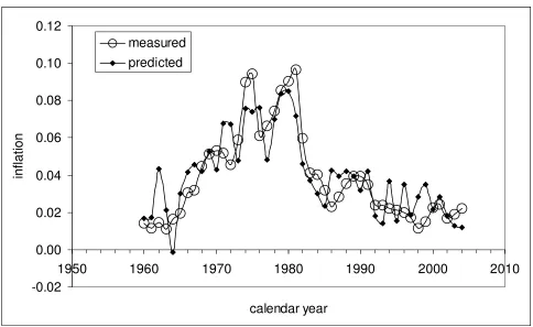
2. The unit root tests

It is clear from the behavior of the measured and predicted (in fact, labor force change rate)

inflation curves displayed in Figure 1 that both time series are potentially characterized by

the presence of unit roots because they demonstrate some clear non-stationary features.

Moreover, the cumulative measured and predicted inflation curves are definitely

non-stationary with a strong (stochastic or deterministic) trend component. In such a situation, a

spurious regression is probable as modern econometric research shows. Therefore, some

specific tests have to be carried out in order to prove validity of the results obtained in Kitov

(2006b,c). In particular, one has to prove that the measured and predicted time series are

integrated of order one, I(1), and are cointegrated, i.e. the residuals of their regression or

VAR representation create a stationary, I(0), series which meets a number of specific

requirements (Hendry&Juselius, 2001).

From statistical point of view, the principal problem of the econometric analysis

related to the relationship between inflation and labor force change consists in the balance

statistical tests work relatively well with time series of several hundred readings. When the

size of a sample is small, statistical inferences based on asymptotic distributions provided

with econometric packages may be biased. The replacement of asymptotic distributions by

those obtained specifically for small samples reduces the power of the tests. Increasing the

number of readings via sampling rate one observes decreasing accuracy. When measurement

uncertainty is high no useful signal (i.e. long-term relationship) can be retrieved from the

noise. There is no general solution of the problem and one always has to compare the

outcome of statistical tests with the bulk of external information - theoretical and empirical.

As a first step in the analysis, we have to prove that the measured and predicted

inflation are I(1) processes. There is a number of standard unit root tests provided with many

econometric packages – the Dickey-Fuller, the Augmented DF (ADF), the modified DF t-test

using a generalized least-squares regression (DF-GLS), Phillips-Perron and others. From this

set, we use only the ADF and DF-GLS because the DF has a skewed distribution with a long

left tail complicating discrimination the null of a unit root, and the PP test works better

asymptotically, i.e. is not reliable at short time series. Standard programs of Stata9 statistical

package are used in the current study.

There are several time series modeled in (Kitov, 2006c), which may be potentially

tested for the unit root presence: the measured inflation (GDP deflator and CPI inflation) for

the period between 1960 and 2004 (45 readings); numerous time series predicted from the

labor force change rate (dLF/LF) – original, shifted by half a year, and those smoothed by

moving average of various width. All the predicted time series are also present in two

intervals: from 1958 to 2002 and from 1960 to 2004. The latter series are the versions of the

former ones but shifted by two years ahead in order to synchronize the predicted inflation

readings with corresponding measured values because of the two-year lag. The original

predicted series retain the actual lead ahead of the measured values important for causality

tests. Because the original and the two-year shifted time series differ by four values (each of

the series contain two readings different from its counterpart) one may potentially expect a

slightly different result of the unit root tests. From all available time series, measured and

predicted, only those associated with the annual readings of GDP deflator are studied here.

Table 1 lists results of the ADF and DF-GLS tests for a unit root in the measured

predicted time series which are shifted by two years ahead. The series measured represents

the GDP deflator time series between 1960 and 2004, the series predicted and shifted are

synchronized (shifted by two years ahead) with the measured one, and the original (not

shifted) predicted series are titled as predicted2 and shifted2. The last raw in the Table lists

1% critical values for corresponding tests. For the DF-GLS test, only values for lags 1 and 4

are presented because results for lags 2 and 3 are very close to those for lag 4.

One can derive an overall conclusion from Table 1 that no one series is a stationary

one because the null of the unit root presence can not be rejected. It is worth noting that the

predicted series shifted by two years, such as the predicted and predicted2, actually give

different but close results. It does not affect the general conclusion of non-stationarity,

however.

The series displayed in Table 1 are non-stationary. But it does not mean that these

series are I(1) and some additional efforts are necessary to prove the assumption. For an I(1)

process, the first difference has to be a I(0) process. Therefore, the same tests are repeated on

the first differences of the two principal time series – dmeasured and dpredicted, which are

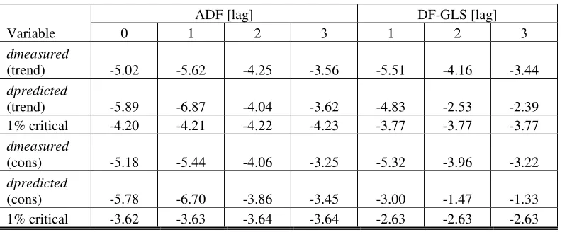
displayed in Figure 2. Corresponding test results are presented in Table 2.

A standard unit root test usually contains many specifications related to various

features potentially present in time series. The tests listed in Table 2 use two different

assumptions on the presence of constant and trend in the first differences. First, we allow for

a deterministic linear trend in the processes and test for a single unit root in an AR(p)

representation, where p=0,1,2,3 for the ADF test and p=1,2,3 for the DF-GLS test. All the

tests for the dmeasured, except those with lag 3, imply the rejection of the null of the unit

root presence at the 1% level. For the dpredicted, only tests with lags 0 and 1 reject the null.

The presence of a constant term is a more reasonable hypothesis for the first

differences of such processes as inflation and labor force change. When a constant

specification is used in the ADF unit root tests, results are more favorable for the rejection of

the null for both dmeasured and dpredicted. For the DF-GLS, the null is rejected for all lags

in the dmeasured and only for lag 1 in the dpredicted. Because of the mixed results for the

dpredicted, more information is necessary for rejection or acceptance of the null.

Here we have to draw a bold separation line between the procedures for estimation of

information on prices. There are some short-term corrections related to the inflation

measurements which incorporate late information and new methodology. There is no

correction extended far in the past, however, which is dependent on new inflation readings.

Thus, one can consider subsequent readings of inflation as relatively independent in view of

the measuring procedures.

This is not the case with the labor force measurements, however. The labor force

level is estimated in monthly surveys using some limited population samples. Simultaneous

estimates of age-gender-race distribution, then converted into population controls, are used

for mapping the limited sample results onto the entire population. Such a construction of the

labor force estimates has two drawbacks – the sample changes are slow in order to study the

dynamics of the inter-sample evolution, and the population controls are determined both

from the monthly-quarterly-yearly population estimates and decennial censuses.

The sample stability implies the presence of a link between subsequent labor force

estimates. Corrections to the population controls are of even larger influence on labor force

readings, however. After every decennial census, the BLS conducts severe (sometimes

several per cent) revisions of the population age structure, which are extended long in the

past. These revisions effectively include synchronized changes in the population controls

over the entire period. Figure 3 demonstrates a remarkable effect of such revisions on the

change in the number of people in a one-year-wide population cohort – the difference

between 15-year-olds and 14-year-olds a year before. This age is of importance for the labor

force measurements because statistics starts at 15 years of age. Therefore their influx is one

of the defining components of the labor force increase along with net migration and total

deaths. The difference between the numbers is everything but of a natural shape. Considering

the disturbances introduced into the labor force time series by the BLS one should not be

surprised that the DF-GLS tests does not reject the null for the first difference of the

predicted inflation, which is based on the labor force change rate. Some statistical properties

of population time series important for the cointegration analysis are discussed in Appendix.

The dmeasured time series is characterized by a very low average (0.00019±0.011)

compared to the "min" and "max" values of -0.036 and +0.031. Slope and intercept of the

regression on time are -0.00012±0.00012 and 0.24±0.24, respectively, i.e. the null of zero

and intercept and the assumption of constant specification is applicable to the previous tests.

The overall conclusion is that the dmeasured serieshas no unit root and the dpredicted series

would not have a unit root if not the artificial distortion induced by the labor force

measurement procedure. Therefore, the original series measured and predicted are integrated

of order one.

3. The cointegration tests

The assumption that inflation and labor force change in the USA are two cointegrated

non-stationary time series is equivalent to the assumption that the difference between the

measured and predicted inflation, ε(t)=πm(t)−πp(t), is a stationary or I(0) process. It is natural

to start with a unit root test in the difference. If ε(t) is a non-stationary variable having a unit

root, the null of the existence of a cointegrating relation can be rejected. Such a test is

associated with the Engle-Granger's approach, which requires πm(t)to be regressed on πp(t)

as the first step, however. Since the predicted variable is obtained by a procedure similar to a

linear regression and provides the best fit for cumulative values, we skip the regression and

start with an analysis of the difference.

The hypothesis of a unit root is tested by the same procedures as before – the ADF

and DF-GLS. If the null of a unit root is rejected, the hypothesis of no-cointegration is also

rejected. In this case, the equilibrium relationship between the measured and predicted

inflation is valid and a vector error-corrected model can be estimated using the results of the

first stage.

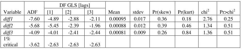
Table 3 presents some results of the unit root tests. There are three differences tested:

diff1=(πm(t)- πp(t)), diff2=(πm(t)-MA(2)), and diff3=(πm(t)-MA(3)). The ADF and DF-GLS

results indicate the absence of a unit root in the diff1 residual series, except may be for lag 3

in the DF-GLS tests. The diff1 series of the largest importance because it is based on the

inflation predicted from the original labor force series. As discussed in Section 2 and

Appendix, the labor force measurements are potentially biased by a strong autocorrelation

introduced by the revisions to the population controls. One can expect the enhancement of

the autocorrelation in the differences (Chiarella&Gao, 2002). Moreover, this autocorrelation

has to be more prominent in the smoothed series, where random noise in measurements is

series diff2 and diff3 illustrate these effects – the DF-GLS tests produce the results which are

higher than corresponding 1% critical values also listed in the Table. So, smoothing leads to

deterioration in the test results compared to those for the original series.

It is worth noting that the moving average time series provide a better description of

the observed inflation as represented by standard deviation in the residual series. The best fit

is obtained for the MA(3) series with standard deviation twice as low as that provided by the

original predicted series: from 0.017 for diff1 to 0.009 in diff3. The price paid for the better

description is higher values in the unit root tests. Therefore, one can obtain a wrong statistical

inference by over-suppressing of the stochastic component in real data, as shown in

Appendix. Concluding the discussion, we reject the null of the unit root presence in the three

difference series.

The next step is to use the Engle-Granger's approach and to study statistical properties

of the residuals obtained from linear regressions of the measured inflation on various

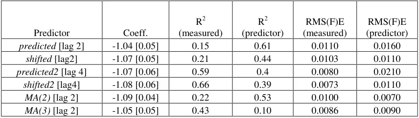
versions of the predicted inflation. Table 4 summarizes principal results of the regression

analysis – coefficients with their standard deviations, R2, RMS(F)E (F stays for forecasting because of the two year lag), and t for the null of zero coefficients. The dependent variable is

always the measured series and predictor varies from the predicted to MA(3). Results of

specification tests on heteroskedasticity, omitted variables, ARCH effects, and serial

correlation, also listed in Table 4, indicate that the residuals of the regressions, except those

related to MA(3), meet the requirements defining I(0) process and have properties of a

white-noise realization necessary for a VAR representation of the measured and predicted inflation.

Therefore, one cannot reject the null that the dependent variable and the predictors are

cointegrated. The reasons for the failure of the specification test for MA(3) have been already

discussed.

The Johansen's (1988) approach is based on the maximum likelihood estimation

procedure and tests for the number of cointegrating relations in the vector-autoregressive

representation. The above analysis has shown that the VAR representation is an adequate one

due to the properties of the regression residuals. The Johansen's approach allows

simultaneous testing the existence of cointegrating relations and determining their number

(rank). For two variables, only single cointegrating relation is possible. When cointegration

both variables have to be stationary. Thus, when the Johansen test results in rank 1, a

cointegrating relation does exist.

Table 5 lists trace statistics, eigenvalues, LL and other information obtained from the

cointegration rank tests for a number of predictors and trend specifications. The maximum

number of lags included in the underlying VAR model is 4 in all tests. No null of

cointegration rank 1 can be rejected. So, there is a cointegrating relation between the

measured and predicted inflation.

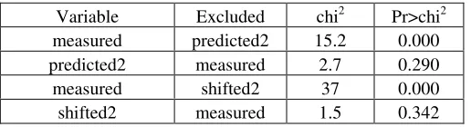
Because of the two-year lag behind the labor force change and the existence of the

cointegrating relation or long-run equilibrium relationship (2), a test on causality direction is

a trivial one. In this test, the variables predicted and shifted are replaced with their original

version predicted2 and shifted2, which leads the measured variable by two years. Results of

the causality tests are presented in Table 6, which demonstrates that the predictors are weakly

exogenous variables.

Now we are sure that the measured and predicted inflation series are cointegrated and

the principal results of the previous research hold. Therefore, the estimates of the

goodness-of-fit and RMSFE are accurate. The estimates were obtained in a simplified regression

procedure, which does not use autoregressive properties of noise. A standard moving average

smoothing provides a substantial suppression of the noise, as the increase in R2 from 0.7 for the annual readings to 0.9 for MA(3) demonstrates (Kitov, 2006c).

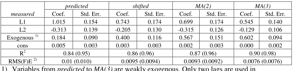
A VAR representation may potentially provide a further improvement due to

additional noise suppression. In practice, AR is a version of a weighted moving average,

which optimizes noise suppression throughout the whole series. In the VAR model, we use

the shifted2 series as an exogenous predictor and the maximum lag 4 instead of the

pre-estimated one maximum lag 3. The level of correlation between the measured and predicted

series does not allow any past values of inflation to influence the present ones and, hence, the

past values of labor force change. The equilibrium relationship is a strict one and converges

to a unique curve when measurement errors are eliminated. At any time, inflation does not

contain information important for labor force change. So, the labor force change rate is an

exogenous variable. One cannot deny the influence of current inflation on current labor force

The distribution of the VAR error term is close to the normal distribution with

skewness=-0.05 and kurtosis=3.99, the former being of much higher importance for the

Jarque-Bera normality test and validity of statistical inference. The VAR stability is

guaranteed by the eigenvalues of the companion matrix lower than 0.54. There is practically

no autocorrelation at lags from 1 to 4 as follows from the LM statistics. Therefore the VAR

model accurately describes the data and satisfies principal assumptions on the residuals.

A VECM representation uses additional information to that provided by the VAR

models due to separation of noise and equilibrium relationship. So, it potentially provides an

improvement on the VAR models. Tables 7 and 8 list some results of the VAR and VECM

for a number of predictors. There is only a marginal improvement in RMSFE on that

obtained by the linear regressions. The smallest RMSFE is 0.0076 in the VAR representation

(MA(3) as a predictor) and 0.0073 in the VECM representation (shifted2 as a predictor). The

best RMSFE from the linear regressions for the period between 1965 and 2002 is 0.008.

One can conclude that these powerful statistical methods fail to improve on the

simple predictions. A significant decrease in the forecasting uncertainty is possible only

through a major increase in the accuracy of inflation and labor force measurements. This

conclusion is in line with a standard research cycle in hard sciences.

4. Conclusion

The core result of the analysis consists in formal statistical confirmation of the existence of a

unique linear and lagged (two years for the USA) relationship between inflation and labor

force change. Hence, the two I(1) variables are cointegrated in statistical sense; i.e. their

residual time series is proved to be a stationary one with white noise characteristics - no unit

root, normal underlying distribution, no omitted variables, no autocorrelation, no

heteroskedasticity. The absence of such cointegration test was a weak point in the previous

papers. It exposed the results of modeling and theoretical consideration to criticism.

Observed inflation is always a combination of two components – a pre-determined

variable trend (demonstrating stochastic features), which one-to-one repeats the behavior of

some true labor force change, and a noise component related to measurement errors in both

In terms of physics, there is a process "mechanically" linking true inflation to true

labor force change. Observed deviations from the relationship describing the mechanical link

are measurement errors. The long-run equilibrium relationship implies the absence of any

structural breaks necessary for the explanation of the changes in the US inflation observed

during the last 50 years. Such structural breaks are a common feature of a majority of models

developed in the econometric framework, where inflation is considered as a stochastic

process.

The noise component demonstrates some artificial features related to the procedures

used by the US BLS for the labor force estimation. As in hard sciences, improvements in the

measurement procedures, both for inflation and labor force, can potentially provide any

desired accuracy of inflation forecast at a two-year horizon and even further if to improve the

accuracy of labor force projections. It is worth noting that there is no error-correction

mechanism associated with the deviations of true inflation values from the true predicted

ones, but there exist error-correction mechanisms, which compensate random and systematic

errors through time. For the labor force series, this mechanism is obviously associated with

multiple revisions, which reshape the error pattern, in amplitude and timing, at very long

time horizons.

The long-run relationship between inflation and labor force change rate is explained

by the reaction of personal income distribution on the disturbance induced by those persons

who enter employment and change their incomes correspondingly. This consideration is a

part of the new economic concept, which relates macroeconomic variables to quantitative

Appendix. Variable deterministic trend

In hard sciences, situations where a non-stationary time series practically repeats the

behavior of another series with some time lag are common. Finding of such a resemblance is

a first step of a variety of research programs. The next natural step is to reduce the level of

noise associated with measurement errors. For a scientist, this step is necessary for obtaining

a higher confidence in the existence of a strict link between two variables or in the absence of

such a link. So, improving measurement accuracy results in the acceptance of a true

relationship or in the rejections of a false one.

In econometrics, however, the presence of such a pre-determined variable trend often

leads to deterioration of the performance of standard statistical procedures associated with

non-stationary processes. The danger to wrongly reject the presence of a true link in standard

econometric procedures is associated with a general rejection of the existence of real

deterministic trends in economic time series except the simple ones as connected to

economic growth. Such simple trends are easily removed by detrending procedures.

Otherwise, there exist only stochastic trends in econometrics, which represent the central

problem in analysis of non-stationary time series. In some cases, this assumption leads to a

biased result. For example, when correlation between two series in strong and random

measurement errors are significantly suppressed, even small systematic errors induced by

estimation procedures become defining for rejection of cointegration, i.e. for rejection of the

true link between the variables.

There are several key assumptions, which lay in the basement of the cointegration

concept. One of them is associated with the properties of residuals necessary for two or more

non-stationary processes to be cointegrated. The existence of a cointegrating relation means

that the residual of some linear combination of non-stationary variables is stationary. This

residual time series has to be an independent and identically distributed with zero mean and

constant variance, IID(0, 2), where IID is not necessary the normal distribution. Such residuals guarantee unbiased estimates of relevant coefficients.

The mainstream research of cointegration phenomenon allows for some deterministic

trend in non-stationary variables which is very often considered as a linear or quadratic one.

The inclusion of such trend terms sometimes helps to distinguish between purely stochastic

studies of more complicated cases with nonlinear deterministic trends. But most of them

consider analytic functions. Here we extend the notion of deterministic trend to the level of

deterministic variable (potentially stochastic) process, i.e. to such a process, which has

stochastic statistical properties but is fully pre-determined. In physics, this notion is similar to

decomposition of a measured time series into true and noise components.

The importance of deterministic variable trend for econometrics can be illustrated by

a simple but principal example associated with the discussion in Section 2 of growth in the

number of 15-year–olds in the USA, N15(t). The evolution of this number is definitely

described by a stochastic time series, supposedly, by I(2) process. In the framework of

econometrics, this implies that the expected value of the change in N15 is zero (if to exclude

a small deterministic trend):

N15(t)-N15(t-1)=dN15(t)=ε(t) (A1)

where ε(t) some stochastic ID(0,σ2) process. (Actual dN15 average value between 1960 and 2004 is 29900 and standard deviation is 193000. If to exclude the years between 1960 and

1962, the mean=14500 and stdev=115000.) Thus, dN15(t) must have very low level of

autocorrelation for the small time series under consideration. Asymptotically, autocorrelation

at any lag must be zero – E[(ε(t)*ε(t-s)]=0 for any s 0. In fact, autocorrelation associated

with the actual series of dN15(t) between 1960 and 2004 is below 0.25 at lags from 1 to 15.

Therefore, the annual increment in the N15(t) can hardly be predicted from its previous

values. This is a standard situation in econometrics, which deals mainly with economic and

financial variables. A general convention dictates that there is no way to exactly predict the

forthcoming change in stock prices or CPI inflation. Only statistical estimates are available.

This is not the case with the dN15(t), however.

First, one has to learn some statistical properties of the N15. Figure A1 shows the

annual N15 readings, the first difference, dN15, and also the second differential d2N15.

(There are also N0 and N14 and their differentials shown in the Figure.) Due to strong

variations in the number of 15-year-olds in the earlier 1960s we limit the N15 series to the

The ADF test rejects the null of a unit root in the d2N15 time series and accepts the

null for N15 (for lag 0 and larger) and dN15 (for lag 1 and larger). The DF-GLS tests for the

same series assume the acceptance of the null in the d2N15, however (see Table A1). Thus,

the problem of a unit root in the d2N15 is a controversial one and needs more attention to the

population estimation process. For our purposes, we reject non-stationary in the d2N15.

Regardless of the unit root presence in the N15 and its stochastic properties, one can

accurately predict its value at a one (and more) year horizon using the change in the number

of 14-year-olds one year ago, dN14(t-1)=N14(t-1)-N14(t-2), as a proxy to the

dN15(t)=dN14(t-1)+ω(t), where ω(t) is associated with the differences in death and

migration rate between 14-year-olds and 15-year-olds in the given year. Another way to

obtain an accurate estimate of the N15(t) is to update N14(t-1) by the inflation-deflation

method used by the Census Bureau in the population estimates. Actually, the N15(t) contains

the same population cohort, by the year of birth, as the N14(t-1) plus net migration, m(t), and

less total deaths, ρ(t), in the population of the given age. Therefore, one can rewrite

relationship (A1) in the following forms:

N15(t)=N15(t-1)+dN14(t-1)+ω(t) (A2)

N15(t)=N14(t-1)+ρ(t)+m(t) (A3)

Relative importance of ω(t) can be estimated from the difference between dN15(t) and

dN14(t-1) normalized to the dN14(t-1), as presented in Figure A2. The shape of the curve is

not a surprise because of multiple revisions made by the USA Census Bureau. The years

between decennial censuses are characterized by low values (<0.1) of the ratio

(dN15(t)-dN14(t-1))/dN14(t-1) indicating that the fraction of the dN15(t) not explained by the

dN14(t-1) is very small. Therefore, the net effect of ω(t) is below 10% for those 7 to 8 years when

the disturbance induced by population revisions after decennial censuses is low.

The years around the censuses demonstrate a highly volatile behavior of the ratio.

Such a behavior has a clear explanation – new counts obtained in decennial censuses have to

be accommodated into new population estimates. As a rule, old (so-called postcensal)

population estimates show age structures different from those obtained in the censuses for the

year of age populations. Unfortunately for our approach, the breaks are made simultaneously

in all age groups. As a result, the number of 14-year-olds one year ago is not corrected in the

same way as the number of 15-year olds in the given year and their difference demonstrates a

spike. One can eliminate such spikes by introducing an appropriate correction into the

N14(t-1), which can be effectively the same as the correction in the N15(t).

When the spikes near the census years are removed, the difference N15(t)-N14(t-1)

(and hence, the difference dN15(t)-dN14(t-1)) still looks biased as Figure A3 demonstrates.

There are three intervals with constant differences: from 1981 to 1990, from 1991 to 2000,

and after 2000, and one interval with a positive linear trend - between 1963 and 1980. Such a

behavior apparently results from the methodology used by the Census Bureau to balance the

total population growth over the whole age structure. It is difficult to believe, however, that

the difference evolves in such a deterministic way. On the other hand, this deterministic

behavior can be eliminated from the difference by subtracting the mean values in the periods

of constant difference and by compensating the trend between 1963 and 1980. Figure A3

displays the corrected difference which now fluctuates around the zero line and has no trend.

The mean value of the corrected difference N15(t)-N14(t-1) for the period between 1963 and

2004 is zero and standard deviation is only 2200 or 1.5% of that of that in dN15.

Thus, we found that a number of reasonable corrections can provide an almost precise

estimate of the difference between the N14(t-1) and N15(t). The two terms in (A3) associated

with deaths and migration are decomposed in a deterministic and stochastic component, the

former being effectively attached to the deterministic trend term N14(t-1). Theoretically, one

can consider this combination as a pre-determined variable trend - it demonstrates stochastic

properties but is completely known in the given year t. In practice, one can use the current

trend in the difference N15(t)-N14(t-1) (Figure A3) and current estimates of the N14(t) for a

prediction of the N15(t+1),t=2007,…,2010.

The same statement is valid for the first differences of the N15(t) and N14(t-1), where

the latter is the pre-determined variable trend of the former. A very conservative amplitude

estimate of the residual stochastic component of the difference u(t)=dN15(t)-dN14(t-1)

would be 0.05dN14(t-1), i.e. u(t)=o(dN14(t)) for our purposes (see Figure A4). Such a small

high level of correlation between the variables. A linear regression gives R2=0.98, the slope of 0.996±0.003 and intercept 18±471.

The number of 15-year-olds is of a special importance in economics. This number

represents a principal component of the annual increase in labor force along with effects of

participation rate, net migration and deaths. Therefore, one can expect the labor force level

demonstrating the existence of a nonzero deterministic variable trend. In addition to the

pre-determined, according to (A2) or (A3), influence of the N15(t), the labor force participation

rate is characterized by a high degree of predictability, at least during the last 45 years.

Figure A5 shows a period of practically linear growth between the 1960s and the

mid-1990s induced by the active growth in the women’s participation rate. In fact, a linear trend

shown in the Figure explains more than 97% of the variability in participation rate during the

period. The last five years are characterized by a slight downward trend in the participation

rate. The USA BLS, the CBO and a number of other agencies and institutions provide a wide

range of projections at various time horizons associated with the participation rate and labor

force itself.

It is time to recall that the dN15(t) and dN14(t-1) series are I(1). For many economic

and financial non-stationary time series, a regression of two I(1) processes may be spurious,

i.e. to give severely biased estimates of regression coefficients and R2. In our case, there is no doubt that the variables are practically identical and the estimates of the linear regression

coefficients and goodness-of-fit are consistent. This implies that the variables have to be

cointegrated, i.e. the difference between them has to be a I(0) process.

The estimation of cointegration rank in the framework of the Johansen's VAR

methodology shows, however, that there is no cointegrating relation between the variables.

Table 2A lists results of the cointegrating rank tests for the original and corrected series

dN15(t) and dN14(t-1). The tests reject the existence of any cointegration, i.e. cointegration

rank 1, in both cases. This outcome, while surprising, obviously belongs to the type I

spurious regression (Chiarella&Gao, 2002), i.e. rejection of a true relation. Such wrong

rejection is driven by the artificial statistical properties of the difference between the

variables induced by the Census Bureau revisions – original and those left after the

cointegrated, but the corrected series are integrated. It implies that two I(2) processes, as

follows from the unit root tests of their first differences, have a I(0) difference.

Such situations deserve a special consideration in the framework of econometrics.

Before starting any statistical study one has to be absolutely sure that the residual or errors

are of significant amplitude. In some cases, residuals characterized by high autocorrelation

and other possible statistically “wrong” properties should not prevent acceptance of strong

correlation between economic variables. This is especially important for the variables

associated with population surveys, where means are used in order to enhance these "wrong"

statistical properties. Labor force estimates are not an exclusion from the list.

As a synthetic example of such a behavior, several time series are constructed

mimicing principal features of the population and labor force estimates. A reference time

series is described by the following function: r(t)=0.3sin(0.1t), where t=1,…,45. Sinus

function provides a degree of non-stationarity, when tested for the unit root presence, and has

a period roughly corresponding to that of actual population time series: ~30 years. A

piece-wise systematic error term of various amplitude but the same time structure is added to the

reference function. Time dependence of the error term is described by constants of 10-year

length with changing sign: e(A,t)=A*(-1)int(0.1*t+1), where A is coefficient varied from 0.005 to

0.1 in the study, int(.) is the integer part of the value in the brackets. The 10-year intervals

correspond to decennial censuses.

So, we test for cointegration between the following time series: r(t) and r(t)+e(A,t) as

a functions of A. First, the reference series is regressed on the disturbed series. As expected,

goodness-of-fit is excellent: R2 from 0.999 for A=0.005 to 0.784 for A=0.1. There is no doubt that the regression is not a spurious one in physical terms – the curves practically coincide.

There is an obvious problem with statistical tests. One can expect that the residuals of the

regression demonstrate strong, and independent on A, autocorrelation prohibiting the

existence of a cointegrating relation between the studied functions, before A is large enough

to avoid co-linearity threshold predefined in every statistical package. In fact, the

Durbin-Watson test gives an almost constant value around 0.36 and LM tests for autoregressive

conditional heteroskedasticity consistently rejects the null of no ARCH effects.Obviously,

statistical tests give excellent results regardless the goodness-of-fit because the regression

residuals now have properties of white noise.

This consideration is a trivial one from the point of view of econometrics and would

not deserve any further efforts to be wasted. In reality, one often is not aware of specific

properties of actual time series and still has to rely on statistical tests. Actual measurement

noise very probably contains an artificial component, such as the periods of a constant

difference observed in the population estimates, and a random component. Supposedly,

relative amplitude of the latter is decreasing due to improving procedures. The random

component can be also suppressed by smoothing. Therefore, the artificial component

becomes defining for statistical estimates at some point. This definitely happens, when

moving average is applied to smooth the labor force estimates. Goodness-of-fit increases,

RMSE decreases, the predicted curve converges to the measured one, and … statistical tests

References

Chiarella, C., & Gao, S. (2002). Type I spurious regression in econometrics. Working Paper No 114, School of Finance and Economics, University of Technology Sydney Granger, C., & Newbold, P. (1967). Spurious regression in econometrics. Journal of

Econometrics, 2, 111-120

Engle, R., & Granger, C. (1987). Cointegration and error correction: representation, estimation, and testing. Journal of Econometrics, 55, 251-276

Hendry, D., & Juselius, K. (2001). Explaining Cointegration Analysis: Part II. Energy Journal, 22, 75-120

Johansen, S. (1988). Statistical analysis of cointegrating vectors. Journal of Economic Dynamics and Control, 12, 231-254

Kitov, I. (2005a). A model for microeconomic and macroeconomic development. Working Paper 05, ECINEQ, Society for the Study of Economic Inequality

Kitov, I. (2005b). Modeling the overall personal income distribution in the USA from 1994 to 2002. Working Paper 07, ECINEQ, Society for the Study of Economic Inequality Kitov, I. (2006a). Inflation, Unemployment, Labor Force Change in the USA. Working Paper

28, ECINEQ, Society for the Study of Economic Inequality.

Kitov, I. (2006b). The Japanese economy. Available at SSRN: http://ssrn.com/abstract=886663 Kitov, I. (2006c). Exact prediction of inflation in the USA. Available at SSRN:

http://ssrn.com/abstract=916060

Kitov, I. (2006d). GDP growth rate and population. Working Paper 42, ECINEQ, Society for the Study of Economic Inequality.

Tables

Table 1. Unit root tests of the measured (GDP deflator) and predicted inflation in the USA

DF GLS [lags] Variable

ADF

[lag 0] [1] [4]

measured -1.57 -1.93 -1.46

predicted -3.53 -1.95 -1.22

shifted -1.95 -2.10 -1.48

predicted2 -3.46 -2.14 -1.55

shifted2 -1.73 -2.19 -1.52

MA(2) -1.50 -2.18 -1.32

MA(3) -1.40 -1.65 -1.45

Table 2. Unit root test of the first differences of the measured and predicted inflation

ADF [lag] DF-GLS [lag]

Variable 0 1 2 3 1 2 3

dmeasured

(trend) -5.02 -5.62 -4.25 -3.56 -5.51 -4.16 -3.44 dpredicted

(trend) -5.89 -6.87 -4.04 -3.62 -4.83 -2.53 -2.39 1% critical -4.20 -4.21 -4.22 -4.23 -3.77 -3.77 -3.77 dmeasured

(cons) -5.18 -5.44 -4.06 -3.25 -5.32 -3.96 -3.22 dpredicted

Table 3. Unit root test of the differences between the measured and predicted inflation

DF GLS [lags]

Variable ADF [1] [2] [3] Mean stdev Pr(skew) Pr(kurt) chi2 Pr>chi2

diff1 -7.60 -4.89 -2.88 -2.11 0.00095 0.017 0.36 0.18 2.76 0.25

diff2 -5.68 -5.45 -2.39 -1.96 0.00088 0.012 0.39 0.46 1.34 0.51

diff3 -4.09 -4.01 -2.41 -2.44 0.00081 0.009 0.26 0.84 1.36 0.51

1%

Table 4. Results of tests for heteroskedasticity, omitted variables, ARCH effects, and serial correlation as applied to the residuals of linear regressions of variable measured on four predictors.

Predictor

Hettest 1) Pr>chi2

Ramsey 2) test Pr>F

LM for ARCH 3)

Pr>chi2

Breusch-Godfrey LM 4) Pr>chi2

DW 5)

d-stat R2 RMS(F)E

Cons [cons] Pr>|t|

Predicted 0.21 0.0046 0.80 0.13 1.61 0.62 0.015

0.012 [0.004]

0.004

Shifted 0.25 0.0029 0.97 0.18 1.58

0.79

(0.94) 0.012

0.005 [0.003]

0.15

MA(2) 0.13 0.043 0.37 0.12 1.55

0.83

(0.95) 0.010

0.0014 [0.003] 0.66

MA(3) 0.29 0.0065 0.88 0.008 1.16

0.86

(0.96) 0.0095

0.0008 [0.003] 0.78 1) H0 - constant variance; 2) H0 - no omitted variables; 3) H0 - no ARCH effect; 4) H0 - no

Table 5. Cointegrating rank of a VECM

predictor

trend

specification rank parms LL eigenvalue

trace statistics

5% critical

value

predicted constant 0 14 242.5 . 25.77 15.41

predicted constant 1 17 254.0 0.427 2.9037* 3.76

shifted constant 0 14 265.3 . 21.08 15.41

shifted constant 1 17 274.6 0.365 2.4773* 3.76

predicted rconstant 0 12 242.5 . 25.81 19.96

predicted rconstant 1 16 253.9 0.428 2.9282* 9.42

shifted rconstant 0 12 265.2 . 21.19 19.96

shifted rconstant 1 16 274.6 0.366 2.4830* 9.42

predicted none 0 12 242.5 . 22.68 12.53

predicted none 1 15 253.6 0.419 0.4437* 3.84

shifted none 0 12 265.2 . 18.29 12.53

Table 6. Granger causality test

Variable Excluded chi2 Pr>chi2 measured predicted2 15.2 0.000 predicted2 measured 2.7 0.290

measured shifted2 37 0.000

Table 7. VAR results for the measured GDP deflator.

predicted shifted MA(2) MA(3)

measured Coef. Std. Err. Coef. Std. Err. Coef. Std. Err. Coef. Std. Err.

L1 1.015 0.154 0.743 0.174 0.699 0.174 0.545 0.140

L2 -0.313 0.139 -0.205 0.130 -0.315 0.126 -0.129 0.106

Exogenous 1) 0.184 0.090 0.400 0.116 0.567 0.151 0.602 0.094

cons 0.005 0.003 0.003 0.003 0.002 0.003 0.000 0.002

R2 0.84 (0.95) 0.86 (0.96) 0.87 (0.96) 0.90 (0.98)

RMS(F)E 2) 0.01 (0.010) 0.0095 (0.0094) 0.0093 (0.0092) 0.0076 (0.0076) 1) Variables from predicted to MA(3) are weakly exogenous. Only two lags are used in

every case.

Table 8. VECM results for the measured GDP deflator

Predictor Coeff.

R2 (measured)

R2 (predictor)

RMS(F)E (measured)

RMS(F)E (predictor)

predicted [lag 2] -1.04 [0.05] 0.15 0.61 0.0110 0.0160

shifted [lag2] -1.07 [0.05] 0.21 0.44 0.0103 0.0110

predicted2 [lag 4] -1.07 [0.06] 0.59 0.4 0.0080 0.0210

shifted2 [lag4] -1.08 [0.06] 0.66 0.39 0.0073 0.0110

MA(2) [lag 2] -1.09 [0.04] 0.22 0.53 0.0100 0.0070

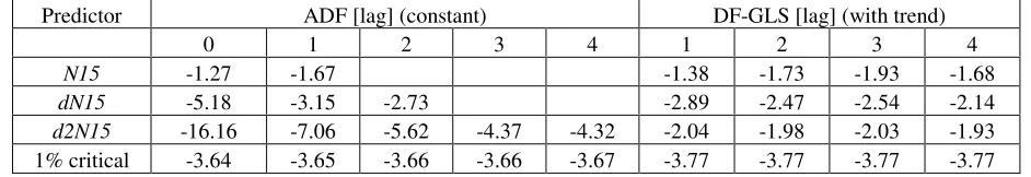
Table A1. Results of the ADF and DF-GLS tests for N15, dN15, and d2N15

Predictor ADF [lag] (constant) DF-GLS [lag] (with trend)

0 1 2 3 4 1 2 3 4

N15 -1.27 -1.67 -1.38 -1.73 -1.93 -1.68

dN15 -5.18 -3.15 -2.73 -2.89 -2.47 -2.54 -2.14

d2N15 -16.16 -7.06 -5.62 -4.37 -4.32 -2.04 -1.98 -2.03 -1.93

Table 2A. Results of cointegration rank test.

Specification [cons] [trend] [none]

rank 0 1 0 1 0 1

dN15(t) vs. dN14(t-1) original 36.62 11.61 39.05 11.61 35.95 11.22

dN15(t) vs. dN14(t-1) corrected 48.29 9.49 48.39 9.47 47.96 9.16

N15(t) vs. N14(t-1) original 11.60* 2.62 12.58* 1.65 7.61* 0.16

N15(t) vs. N14(t-1) corrected 26.72 2.75* 26.83 2.85* 23.71 0.21*

Figures

Figure 1. The measured and predicted time series between 1960 and 2004. The labor force estimates are obtained at the BLS web-site in July 2006. Therefore the strong spike near 1993 discussed in (Kitov, 2006c) has disappeared.

-0.02 0.00 0.02 0.04 0.06 0.08 0.10 0.12

1950 1960 1970 1980 1990 2000 2010

calendar year

in

fl

a

ti

o

n

Figure 2. The series dmeasured and dpredicted obtained as the first differences of the

measured and predicted in Figure 1.

-0.05 -0.04 -0.03 -0.02 -0.01 0.00 0.01 0.02 0.03 0.04

1950 1960 1970 1980 1990 2000 2010

calendar year

in

fl

a

ti

o

n

Figure 3. The difference between N15(t) and N14(t-1) in the USA for the period between 1960 and 2004

-1.0E+05 -5.0E+04 0.0E+00 5.0E+04 1.0E+05 1.5E+05

1960 1970 1980 1990 2000 2010

calendar year

#

a)

0.0E+00 1.0E+06 2.0E+06 3.0E+06 4.0E+06 5.0E+06

1880 1900 1920 1940 1960 1980 2000 2020

calendar year

#

0 14 15

b)

-1.0E+06 0.0E+00 1.0E+06 2.0E+06

1950 1960 1970 1980 1990 2000 2010

calendar year

#

c)

-5.0E+05 0.0E+00 5.0E+05

1965 1975 1985 1995 2005

calendar year

#

d2N0 d2N15

Figure A1.

a) The number of 15-, 14-, and 0-year-olds as a function of time between 1900 and 2004. Notice a large step in the earlier 1960s in the 15- and 14-year-olds corresponding to the burst in birth rate after the WWII.

b) The first differences of the time series presented in panel a). The step near 1960 is transformed into a spike, which is associated with natural causes. The spikes near the years of decennial censuses are of artificial character.

-1.0E+00 -5.0E-01 0.0E+00 5.0E-01 1.0E+00

1960 1970 1980 1990 2000 2010

calendar year

#

(dN15-dN14)/dN14

y = 0.3899x - 773.17

-60000 -40000 -20000 0 20000 40000 60000 80000

1950 1960 1970 1980 1990 2000 2010

calendar year

#

corrected

original

Figure A3. The original (open circles) and corrected (solid diamonds) difference between

1.0E+00 1.0E+01 1.0E+02 1.0E+03 1.0E+04 1.0E+05 1.0E+06

1950 1960 1970 1980 1990 2000 2010 2020

calendar year

#

dN14(t-1)

dN15(t)-dN14(t-1) av(dn14)

av(dN14-dN15)

y = 0.2814x - 493.95 R2 = 0.9743

55 60 65 70

1950 1960 1970 1980 1990 2000 2010

calendar year

p

a

rt

ici

p

a

ti

o

n

r

a

te

,

%