Munich Personal RePEc Archive
Forecasting in vector autoregressions
with many predictors
Korobilis, Dimitris
University of Strathclyde
January 2008
Online at
https://mpra.ub.uni-muenchen.de/21122/
Forecasting in vector autoregressions with many
predictors
Dimitris Korobilis
University of Strathclyde
Working Paper, January 2008
Abstract
This paper addresses the issue of improving the forecasting performance of vec-tor auvec-toregressions (VARs) when the set of available predicvec-tors is inconveniently large to handle with methods and diagnostics used in traditional small-scale mod-els. First, available information from a large dataset is summarized into a consid-erably smaller set of variables through factors estimated using standard principal components. However, even in the case of reducing the dimension of the data the true number of factors may still be large. For that reason I introduce in my analy-sis simple and efficient Bayesian model selection methods. Model estimation and selection of predictors is carried out automatically through a stochastic search vari-able selection (SSVS) algorithm which requires minimal input by the user. I apply these methods to forecast 8 main U.S. macroeconomic variables using 124 potential predictors. I find improved out of sample fit in high dimensional specifications that would otherwise suffer from the proliferation of parameters.
Keywords: Bayesian VAR, forecasting, model selection & averaging, large datasets
JEL Classification: C11, C32, C52, C53
1. INTRODUCTION
It is common practice today to collect observations on many variables that potentially help explain economic variables of interest such as inflation and unemployment. Tech-nological progress has allowed the collection, storage, and exchange of huge amounts of information without much effort and cost. In turn, this has significantly affected recent macroeconomic modeling techniques. Current academic research is focused on finding solutions on how to efficiently handle large amounts of information with, for example, Stock and Watson (2002) using 215 predictors to forecast 8 major macroeconomic vari-ables for the U.S. economy. Bernanke and Boivin (2003), among others, argue that this is also the case nowadays in central banks, where it is customary for researchers and de-cision makers to monitor hundreds of subsidiary variables during the dede-cision-making process.
These reasons justify the current trend in applied modeling with large datasets. The modern econometrician has tools adequate enough to successfully extract information from hundreds of predictor variables and compute more accurate forecasts than ever before. It is noteworthy that these tools mainly do not rely on economic theory in an explicit way; rather they are statistical and consequently atheoretical methods that are used to cover the unfortunate gap between theoretical models and their empirical validation. Within the sum of all possible options, two methods in particular have re-cently gained ground: dimension reduction and model averaging. Among many others, Bernanke et al (2005), Favero et al (2005), Giannone et al (2004), Stock and Watson (2002, 2005a, 2005b) and Koop and Potter (2004) show how forecasts can be im-proved over univariate or multivariate autoregressions, using either dynamic factors or Bayesian model averaging (BMA), or both techniques, when a rich dataset is in hand.
In this paper I examine empirically the merit of using factors extracted from a large set of explanatory variables and at the same time implementing Bayesian model aver-aging/selection in the context of macroeconomic vector autoregressions (VARs). While factor methods have already been examined thoroughly in multivariate models, the challenging task of model averaging/selection is implemented with a stochastic search variable selection algorithm (henceforth SSVS) proposed by George and McCulloch (1993, 1997) and George et al (2008).
liter-ature on different approaches to BMA in VARs (Strachan & van Dijk, 2007; Andersson & Karlsson, 2008). The innovation of the specific prior formulation is that it is more appropriate for VAR models compared to previous model selection priors used in mul-tivariate regressions (Brown et al., 1998, 2002). That is because each right-hand side variable is allowed to enter in all, some, or none of the VAR equations, and not only in all or none of them. The additional advantages come from the fact that this class of restriction search algorithms is extremely simple to use and automated. Furthermore, certain versions of these algorithms can incorporate variable selection when the number of predictors is larger than the number of time series observations.
The following section defines the Bayesian VAR model when many variables are available. Within this “large model approach” the large number of variables is replaced with a small number of factors and several aspects of this approach are discussed. In Section 3, the stochastic restriction search is introduced as a means of efficiently se-lecting a subset of macroeconomic variables or factors that should be restricted from the VAR specification, based only on the information in the data. The prior specifica-tion necessary for model selecspecifica-tion is analyzed, as well as the interpretaspecifica-tion of model selection probabilities as a special case of BMA. Section 4 outlines the setting of the empirical section (data, forecasting models, prior hyperparameters, and comparison statistics), and the results of the forecasting performance of various VAR specifications. Section 5 concludes the paper with a summary and thoughts for further extension of the basic framework presented in this paper.
2. METHODOLOGY
Letytbe an m 1vector of variables of interest (that we want to forecast) observed for
t= 1; :::; T. Unlike previous univariate studies (Stock & Watson, 2002, Koop and Potter,
2004),m >1and I define a forecasting model foryusing a general VAR representation
y0
t+1 =
p1
X
i=0
y0
t iai+w
0
tc0+" 0
t+1 (1)
where the parameter matricesaiandc0are of dimensionsm mandN mrespectively,
yt i, i = 1; :::; p1,are lagged values of the dependent variable, wt is a N 1 vector
errors are iid Gaussian, "t N(0; ).This model can be estimated both by OLS and
Bayesian methods, provided that the total number of explanatory variables will not
exceed the total number of time series observations T. I propose to adopt a Bayesian
setting which allows for a unified treatment of this model in high dimensions. For a review of the VAR under standard prior specifications and different sampling methods, the reader is referred to Kadiyala and Karlsson (1997).
Assume we have available observations xt = (x1t; :::; xnt)
0
on some macroeconomic
quantities, where n is large (in the order of hundreds). A popular and simple method
to incorporate into an econometric model all the information inherent in a large set of
variables, is to reduce their dimension into a lower-dimensional vector of k n latent
factors and insert these in the VAR model as explanatory variables
x0
t = f
0
t +u
0
t (2)
y0
t+1 =
p1
X
i=0
y0
t iai+ p2
X
j=0
f0
t jbj+"t+1 (3)
where ft is an k 1 vector of unobserved factors, is the matrix of factor loadings
andutareiidnormal errors,ut N(0; W). In equation (3) the same assumptions hold
as in the base model in (1), with the only difference that now wt = (ft 1; :::; ft p2)
0
and N = k (p2+ 1), and the bj are of appropriate dimensions. For simplicity xt is
demeaned which is equivalent to imposing a constant term in the factor equation, equal
to the sample meanx= T1 Pxt(which in this model coincides both with the MLE of the
constant or the mode of its posterior under a diffuse prior). The factors are unobserved quantities and usually it is assumed that they follow a normal distribution with diagonal covariance matrix. One more convention in the factor model literature is to impose the
covariance matrix of the innovations, W, to be also diagonal so that (2) reduces to
independent equations. Estimation methods vary from principal component analysis (PCA) to full likelihood-based approaches. The ultimate goal of using the factor model
is to obtain the factor scoresft as a valid reduced representation of the manifest vector
xt, so that factor identifiability issues play no actual role here and will not be further
discussed.
In terms of the general forecasting VAR model in equation (1), I replace the
predic-torswtwith the principal components (PC) estimates of the factorsFbt=
h b
ft;fbt 1; :::;fbt p2
i
the dynamic factor model (or factor-augmented VAR) used in Bernanke et al (2005). From their point of view, the dynamic factor model (DFM) is treated as a state-space model, which has the advantage of a probably more efficient one-step estimation of the factors (i.e., along with the parameters of the model) through the Kalman filter algo-rithm. But this comes at a huge computational cost which makes the application of this model prohibitive in the recursive forecasting setting adopted in this study. After all, Stock and Watson (2005a) have already implemented a large-scale forecasting exercise involving DFMs where they compare several frequentist, full Bayes, and empirical Bayes approaches.
The factors replace the original variables in order to allow richer dynamics and
subsequently are allowed to have up to p2 + 1 lags. If the original observed series
xt = (x1t; :::; xnt)
0
were included as predictors then – for a typical macroeconomic dataset with monthly observations on many variables – a degrees of freedom problem would occur if more than one or two lags were assumed. However, even in the case of reducing the dimension of our data with factors the fact that we would ideally allow for
many lags does not resolve the problem of overparameterization. ForN =k (p2+ 1)
larger than 20 the number of all possible models will tend virtually to infinity so that pairwise comparison is practically infeasible using an AIC/BIC-type criterion or prior predictive (marginal) densities and Bayes factors. A reasonable proposed solution from a Bayesian point of view is to use shrinkage subjective priors. For example, the Min-nesota prior imposes restrictions on parameters which correspond to higher order lags
of y, whereas the prior weight (i.e., the prior mean) for the parameter on the first own
lag in each of the m equations is equal to one, and zero on the first lag of the rest
m 1dependent variables. While this approach will work well in VARs which include
only lags of the dependent variables, it is difficult to adopt this approach in the models examined here. This happens because there is no theoretical or empirical justification for constructing a subjective prior on exogenous predictor variables, especially if these exogenous variables are latent (constructed) factors.
should be based mainly on economic theory. The problem with this approach is that in many cases economic theory has empirically proven to be bad guidance in proposing relevant predictors. Stock and Watson (2003) argue that this is the case when forecast-ing inflation: “the literature does suggest [ . . . ] variables with the clearest theoretical justification for use as predictors often have scant empirical predictive content.”
The discussion so far has focused on the “large-n” case, avoiding to mention
any-thing about how small or large the dimensionmof the dependent variableyshould be.
Although macroeconomic VARs typically contain as dependent variables three or four fundamental quantities that describe the economy, when forecasting, the actual number of variables of interest can grow large. A decision maker would be interested to forecast future values of many series, like production, employment/unemployment, short- and long-term interest rates, consumer and producer price inflation, exchange rates, and many other nominal or real quantities. This is easily handled with the model selection algorithm which is the focus of the next section. The methods described below apply
to large VARs in a general sense, that is (i) when the number of predictors n grows
large and the number of dependent variables m is small, (ii) when m grows large and
n is small, or (iii) when bothm; n! 1, although the empirical application is centered
upon the first case.
3. BAYESIAN MODEL SELECTION AND AVERAGING
As was mentioned in the introductory section, when the number of candidate models is too large to enumerate, posterior sampling methods are necessary for the computation of marginal likelihoods for model comparison. Stochastic search algorithms that base on a Markov chain on model space identify regions of high posterior probability and can be used for model selection or to obtain posterior weighted estimates for model av-eraging. When applied to small models, these algorithms have the ability to search the entire model space, while in large settings only more plausible models are visited. An indicator (zero/one) variable , epitomizes the core of Bayesian model selection using
stochastic search techniques. Let us define the vector = ( 1; :::; s) as the complete
set of indicators, where s is the maximum number of parameters in the model. Then
we can proceed by defining a priorp( )which combined with the likelihoodp(dataj ),
will give zero or one value for each i, i = 1; :::; s, from the (updated based on data)
in-formation for model selection and averaging. The main idea is to impose the vector of
parameters, say = ( 1; :::; s), to have a structure conditional on the values of , so that
when i = 1the associated parameter i will be estimated according to its unrestricted
posterior density, and when i = 0this would imply i = 0.
There are many ways to implement this general strategy and many alternative meth-ods exist which involve several prior specifications. An analytical review of model av-eraging and selection is offered in Hoeting et. al (1998) and Chipman et al. (2001). A computationally fast restriction search is described in this section which is based on the SSVS algorithm of George and McCulloch (1993, 1997).
Define zt = yt0; y
0
t 1; :::; y 0
t p1; w
0
t
0
, then the VAR model in familiar matrix form is
obtained by stacking the row vectorsyt+1,ztand "tfort = 1; :::; T
y=z +", " N(0; ) (4)
where y= y0
2; :::; y 0
T+1 0
,z = [z0
1; :::; z 0
T]
0
, = [a0; :::; ap1; c0], and"= "
0 2; :::; "
0
T+1 0
. Note
that when forecasts are projectedh-steps ahead,yis the matrixy= y0
1+h; :::; y
0
T+h
0
(see
next section for a definition). Let nu = m (m (p1+ 1) +k (p2+ 1)) be the total
number of elements in ' = vec( ). From these elements the m in total constants are
always included in the models and admit a typical normal prior of the form
('c) N 'c; vIm (5)
where 'c is the block of ' which contains the constant terms. Let 'k be the vector of
the remainingn' =nu mparameters in' which are subject to restriction search and
let = 1; :::; n be the vector of indicator variables associated with the elements
of 'k. Then each element 'k
i conditional on i, i = 1; :::; n', follows a scale mixture of
normals prior of the form
'kij i (1 i)N 0; 20i + iN 0; 21i (6)
The hyperparameters 0i, 1i are selected in such a way so that 20i is small (or even
zero) and 2
1i is large. Subsequently each parameter 'ki is restricted with zero prior
mean and very small (or zero) prior variance when i = 0, while for i = 1has a large
(locally uninformative) prior variance and in that respect is left unrestricted.
updated by the information in the data. Hence a Bernoulli prior on these variables is placed, which updated by the likelihood will result in a conditional posterior which is
also Bernoulli. The elements of the vector follow an independent Bernoullipi 2(0;1)
prior of the form
( ) Yp i
i (1 pi)(1 i), i= 1; :::; n' (7)
This prior choice reduces computational costs and leads to a posterior density which is
easy to derive. In this case p( i = 1) = pi = 1 p( i = 0) so that pi reflects the prior
belief that 'k
i is large enough and should be left unrestricted. By selecting pi < 1=2,
models with an unreasonably large number of parameters are downweighted in order
to highlight the significance of parsimonious models. The special case wherepi = 1=28
i, is equivalent to a constant uniform priorp( ) 1=2n'. This prior is uninformative in
the sense that it favors each parameter equally; see Section 4.2 in this paper for more details, and the discussion in Chipman et al. (2001).
The hierarchical mixture prior described above is straightforward to interpret and can be applied virtually to any model for which a normal prior can be specified3 as the conjugate prior that leads to easy derivation of the underlying posterior. A differ-ent version of the SSVS is used in Brown et al. (1998) for a multivariate regression model used to predict three variables using 160 predictors. Following the suggestions of George and McCulloch (1997) and Smith and Kohn (1996) they set in equation (6)
2
0i = 0 and 21i = g z
0
z 1. This prior implies that the first component of the
mix-ture is a Dirac delta function at zero, i.e., a function that puts point mass at zero and
hence whenever i = 0, 'k
i will be exactly zero. The second component is Zellner’s
g-prior specification and suggestions for setting uninformative values ofg (although in
a univariate context) are given in Fernandez, Ley, and Steel (2001). An updated and computationally more efficient version of this prior specification appears in Brown et al. (2002), where more variables than observations can be handled. The shortcoming of their approach is that it is able to treat each equation in the VAR individually, but
instead is choosing the variables inz which are more probable to be included inallVAR
equations together. Put simply, if, say,z contains only the first lag of the dependent
vari-ables, then the latter approach will allow theyit 1 to be a predictor of the whole vector
yt, while the approach proposed hereyit 1to explain the dependent variable in equation
j of the VAR (denoted yjt), but not the dependent variable in the l-th VAR equation
(denotedylt). Nevertheless, the Brown et al. (2002) implementation of the SSVS
empirical analysis with focus on prediction.
Smith and Kohn (2002) extend the stochastic search for parameter restrictions to the covariance matrix of longitudinal data. George et al. (2008) apply their idea to the covariance matrix of structural VARs: motivated by the fact that identifying restrictions on the covariance are usually imposed on the elements of a reparametrization of , they
focus on restricting the elements of them m upper triangular matrix satisfying
1 = 0
(8)
They then derive a mixture of normals prior, as in equation (6), for the nondiagonal
elements of , while the diagonal is integrated out with a gamma prior. Matrix has
the form = 2 6 6 6 6 6 4
11 12 1m
0 22 . .. ... ..
. . .. ... 0
0 0 mm
3 7 7 7 7 7 5 (9)
so let = ( 11; :::; mm)
0
and = ( 0
2; :::; 0
m)
0
= 12; 13; 23; :::; (m 1)m
0
be the
vec-tors of the diagonal and upper diagonal elements respectively, where j = 1j; :::; (j 1)j
0
for j = 2; :::; m. Let!j = !1j; :::; !(j 1)j
0
be a vector of 0-1 variables so that each
ele-ment of j has prior conditional on !j of the form
ijj!ij (1 !ij)N 0; 02ij +!ijN 0; 21ij (10)
for i = 1; :::; j 1 and j = 2; :::; m. As in the case of the vector , assume that the
elements of the vector ! = (!0
2; :::; ! 0
m)
0
are independent Bernoulliqij 2 (0;1)random
variables so that
(!) Y
i
Y
jq !ij
ij (1 qij)(1 !ij) (11)
Fori= 2; :::; m, each iihas a gamma prior density
2
ii Gamma( i; i)
restrictions imposed in structural VARs. It should be clear from the prior specification that the SSVS is an intuitive extension of the Bayesian conjugate (normal – inverse Wishart) prior. In the empirical application I adopt a fast sampling scheme (see Section 4.2) to draw from the posteriors of c and x, which makes computation feasible in mul-tivariate models. The parameter posteriors are given in detail in Appendix A (Technical Appendix). Although selection of prior hyperparameters seems to be fairly automatic in this setting, prior elicitation is an important factor in model selection.
4. EMPIRICAL APPLICATION
4.1 Data
I use the Stock and Watson (2005b) dataset which is an updated version of the Stock and Watson (2002) dataset that is widely used in empirical applications. This version consists of 132 monthly variables pertaining to the US economy measured from 1960:01 to 2003:12. The 132 predictors can be grouped in 14 categories: real output and in-come; employment and hours; real retail, manufacturing, and trade sales; consumption; housing starts and sales; real inventories; orders; stock prices; exchange rates; interest rates and spreads; money and credit quantity aggregates; price indexes; average hourly earnings; and miscellaneous. The data were transformed to eliminate trends and non-stationarities. All the data and transformations are summarized in Appendix B.
4.2 Selection of prior hyperparameters
Implementation of Bayesian model selection requires all the priors to be proper, as the ones described in Section 3. Noninformative improper priors are not suitable to calculate Bayes factors and posterior model probabilities. Even though there are certain methods which overcome this difficulty (BIC approximations, intrinsic, or fractional Bayes factors), the standard practice in the Bayesian model selection literature is to use only proper priors. This does not necessarily mean that noninformative proper priors cannot be specified. It is easy to choose the hyperparameters in such a way that all the priors are locally noninformative.
Selection of 0i, 1i and 0ij, 1ij can be made along the guidelines of Chipman et al.
weighting can be allocated to those values of for which 'k
i > i when i = 1, iff 0i,
1i satisfy
log 11i= 0i
0i
1 1i
= 2i
A similar argument can be made for the choice of 0ij and 1ij. Alternatives for a
more objective selection of these hyperparameters exist, but at the cost of a substantial increase in computational calculations. The first one is to use empirical Bayes criteria in the spirit of George and Foster (2000), while a fully Bayes approach would require
to place an inverted-Gamma hyperprior on each 0i, 1i and 0ij, 1ij. Selection based
on the formula above is a simple task which can easily be implemented in large models. George et al. (2008) argue that even if the restriction search algorithm is not effective in selecting the correct restrictions on , the results can still be used to obtain improved forecasts.
The only source of difficulty may arise in eliciting the hyperparameters of the Bernoulli
random variables (similarly!). The prior structure that appears in equation (7)
(sim-ilarly in equation (11)) is an “independence prior,” in the sense that each element of
(!) is assumed to be independent of the rest. This simplification makes it difficult
to account for similarities or differences between models when the correlation between the explanatory variables is high. While priors that “dilute” probability across neighbor-hoods of similar models (Chipman et al., 2001; Yuan & Lin, 2005) are able to correct this shortcoming, it is preferable to use an orthogonal transformation of the variables in
z, by applying a singular value decomposition. This allows exploring the model space
in considerably less iterations, which subsequently decreases the computational cost in multivariate models. Hence, in the forecasting exercise, I apply the restriction search to the model
yT+h =GT h +"T+h
where G = zH are orthogonal variables and = H 1 ; see Koop and Potter (2004).
This approach will speed up computations, even though orthogonality does not lead
to posterior independence of elements of . The default choice pi = 1=2 in equation
(7) and qij = 1=2 in equation (11) may result in a uniform prior, but this would not
be a noninformative prior about model size. A rule of thumb is that if the researcher
anticipates many (few) restrictions on the model then the choice should bepi; qij <1=2
(pi; qij > 1=2). Prior sensitivity analysis using real and simulated data showed that
reasonable choice.
Following the suggestions of George et al. (2008) and George and McCulloch
(1997), I adopt a fast sampling scheme for and !, which requires to set 0i and
0ij small, but different from0. According to the preceding discussion in this subsection
and the absence of prior beliefs about specific parameters I set 0i = 0 = 0:01, 1i =
1 = 70 for alli = 1; :::; n', and 0ij = 0 = 0:01, 1ij = 1 = 30 for allj = 2; :::; mand
i = 1; :::; j 1. For the intercept term, the typical normal prior has mean 'c = 1 and
variance v = 100. A default noninformative choice for the parameters of the Gamma
density is i; i = 0:01.
4.3 Implementation of Bayesian Model Averaging/Selection
At this point, as it is practically impossible to summarize model selection results from the recursive forecasting exercise, I summarize the average posterior probability of
some of the variables in the dataset without extracting factors, i.e., replacing wt with
xt = (x1t; :::; xnt)
0
in specification (1), and using the full sample of observations from 1960:1 to 2003:12. I consider a New Keynesian VAR with three variables (unemploy-ment, consumer price index, and federal funds rate) regressed on an intercept, 14 au-toregressive lags, and the remaining 129 variables in the dataset which are used as
exogenous predictors. This gives a total of129 + 13 3 = 168right-hand side variables
(excluding the intercept which is always included) to choose from in each equation.
The horizon chosen in this illustration ish = 12. The unemployment and interest rate
are transformed to stationarity by taking first differences. The consumer price index is transformed by taking the second difference of the logarithm.
A parameter should either be included or excluded, hence the number of all possible
models is2168 in each VAR equation and2168 3 = 5:2e+ 151in total. The BMA posterior
probabilities are computed for each parameteri= 1; :::; n' as
E( ijy) =
1
S
S
X
s=1 (s)
i
whereS is the total number of iterations from the posterior sampler, and (is) are draws
from the conditional posterior of i. This suggests that the average probability is
!, although these index elements of the covariance matrix and not columns of predic-tors in mean VAR equation.
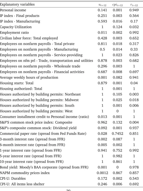
Tables C1 and C2 summarize the results for those predictor variables and own lags, respectively, that have the highest probabilities. Variables which had average posterior
probability less than0:5in all of the three equations are not included at all in the tables.
Each element in these tables is the BMA posterior probability and can be interpreted simply as the probability that the corresponding right-hand side variable should be in-cluded. For this specific application the variables are not orthogonalized in order to retain the interpretation of the probabilities as the amount of belief that the respective variable is included in the model. The results are based on 150,000 iterations with a burn-in period of 50,000, which leaves 100,000 draws to evaluate the posterior of . Elicitation of prior hyperparameters is based on the values described in Section 4.2.
Note that the probabilities !for are 0.52, 1, and 1 for each of the upper diagonal
elements 12, 13, and 23 respectively. Once all these probabilities are available, it is
straightforward to interpret them. This output can be used to implement BMA if all variables contribute to the final forecast according to their probability, no matter how high or low this probability is. Looking for example at Table C1, the spread of the 10-year interest rate from the federal funds rate variable will contribute to the final forecast of the unemployment rate, the consumer price index, and the interest rate in 100, 86.1, and 100%of the occasions (models visited by the sampler), respectively. In contrast the same output can be used to select the best single model. Barbieri and Berger (2004) show that in the context of Bayesian model selection the optimal model is the median probability model. According to this result, only the variables which have average probability larger than 0.5 in each equation will be unrestricted. These probabilities are presented in Tables C1 and C2. Hence, in this “best” model, the 1, 5, and 10-year interest rate spreads should be included in all three equations, while capacity utilization should enter only the unemployment equation.
4.4 Forecasting in Large VAR Models
The first estimation period is set to 1960:1 and a simulated real-time forecasting ofyt+h
is done from 1983:1 through 2003:12-h, for horizonsh= 1;6;and12. Each VAR model
has eight dependent variables of interest (with their short mnemonic from the dataset in
parentheses): Personal Income (A0M052), Industrial Production (IP S10), Employment
Rate (CES002), Unemployment Rate (LHU R), 3-month Treasury Bill Rate (F Y GM3),
Producer Price Index (P W F SA), Consumer Price Index (P U N EW), and PCE Deflator
(GM DC). This leaves a total of 124 variables to explore their predictive content. As mentioned earlier, all the variables are transformed to stationarity, a fact that implies
a specific transformation of the variableyt+h proper for forecasting. Let vit denote the
untransformed value of yit for each of the eight monthly dependent variables i, then
yit+h = (1200=h) log (vit+h=vit) for i = (A0M052; IP S10; CES002), yit+h = vit+h vit
for i = (LHU R; F Y GM3), and yit+h = (1200=h)flog (vit+h=vit) h log (vit)g for i =
(P W F SA; P U N EW; GM DC).
The principal components are estimated from the 124 variables in the dataset using the same sample period as the VAR. Several multivariate forecasting exercises in the literature (cf. Stock & Watson, 2002) focus on finding the best performing model. In contrast, here the main challenge is to improve forecasts when the number of predic-tors grows large and the researcher has no prior information about which is the correct model size. Thus, the maximum potential number of factors and lags is deliberately set
to large, “uninformative” values. In particular, 10 principal components (k = 10) are
extracted from the factor model in equation (2), while the VAR specification in
equa-tion (3) contains an intercept, 13 autoregressive lags (p1 = 12), and 13 lagged factors
(p2 = 12). This gives a maximum of 221 (plus the intercepts, which are unrestricted)
An appropriate common way to quantify out-of-sample forecasting performance is to compute the root mean square forecast error (RMSFE) statistic for each forecast horizon
h:
RM SF Eh ij =
v u u
t2003:12X h
t=1982:12
yi;t+h yei;t+h;j
2
(12)
where yi;t+h is the realized (observed) value ofy at time t+h for the i-th series, and
e
yi;t+h;j is the mean of the posterior predictive density at time t+h, for the i-th series,
from the j-th forecasting model. The RMSFE of each model is reported relative to the
RMSFE of a benchmark VAR with an intercept and seven lags of the dependent variables, estimated with OLS
rRM SF Eh ij =
RM SF Eh ij
RM SF Eh iV AR(7)
(13)
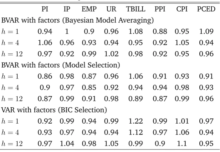
This VAR(7) model is not chosen because of its higher forecasting ability compared to other alternatives. Following the standard convention in the literature an AR(2) model would be a better candidate to serve as the benchmark model. But note that the VAR(7) is nested to the VAR with factors, which will give a better picture of whether the restrictions found by the SSVS are actually the ones that will lead to reduced RMSFE statistics, compared to a more parsimonious alternative. The forecasting performance
of the models based on the relative RMSFE for horizons h = 1;6;12, is summarized in
Table C3. These are the averaged values of the RMSFEs over the forecast period, 1983:1
through 2003:12-h.
zero, while Bayesian model selection imposes that these parameters (with probability less than 0.5) will be exactly zero.
5. CONCLUSIONS
This paper addresses the forecasting performance of Bayesian VAR models with many predictors using a flexible prior structure which leads to output that can be used for model selection and model averaging. For eight U.S. monthly macroeconomic variables of interest forecasting accuracy is improved over least squares estimation and selection of predictors using the Bayesian information criterion. Without arguing that the choice of prior hyperparameters was the best possible and done with a strict “objective” cri-terion (like in other BMA applications, see Fernandez et al., 2001), the gains from the standard automated choices are appreciable. As already mentioned, there are many proposals in the Bayesian literature for efficient elicitation of prior hyperparameters for model selection and some of them were discussed in the paper. Nevertheless, the merit of the SSVS for VAR models lies in its simplicity and intuitive interpretation.
ACKNOWLEDGMENTS
The author would like to thank Gary Koop and participants and discussants at several workshops and conferences for helpful comments. Part of this research was supported by the Department of Economics, University of Strathclyde, which I gratefully acknowl-edge.
REFERENCES
Andersson, M. K., & Karlsson, S. (2008). Bayesian forecast combination for VAR
mod-els. In: S. Chib, W. Griffiths, G. Koop & D. Terrell (Eds), Bayesian Econometrics
(pp. 501–524). Advances in Econometrics, Vol. 23. Oxford: Elsevier.
Banbura, M., Giannone, D., & Reichlin, L. (2007). Bayesian VARs with large panels. London: CEPR.
Barbieri, M. M., & Berger, J. O. (2004). Optimal predictive model selection. The Annals
of Statistics, 32, 870–897.
Bernanke, B. S., & Boivin, J. (2003). Monetary policy in a data-rich environment.
Journal of Monetary Economics, 50, 525–546.
Bernanke, B. S., Boivin, J., & Eliasz, P. (2005). Measuring the effects of monetary
policy: A factor-augmented vector autoregressive (FAVAR) approach. Quarterly
Journal of
Economics, 120, 387–422.
Brown, P. J., Vannucci, M., & Fearn, T. (1998). Multivariate Bayesian variable
selec-tion and predicselec-tion. Journal of the Royal Statistical Society. Series B (Statistical
Methodology), 60, 627–641.
Brown, P. J., Vannucci, M., & Fearn, T. (2002). Bayes model averaging with selection
of regressors. Journal of the Royal Statistical Society. Series B (Statistical
Method-ology), 64, 519–536.
Chipman, H., George, E. I., & McCulloch, R. E. (2001). The practical implementation
Lecture Notes –Monograph Series, Vol. 38. Beachwood, OH: Institute of Mathe-matical Statistics.
Favero, C. A., Marcellino, M., & Neglia, F. (2005). Principal components at work: The
empirical analysis of monetary policy with large datasets. Journal of Applied
Econometrics, 20, 603–620.
Fernandez, C., Ley, E., & Steel, M. (2001). Benchmark priors for Bayesian model
averaging. Journal of Econometrics, 100, 381–427.
George, E. I., & Foster, D. P. (2000). Calibration and empirical Bayes variable selection.
Biometrika, 87, 731–747.
George, E. I., & McCulloch, R. E. (1993). Variable selection via Gibbs sampling. Journal
of the American Statistical Association, 88, 881–889.
George, E. I., & McCulloch, R. E. (1997). Approaches to Bayesian variable selection.
Statistica Sinica, 7, 339–379.
George, E. I., Sun, D., & Ni, S. (2008). Bayesian stochastic search for VAR model
restrictions. Journal of Econometrics, 142, 553–580.
Gianone, D., Reichlin, L., & Sala, L. (2004). Monetary policy in real time (and
com-ments). In: M. Gertler & K. Rogoff (Eds),NBER Macroeconomics Annual 2004(pp.
161–224). Cambridge: The MIT Press.
Hoeting, J., Madigan, D., Raftery, A., & Volinsky, C. (1998). Bayesian model averaging:
A tutorial. Statistical Science, 14, 382–417.
Kadiyala, K. R., & Karlsson, S. (1997). Numerical methods for estimation and inference
in Bayesian VAR-models. Journal of Applied Econometrics, 12, 99–132.
Koop, G., & Potter, S. (2004). Forecasting in dynamic factor models using Bayesian
model averaging. Econometrics Journal, 7, 550–565.
Smith, M., & Kohn, R. (1996). Nonparametric regression using Bayesian variable
sec-tion. Journal of Econometrics, 75, 317–343.
Smith, M., & Kohn, R. (2002). Parsimonious covariance matrix estimation for
Stock, J. H., & Watson, M. W. (2002). Macroeconomic forecasting using diffusion
indexes. Journal of Business and Economic Statistics, 20, 147–162.
Stock, J. H., & Watson, M. W. (2003). Forecasting output and inflation: The role of
asset prices. Journal of Economic Literature, 41, 788–829.
Stock, J. H., & Watson, M. W. (2005a). Forecasting with many predictors. Unpublished Manuscript. Princeton University, Princeton, NJ (prepared for The Handbook of Economic Forecasting).
Stock, J. H., & Watson, M. W. (2005b). Implications of factor models for VAR analysis. Unpublished Manuscript. Princeton University, Princeton, NJ.
Strachan, R. W., & van Dijk, H. K. (2007). Bayesian model averaging in vector au-toregressive processes with an investigation of stability of the US great ratios and
risk of a liquidity trap in the USA, UK and Japan. Econometric Institute ReportEI
2007-11. Erasmus University Rotterdam, the Netherlands.
Yuan, M., & Lin, Y. (2005). Efficient empirical Bayes variable selection and estimation
APPENDICES
A
TECHNICAL APPENDIX – A GIBBS SAMPLER FOR SSVS
IN VAR MODELS
The priors described in Section 3 combined with the likelihood function of a VAR model, will allow us to derive and draw from the full conditional distributions. The likelihood
of the VAR modely=z +"," N(0; )with 1 = 0
, is
L(yj ; ) / j j T exp 1 2tr
0
(y z )0(y z )
= j j T exp 1
2 b
0
[ 0
(z0
z)] b 1
2tr y zb
0 0
y zb
where b is the MLE of . This form of the likelihood function allows to derive the
posterior of the parameters. In order to derive the posterior of the elements of
we need to first rewrite the likelihood function in convenient form. Define S( ) =
(y z )0
(y z ) and write S( ) = sij. For j = 2; :::; m define the (m 1) vectors
sj = s1j; :::; s(j 1)j
0
containing the upper diagonal elements of S( ), and the (m 1)
matricesSj containing the upper leftj j submatrix ofS( ). Define also 1 =s11 and
i = jSij=jSi 1j =sii s
0
iSi 11si for i = 2; :::; m. The likelihood function now cam take
the following form
L(yj ; )/ m
Y
i=1
( ii) T exp ( 1 2 " m X i=1 2
ii i+ m
X
j=2
j + jjSj11sj
0
Sj 1 j+ jjSj 11sj
#)
Now define D=diag h1; :::; hn' with
hi =
(
0i, if i = 0
1i, if i = 1
and, similarly, defineDj =diag h1j; :::; h(j 1)j with
hij =
(
0ij, if!ij = 0
1ij, if!ij = 1
fori= 1; :::; jandj = 2; :::; m. Then we can rewrite equations (6) and (10) in the main text, as
'kij N(0; DD) jj!j
iid
Nj 1(0; DjDj)
respectively. Denote the combined prior of the unrestricted coefficients 'c and the
re-stricted coefficients 'k as ' N '; V . Given starting values, model parameters are
drawn from their conditionals forr= 1; :::; Riterations:
1. Draw (r)j (r 1); !(r 1); (r 1); '(r 1); data by sampling each element from the
Gamma distribution
2
ii Gamma i+
1 2T; Bi
where
Bi =
(
1+12s11 fori= 1
i+12
h
sii s
0
i Si 1+ (DiDi) 1
1
si
i
fori= 2; :::; m
2. Draw (r)j (r)
; (r 1); '(r 1); !(r 1); data by sampling each element from the
Nor-mal distribution
j Nj 1 j; j
where forj = 2; :::; m.
j = jj Sj 1+ (DjDj) 1
1
sj j = Sj 1+ (DjDj) 1
1
distribution
(!ij) Bernoulli 1;
u1ij
u1ij +u2ij
where forj = 2; :::; mandi= 1; :::; j 1
u1ij =
1 0ij exp 2 ij 2 2 0ij ! qij
u2ij =
1 1ij exp 2 ij 2 2 1ij !
(1 qij)
4. Draw '(r)j (r); (r); !(r); (r 1); data by sampling ' = vec( ) from the Normal
distribution
(') Nnu( ; )
where
= ( 0
) (z0
z) +V 1 1 (( 0
) (z0
z))'b+V 1'
= ( 0
) (z0
z) +V 1 1
where 'b is the vector occuring from stacking the elements of the matrix of MLE
coefficients, i.e. b'=vec b =vec (z0
z) 1z0
y .
5. Draw (r)j (r); (r); !(r); '(r); data by sampling each element from the Bernoulli
density
( i) Bernoulli 1;
u1i
u1i+u2i
1. where for i= 1; :::; nu
u1i =
1 0i exp ' 2 i 2 2 0i pi
u2i =
1 1i exp ' 2 i 2 2 1i
B
DESCRIPTION OF DATA
This table lists the 132 variables in the dataset used. The third column indexes the respective transformation applied to each of the variables to ensure stationarity (at least approximately). Let vt and xt be the untransformed value and transformed values
respectively, then there are five cases:(1) lv: xt = vt (level), (2) ln: xt =log(vt)
(log-arithm), (3) lv: xt = vt vt 1 (first difference), (4) ln: xt = log (vt=vt 1) (growth
rate), and (5) 2ln: x
t = log (vt=vt 1):This table is from Stock and Watson (2005b)
and the reader should seek in this reference the original source of the data.
# Mnemonic Trans Description
1 A0M052 ln Personal income (ar, bil. chain 2000 $)
2 A0M051 ln Personal income less transfer payments (ar, bil.
chain 2000 $)
3 A0M224 ln Real consumption (A0M224=GM DC)
4 A0M057 ln Manufacturing and trade sales (mil. chain 1996 $)
5 A0M059 ln Sales of retail stores (mil. chain 2000 $)
6 IPS10 ln Industrial production index - total index
7 IPS11 ln Industrial production index - products, total
8 IPS299 ln Industrial production index - final products
9 IPS12 ln Industrial production index - consumer goods
10 IPS13 ln Industrial production index - durable consumer
goods
11 IPS18 ln Industrial production index - nondurable consumer
goods
12 IPS25 ln Industrial production index - business equipment
13 IPS32 ln Industrial production index - materials
14 IPS34 ln Industrial production index - durable goods
materi-als
15 IPS38 ln Industrial production index - nondurable goods
ma-terials
16 IPS43 ln Industrial production index - manufacturing17
17 IPS307 ln Industrial production index - residential utilities
18 IPS306 ln Industrial production index - fuels
# Mnemonic Trans Description
20 A0M082 lv Capacity utilization (mfg)
21 LHEL lv Index of help-wanted advertising in newspapers
(1967=100;sa)
22 LHELX lv Employment: ratio; help-wanted ads/ no.
unem-ployed clf
23 LHEM lv Civilian labor force: employed, total (thous.)
24 LHNAG lv Civilian labor force: employed, nonagricultural
in-dustries (thous.)
25 LHUR lv Unemployment rate: all workers, 16 years & over
(%)
26 LHU680 lv Unemployment by duration: average (mean)
dura-tion in weeks
27 LHU5 ln Unemployment by duration: persons unemployed
less than 5 wks (thous.)
28 LHU14 ln Unemployment by duration: persons unemployed 5
to 14 wks (thous.)
29 LHU15 ln Unemployment by duration: persons unemployed
15 wks + (thous.)
30 LHU26 ln Unemployment by duration: persons unemployed
15 to 26 wks (thous.)
31 LHU27 ln Unemployment by duration: persons unemployed
27 wks + (thous.)
32 A0M005 ln Average weekly initial claims, unemployment
insur-ance (thous.)
33 CES002 ln Employees on nonfarm payrolls - total private
34 CES003 ln Employees on nonfarm payrolls - goods-producing
35 CES006 ln Employees on nonfarm payrolls - mining
36 CES011 ln Employees on nonfarm payrolls - construction37
38 CES017 ln Employees on nonfarm payrolls - durable goods
39 CES033 ln Employees on nonfarm payrolls - nondurable goods
40 CES046 ln Employees on nonfarm payrolls - service-providing
41 CES048 ln Employees on nonfarm payrolls - trade,
# Mnemonic Trans Description
42 CES049 ln Employees on nonfarm payrolls - wholesale trade
43 CES053 ln Employees on nonfarm payrolls - retail trade
44 CES088 ln Employees on nonfarm payrolls - financial activities
45 CES140 ln Employees on nonfarm payrolls - government
46 A0M048 ln Employee hours in nonagricultural establishments
(ar, bil. hours)
47 CES151 lv Average weekly hours of production or
nonsupervi-sory workers on private nonfarm payrolls
48 CES155 lv Average weekly hours of production or
nonsupervi-sory workers on private nonfarm payrolls
49 AOM001 lv Average weekly hours: manufacturing (hours)
50 PMEMP lv NAPM employment index (percent)
51 HSFR ln Housing starts: nonfarm (1947-58); total farm
52 HSNE ln Housing starts: Northeast (thousands of units)
53 HSMW ln Housing starts: Midwest (thousands of units)
54 HSSOU ln Housing starts: South (thousands of units)55
56 HSBR ln Housing authorized: total new priv housing units
(thousands)
57 HSBNE ln Houses authorized by build. permits: Northeast
(thousands of units)
58 HSBMW ln Houses authorized by build. permits: Midwest
(thousands of units)
59 HSBSOU ln Houses authorized by build. permits: South
(thou-sands of units)
60 HSBWST ln Houses authorized by build. permits: West
(thou-sands of units)
61 PMI lv Purchasing managers’ index (sa)
62 PMNO lv NAPM new orders index (percent)
63 PMDEL lv NAPM vendor deliveries index (percent)
64 PMNV lv NAPM inventories index (percent)
65 A0M008 ln Mfrs’ new orders, consumer goods and materials
# Mnemonic Trans Description
66 A0M007 ln Mfrs’ new orders, durable goods industries (bil.
chain 2000 $)
67 A0M027 ln Mfrs’ new orders, nondefense capital goods (mil.
chain 1982 $)
68 A1M092 ln Mfrs’ unfilled orders, durable goods indus. (bil.
chain 2000 $)
69 A0M070 ln Manufacturing and trade inventories (bil. chain
2000 $)
70 A0M077 lv Ratio, mfg. and trade inventories to sales (based on
chain 2000 $)
71 FM1 2ln Money stock: M1 (bil$,sa)
72 FM2 2ln Money stock: M2 (bil$,sa)
73 FM3 2ln Money stock: M3 (bil$,sa)
74 FM2DQ ln Money supply - M2 in 1996 dollars (bci)
75 FMFBA 2ln Monetary base, adjusted for reserve requirement
changes(mil$,sa)
76 FMRRA 2ln Depository inst. reserves: total, adjusted for reserve
req changes (mil$,sa)
77 FMRNBA 2ln Depository inst. reserves: non-borrowed, adj
re-serve req changes (mil$,sa)
78 FCLNQ 2ln Commercial & industrial loans outstanding in 1996
dollars (bci)
79 FCLBMC lv Wkly rp lg com’l banks:net change com’l & indus
loans (bil$,saar)
80 CCINRV 2ln Consumer credit outstanding – non-revolving
81 A0M095 lv Ratio, consumer installment credit to personal
in-come (pct.)
82 FSPCOM ln S&P’s common stock price index: composite
(1941-43=10)
83 FSPIN ln S&P’s common stock price index: industrials
(1941-43=10)
84 FSDXP lv S&P’s composite common stock: dividend yield (%
# Mnemonic Trans Description
85 FSPXE ln S&P’s composite common stock: price-earnings
ra-tio (%)
86 FYFF lv Interest rate: Federal funds (effective) (% per
an-num)87
88 FYGM3 lv Interest rate: u.s. Treasury bills, sec market,
3-mo.(% per annum)
89 FYGM6 lv Interest rate: u.s. Treasury bills, sec market,
6-mo.(% per annum)
90 FYGT1 lv Interest rate: u.s. Treasury const maturities, 1-yr.(%
per annum)
91 FYGT5 lv Interest rate: u.s. Treasury const maturities, 5-yr.(%
per annum)
92 FYGT10 lv Interest rate: u.s. Treasury const maturities,
10-yr.(% per annum)
93 FYAAAC lv Bond yield: Moody’s AAA corporate (% per annum)
94 FYBAAC lv Bond yield: Moody’s BAA corporate (% per annum)
95 SCP90 lv CP90 – FYFF (spread)
96 SFYGM3 lv FYGM3 – FYFF (spread)
97 SFYGM6 lv FYGM6 – FYFF (spread)
98 SFYGT1 lv FYGT1 – FYFF (spread)
99 SFYGT5 lv FYGT5 – FYFF (spread)
100 SFYGT10 lv FYGT10 – FYFF (spread)
101 SFYAAAC lv FYAAAC – FYFF (spread)
102 SFYBAAC lv FYBAAC – FYFF (spread)
103 EXRUS ln United States; effective exchange rate (merm)
(in-dex no.)
104 EXRSW ln Foreign exchange rate: Switzerland (Swiss franc per
U.S.$)
105 EXRJAN ln Foreign exchange rate: Japan (yen per U.S.$)
106 EXRUK ln Foreign exchange rate: United Kingdom (cents per
pound)
107 EXRCAN ln Foreign exchange rate: Canada (Canadian$ per
# Mnemonic Trans Description
108 PWFSA 2ln Producer price index: finished goods (82=100,sa)
109 PWFCSA 2ln Producer price index: finished consumer goods
(82=100,sa)
110 PWIMSA 2ln Producer price index: intermed mat. supplies &
components (82=100,sa)
111 PWCMSA 2ln Producer price index: crude materials (82=100,sa)
112 PSCCOM 2ln Spot market price index: bls & crb: all
commodi-ties(1967=100)
113 PSM99Q 2ln Index of sensitive materials prices
(1990=100)(bci-99a)
114 PMCP lv NAPM commodity prices index (percent)
115 PUNEW 2ln CPI-u: all items (82-84=100,sa)116
117 PU84 2ln CPI-u: transportation (82-84=100,sa)
118 PU85 2ln CPI-u: medical care (82-84=100,sa)
119 PUC 2ln CPI-u: commodities (82-84=100,sa)
120 PUCD 2ln CPI-u: durables (82-84=100,sa)
121 PUS 2ln CPI-u: services (82-84=100,sa)
122 PUXF 2ln CPI-u: all items less food (82-84=100,sa)
123 PUXHS 2ln CPI-u: all items less shelter (82-84=100,sa)
124 PUXM 2ln CPI-u: all items less medical care (82-84=100,sa)
125 GMDC 2ln PCE, impl price deflator (1987=100)
126 GMDCD 2ln PCE, impl price deflator: Durables (1987=100)
127 GMDCN 2ln PCE, impl price deflator: Nondurables (1996=100)
128 GMDCS 2ln PCE, impl price deflator: Services (1987=100)
129 CES275 2ln Average hourly earnings of production or
nonsuper-visory workers on private nonfarm payrolls: goods
130 CES277 2ln Average hourly earnings of production or
nonsuper-visory workers on private nonfarm payrolls: con-struction
131 CES278 2ln Average hourly earnings of production or
nonsuper-visory workers on private nonfarm payrolls: manu-facturing
Table C1. Average Posterior Probabilities of Explanatory Variables in the 3-variable VAR
Explanatory variables ut+12 cpit+12 rt+12
Personal income 0.141 0.001 0.949
IP index - Final products 0.251 0.003 0.564
IP index - Manufacturing 0.593 0.016 0.17
Capacity Utilization 1 0.124 0.032
Employment ratio 0.011 0.002 0.992
Civilian labor force: Total employed 0.428 0.003 0.652
Employees on nonfarm payrolls - Total private 0.811 0.018 0.317
Employees on nonfarm payrolls - Manufacturing 0.5 0.014 0.33
Employees on nonfarm payrolls - Service-providing 1 0.023 0.826
Employees on nfm prl - Trade, transportation and utilities 0.878 0.003 0.682
Employees on nonfarm payrolls - Wholesale trade 0.296 0.003 1
Employees on nonfarm payrolls - Financial activities 0.687 0.008 0.697
Average weekly hours of production 0.001 0.082 0.941
Housing starts: Total 0.879 0.001 0.04
Housing authorized: Total 1 0.001 1
Houses authorized by building permits: Northeast 1 0.105 0.003
Houses authorized by building permits: Midwest 1 0.025 0.018
Houses authorized by building permits: South 1 0.001 0.006
Houses authorized by building permits: West 1 0 1
Consumer installment credit to Personal income (ratio) 0.013 0.001 1
S&P’S common stock price index: Composite 0.962 0.132 0.004
S&P’s composite common stock: Dividend yield 0.092 0.001 0.937
Commercial paper rate (spread from Fed Funds Rate) 0.028 0.7452 0.851
3-month interest rate (spread from FFR) 0.002 0.087 1
6-month interest rate (spread from FFR) 0.005 0.002 1
1-year interest rate (spread from FFR) 0.941 0.752 0.992
5-year interest rate (spread from FFR) 1 0.982 1
10-year interest rate (spread from FFR) 1 0.861 1
Bond yield: Moody’s BAA corporate (spread from FFR) 0.001 0 0.978
NAPM commodity prices index 0.0012 0.867 0.857
CPI-U: Durables 0.172 0.002 0.543
Table C2. Average Posterior Probabilities of AR-lags in the 3-variable VAR
Dependent Variable
Most important lags
(probability>0.5) Average posterior probability
ut+12 rt 7 0:56
cpit+12
rt 7
Own lags1to7(i.e. cpit tocpit 6)
cpit 7
0:74 1 0:83
rt+12 rt 6 1
Table C3. Forecast Comparison - relative RMSFE
PI IP EMP UR TBILL PPI CPI PCED
BVAR with factors (Bayesian Model Averaging)
h= 1 0.94 1 0.9 0.96 1.08 0.88 0.95 1.09
h= 4 1.06 0.96 0.93 0.94 0.95 0.92 1.05 0.94
h= 12 0.97 0.92 0.99 1.02 0.98 0.92 0.95 0.96 BVAR with factors (Model Selection)
h= 1 0.86 0.98 0.87 0.96 1.06 0.91 0.93 0.91
h= 4 0.9 0.97 0.85 0.92 0.94 0.94 0.98 0.93
h= 12 0.87 0.99 0.91 0.98 0.89 0.87 0.99 0.96 VAR with factors (BIC Selection)
h= 1 0.92 0.99 0.94 0.99 1.22 0.99 1.01 0.97
h= 4 0.93 0.97 0.94 0.94 1.12 0.97 1.06 0.94
h= 12 0.97 1.04 0.98 1.05 0.99 0.9 1.1 0.95 Note: The variables of interest are: PI: Personal Income (A0M052), IP: Industrial Production(IPS10), EMP:Employment Rate
(CES002), UR: Unemployment Rate (LHUR), TBILL: 3-month Treasury Bill Rate (FYGM3), PPI: Producer Price Index (PWFSA),
[image:31.595.125.477.309.552.2]