Consumer Survey Data and short-term
forecasting of households consumption
expenditures in Poland
Dudek, Sławomir
The Research Institute for Economic Development (RIED) - Warsaw
School of Economics (WSE)
August 2008
Online at
https://mpra.ub.uni-muenchen.de/19818/
Consumer Survey Data and short-term forecasting of
households consumption expenditures in Poland
Sławomir Dudek
The Research Institute for Economic Development (RIED)
The Warsaw School of Economics (WSE)
Abstract
The main aim of the paper is an investigation whether consumer tendency survey (CTS) data can be useful for short-term forecasting of real private consumption expenditures in Poland. A consumer sentiment index and as well balances for individual questions (from consumer survey conducted by Research Institute for Economic Development of Warsaw School of Economics – RIED WSE) were used in the paper. This is one of the first attempts to model private consumption using RIED consumer survey data or even generally any consumer survey data in Poland. The data are quarterly and covers the 1996-2007 period. An investigation of predictive relationship between CTS results and real private consumption was done by using in-sample and out-of-sample approach. Under the first one unconditional and conditional causality analysis was performed. Unconditional approach is a standard bivariate Granger causality test, where appropriate pairs of variables were tested: real private consumption expenditures and particular CTS indicators. In the case of conditional Granger causality test aside from consumer survey results other macro variables were used, i.e.: lagged dependent variable, real gross disposable income of households, net financial assets of households, retail sales and wage-pension fund. It was realized by doing redundancy tests for survey indices in ARMAX equation specified for consumption expenditures and other variables mentioned above. The research is also extended by assessing whether this predictive in-sample conditional relationship has changed over time by running a series of recursive regressions and doing tests outlined above. The out-of-sample analysis focused on testing recursive one-step forecast errors of restricted (without CTS variables) and unrestricted ARMAX models.
Key Words: consumption, consumer tendency survey, causality testing, comparing forecasts
1.
Introduction
The main aim of the paper is an investigation whether consumer tendency survey (CTS) data can be useful for short-term forecasting of real private consumption expenditures in Poland. A consumer sentiment indicator and as well balances for individual questions (from consumer survey conducted by Research Institute for Economic Development of Warsaw School of Economics – RIED WSE1) were used in the paper.
This is one of the first attempts to model private consumption using RIED (IRG) consumer survey data or even generally any consumer survey data in Poland (preliminary studies on that topic were performed in Białowolski and Dudek, 2008, 2005). In spite of variety of consumer surveys in Poland (currently 5 institutions are conducting the CTS2) there is no rich literature on application and usefulness of households attitudes and confidence on consumption in Polish economy. In general this issue is quite weakly examined in all new EU member states (NMS) in comparison with abundant literature for US, EU countries and other developed countries (in references there is only one position for NMS, i.e. for Hungary, Vadas, 2001). In the case of Poland generally private consumption behaviour (i.e. consumption function) is not sufficiently and in detail explored, in spite of its importance in generating GDP (more than 60%). Indeed there are few examples of estimated consumption function for Poland (see Fic et al., 2005; Viren et al., 2004). Mainly it is connected with a lack of necessary data and of course short samples. Quarterly national accounts (including consumption) starts since beginning of 1995, but private disposable income was not published for many years, CSO started to publish it in 2005 and time series starts since 1999. Quarterly net financial wealth of households is still not published. One also should be added that the mentioned time series were many times seriously revised (because of methodological changes).
As a macroeconomic database for Poland is developing there is an increasing possibility to study econometrically the factors influencing consumption growth. In the literature we can find many econometric work showing that measures of consumer confidence are highly correlated with changes of real consumption and may have some short-term forecasting ability. This big interest comes among others from the frequent reference to such measures in leading economic commentary and as well increasingly in policymaking. Similar situations is in Poland, publications of consumer survey results are very noticeable by media, are quite often commented by economist and policymakers. There is of course popular belief that consumer sentiment indicators are predicting consumption tendencies (and other macroeconomic variables as well).
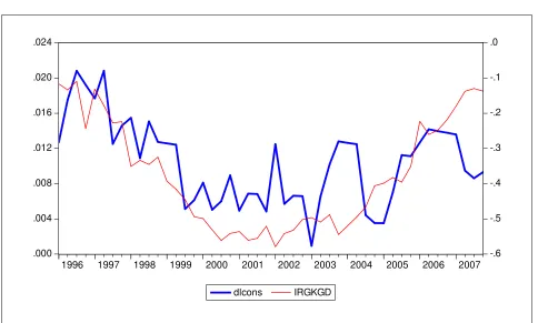
When we plot consumer sentiment indicator published by RIED against the log-change of consumption (Figure 1) we can see that there is some relationship and on the first look mentioned above belief is correct. However it have to be econometrically and statistically proved, what tend to be done further in this paper.
The paper was aimed among others to answer the several questions: Whether consumer sentiments are useful for predicting consumption in transitions countries (like Poland)? If so, which variable (question) are important? Is the relation between sentiments and consumption stable? Does it changed after EU accessions? Is the role of sentiments for consumption the same like in the developed countries or not?
1
Instytut Rozwoju Gospodarczego, Szkoła Główna Handlowa (IRG – SGH).
2
Figure 1 Consumer sentiment index (IRGKGD) and log-change of real private consumption
.000 .004 .008 .012 .016 .020 .024
-.6 -.5 -.4 -.3 -.2 -.1 .0
1996 1997 1998 1999 2000 2001 2002 2003 2004 2005 2006 2007
dlcons IRGKGD
Source: RIED WSE (IRG SGH), CSO (GUS).
2.
Background
Consumer tendency surveys have very long history. The first consumer confidence measures were devised in the late 1940’s by George Katona at the University of Michigan. The Michigan’s Consumer Sentiment Index is regularly published since the beginning of 1950’s to the present. As Richard Curtin (director of Surveys of Consumers at University of Michigan) stated in the paper on the occasion of the fiftieth birthday of the Michigan’s index “Consumer confidence is now one of the most closely watched indicators of future economic trends. The latest figures on sentiment trends are routinely reported in the press, and incorporated into many macroeconomic forecast models ….” (Curtin, 2000, p. 6). This sentence is also truth for other countries, the Consumer Tendency Surveys very soon achieved popularity all over the World, they are currently carried out in at least forty-five countries (Malgarini and Margani, 2005). In spite of very long history of CTS, the questions: “What is consumer confidence?”, “Why consumer sentiment may influence consumption behavior?”. “What is determining consumer confidence?” are still open.
Katona (1975) underlined that there could exist psychological factors besides the economic ones. Katona suggests that consumption behaviour of the household can be affected by two factors. The first one, specified as an objective, is related to the “traditional” economic fundamentals and was called by Katona as an “ability to buy”. The second one, seen rather as a subjective, is what Katona called “the willingness to buy”. While “ability to buy” depends on the financial resources of households and consumption prices (i.e. their budget constraint), the subjective factor may influence consumption in a more complex way. According to this approach consumption can be influenced by non-quantitative, non-economic factors - such as political crisis, elections or wars – supposed to have an impact on agent’s psychological mood. As a consequence the “willingness to buy” may be an important and independent explanatory factor for spending, especially for discretionary purchases (in particular, durable goods), and near to business cycle turning points. The “willingness to buy” is exactly what the consumer sentiment index tries to capture. In the presence of uncertainty, confidence indices could also capture desire for precautionary saving.
So as a result “… a rise in the confidence indicator implies an improvement in the expectations of future personal and general situation and/or a decrease in the degree of consumers’ subjective uncertainty, which should induce an increase in consumption” (Parigi and Schlitzer, 1995).
According to Desroches and Gosselin (2002) in general the empirical results in literature on predictive power of CTS indicators for consumption (as well other economic phenomenon’s) can be divided into three groups: (i) the indicators are of negligible value because they lose their explanatory power with the addition of control (macroeconomic) variables; (ii) they have an incremental explanatory value, since they contain information over and above that held in the controls; or (iii) they are useful because they improve forecasts of consumption growth (as well other economic phenomenon’s) during exceptional periods. Garner (1991) concludes that these diverging results are attributable to three factors:
• The information set differs between studies. Some studies link consumption to confidence and to only one or two variables, whereas others consider a broader set of control variables.
• The lag structure and the forecasting horizon are different. Some focus on a contemporaneous relationship between the variables, whereas others give much more importance to the dynamic effect of explanatory variables.
• The sample period is different. Since confidence appears to be especially useful to forecast consumption during extraordinary periods, the likelihood of concluding that confidence indexes are helpful is greater when such periods are covered.
So far, the literature on predictive power of CTS showed mixed conclusion, the usefulness of confidence indicators is not an obviousness. The mixed role of CTS’s is not only the issues of empirical factors outlined by Garner, this role also depends on institutional and behavioral aspects, and can be different in particular countries, regions, time spans, group of households, etc. It means that relaying on CTS results in the process of formulating opinions (by media, economist, policymakers) abut tendencies in consumption (or GDP) need to be econometrically and statistically grounded. So when there is started in some country new CTS it cannot be assumed automatically by analogy that it will allow for better predicting of consumption (GDP).
3.
General methodology
as the Campbell and Mankiw model).This approach often relays on in-sample testing of specially specified consumption equation.
The second approach is more empirical and is concentrating on testing out-of-sample forecasting properties of CTS indicators. This approach can be in addition narrowed to real-time data forecasting. The out-of-sample approach have to take into account the theoretical issues, but is constrained on availability, coverage and timeliness of data, especially real-time data. In practice it is not possible to reproduce full theoretical specification in forecasting models.
In this paper the analysis is concentrated on real-time forecasting (similar approach was used among others in Croushor, 2005; Slacalek, 2004). Out-of-sample analysis was used in Bovi, 2004, Easaw and Heravi, 2004, Howrey, 2001, Bram and Ludvigson, 1998. However it should be emphasized that here in the paper it is not full “real-time” approach because it takes into account only differences in publication time of particular set of data. Real-time data should also consider revisions in the data (such approach is used in Croushor, 2005). It is very important aspect, unfortunately in Poland doesn’t exist any publicly available real-time database with consecutive vintages of macro time series (like e.g. “Real-Time Data Set” in Federal Reserve Bank of Philadelphia3) and on other side it could be quite difficult to decide how to treat big methodological changes.
Basing on the work presented in the references the analysis in the paper is divided on several stages. In the first, preliminary stage, statistical analysis is performed, that is time series are tested on presence of unit roots. Investigation of predictive power of CTS indicators is divided on two blocks: in-sample analysis and out-of-in-sample analysis (both on real-time data).
Here should be mentioned again that in the paper predictive power is tested not only for consumer sentiment index but also for individual questions from harmonized questionnaire. Most of papers on that topic are focused on synthetic consumer sentiment index, but there is quite a lot analysis operating on question level, eventually on sub-indicies (see for example Slacalek, 2006; Bovi, 2004; Goh, 2003; Vadas, 2001; Bram and Ludvigson, 1998; Côté and Johnson, 1998; Batchelor and Dua, 1998, Berg and Bergstrom, 1996).
In the first block unconditional and conditional causality approach (following Al-Eyd et al., 2008) is used as well as correlation analysis on whole available sample (1996:Q1-2007Q4). Unconditional approach is a standard bivariate Granger causality test, where appropriate pairs of variables were tested: real private consumption growth and CTS indicators. In the case of conditional Granger causality test aside from consumer survey results other macro variables were used, i.e.: lagged dependent variable, real gross disposable income of households, net financial assets of households, retail sales and wage-pension fund. It was realized by doing redundancy tests for survey indices in ARMAX equation specified for consumption expenditures and other variables mentioned above. Conditional causality framework is the most used approach on that issues in the literature. See for example Acemoglu and Scott (1994), Carroll et al. (1994), Bram and Ludvigson (1998), Côté and Johnson (1998), Loundes and Scutella’s (2000), Vadas (2001), Desroches and Gosselin (2002), Goh (2003), Sommer (2003), Jansen and Nahuis (2004), Bovi (2004), Slacalek (2004), Malgarini and Margani (2005), Croushore (2005) and Al-Eyd et al. (2008). What is important conditional causality approach in this paper is based on real-time data. The research is also extended by assessing whether this predictive in-sample relationships has changed over time by running a series of recursive regressions (over the period 2003:Q1-2007:Q4) and doing tests outlined above.
The main idea of the out-of-sample analysis is to compare forecasts obtained from the models including CTS indicators with forecast received from models without this variables. To quantify this
3
Data bank for US economy is available at web page:
comparison two kind of tests are used: test for equality of mean squared errors and test for forecasts encompassing.
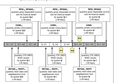
[image:7.595.65.534.258.599.2]As was stated above this paper deal with real-time forecasting. So described above methodological approach have to take into account availability of all time series in the moment of doing forecast or in the moment of testing conditional Granger causality. On the Figure 2 there is presented publication and forecasting schedule of real private consumption and its potential explanatory indicators including CTS indictors. From the diagram we can read what are a publication delays for CTS indicators, private consumption and other macroeconomic variables (i.e. real private disposable income - RPDI, real net assets - RFINAS, real retail sales - RETSEL and real wage and pension fund - RWPF4) used further in the analysis.
Figure 2 Publication and forecasting schedule of real private consumption and potential explanatory indicators
CONS-2
quarterly private consumption for quarter Q-2
[+60 days]
RPDI-2, RFINAS-2
quarterly gross disposable income and net financial wealth
for quarter Q-2 [+90 days]
quarterly CTS (RIED WSE) results
for quarter Q [-55 days]
RETSEL-2, RWPF-2
quarterly retail sales and wage&pension fund
for quarter Q-2 [+20 days]
quarterly CTS (RIED WSE) results for quarter Q+1
[-55 days] CONS-1
quarterly private consumption for quarter Q-1
[+60 days]
RPDI-1, RFINAS-1
quarterly gross disposable income and net financial wealth
for quarter Q-1 [+90 days]
CONS
quarterly private consumption for quarter Q
[+60 days] RPDI, RFINAS
quarterly gross disposable income and net financial wealth
for quarter Q [+90 days]
Q-1, m1 Q-1, m2 Q-1, m3 Q, m1 Q, m2 Q, m3 Q+1, m1 Q+1, m2 Q+1, m3
RETSEL-1, RWPF-1
quarterly retail sales and wage&pension fund
for quarter Q-1 [+20 days]
RETSEL, RWPF quarterly retail sales and
wage&pension fund for quarter Q
[+20 days] quarterly CTS (RIED
WSE) results for quarter Q-1 [-55 days]
Remarks: Q, Q-1, Q+1 – current, previous, next quarter; m1, m2, m3 – first, second and third month of the quarter; [+dd] – number of days from the end of reporting quarter (publication delay), in the case of CTS variable it is negative because survey is conducted during the first month of the surveyed quarter.
As we can see from the diagram CTS quarterly results are published very early, the survey is conducted during the first month of the surveyed quarter, so the results are published on the beginning of second month, i.e. 55 days before the end of reporting period. So in spite of some theoretical, behavioural aspects we can advantage also from publication time. Consumption (and all main
4
quarterly national accounts) is published 60 days after reporting quarter. This mean that in the moment when CTS are available we don’t even posses data on reference variable for previous quarter. Unfortunately in Poland quarterly income accounts (including private disposal income) are published quite late, 90 days after reporting quarter. Data about quarterly households assets are not yet publicly available. There are available some elements of assets and researchers try to calculate aggregate assets series themselves (see Zachłod-Jelec, 2008). This is very big problem in general for modelling consumption in Poland, practically it prevent researches from using standard consumption function in real time. Also it should be underlined that very often, households aggregate income and financial wealth are used as a control variables in testing predictive power of CTS indicators, especially income. In real-time approach we have to consider publications lags for that control variables. The problem with availability of control variable of consumption could be to some extent overcome by using high frequency data on retail sales and wage and pension fund, which are published very early, i.e. 20 days after reporting quarter (month).
On the scheme there are also indicated the moments where forecasts of real private consumptions will be performed in this study. The reference period of predictive power testing is current quarter (Q) for which forecast of consumption will be made. From this point of view we should treat this exercise to some extent as a nowcasting. There are defined 3 forecasting moments which in the context of real-time-data are determining possible sets of explanatory variables5:
• F1 – 30 days before the end of reference quarter,
• F2 – end of the reference quarter,
• F3 – 20 days after reference quarter.
So, finally in the econometric analysis many models were used which specification (composition) is a combination of moments of performing forecast (or testing), set of macroeconomic (control) variables and particular CTS indicator.
4.
Preliminary statistical analysis – unit root tests
As a preliminary step the time series on stationarity are examined. It is natural stage in all econometric analyses. But in this paper for stationarity issues there is devoted a little bit more attention than in usual econometric analyses. It is connected with quite ambiguous results in that field for CTS variables, which tend to be “near unit root” series (as called by Golinelli and Parigi, 2003, 10) or “near random walk” series.
On the beginning we should note that consumer tendency survey indicators are by definition a “bounded series”. They are defined as balances of positive and negative structure indictors, so by construction their values are fluctuating between minus 100 and plus 100 percentage points, in other words its are mean reverting series. Also it should be noted that the most of questions in consumer survey concern households opinions about changes of particular economic phenomenon’s. Numerous econometric analyses are showing that changes (growth rates) of most of economic time series are stationary. This two factors means that CTS indicators cannot trend over time, although it may within a finite, short subsample. As was also suggested by Al-Eyd et al.: “Heuristically speaking, confidence cannot determine consumption in the long run, since people cannot go on being excessively (un) confident forever, as by construction confidence is a relative measure, and we might expect it to be stationary.” (Al-Eyd et al., 2008, p. 2).
The problem of presence of unit roots in the CTS time series in some papers is more deeply investigated. See for example Bovi (2004), where two test together are performed for Italian CTS
5
indicators (sample: 1982-2003). The author received mixed results finally interpreting CTS indicators as stationary. Bovi summarized this results saying that “… it is hard to think about an everlasting “irrational exuberance (or apprehension)” in all agents.”. Other interesting example is a paper quite substantially devoted to the stationarity problem of US and UK consumer sentiment indicators, Easaw and Ghoshray (2002). The authors using ADF test concluded that CSI for US is non-stationary but for UK CSI is non-stationary (sample: 1978-2001). On other hand they found out that CSI for US has asymmetric cyclical nature (aspirations are downwardly rigid). They underlined that the ADF test assumes a symmetric adjustment process and as a consequence is not a relevant one in this situation. Using unit root test assuming asymmetric adjustment (TAR and M-TAR model) they concluded that CSI for US is stationary.
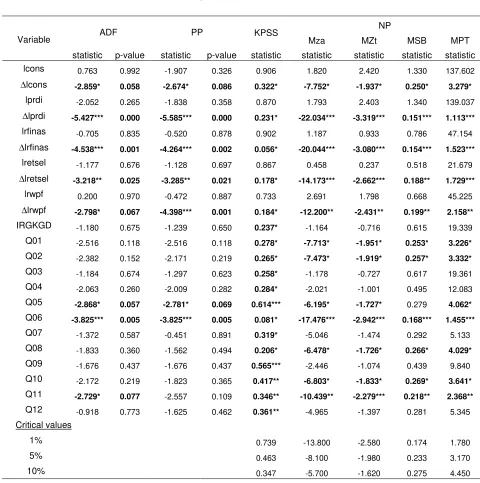
This research is based on quite short sample (48 observations). It is well known that unit root tests are based on asymptotic critical values and some of them are known to have low power against the alternative hypothesis that the series is stationary for finite samples. To overcome slightly this problem several unit root tests were performed: Augmented Dickey-Fuller test (ADF), Phillips-Perron test (PP), Kwiatkowski-Phillips-Schmidt-Shin test (KPSS) and Ng-Perron test (NP). The ADF and PP test are most popular unit root test in the literature, but in finite short samples this test posses very low power. The use of NP test yields both, substantial power gains and a lower size distortions over the standard unit root tests, maintaining the null of unit root. The KPSS test can be thought as complementing one because it tests the null hypothesis of stationarity, just the opposite to the previous one. The results of unit root tests are presented in Table 1. Additionally graphs of all series used in analysis are presented in appendix 2 (Figures 3 and 4).
Unit root tests for macroeconomic time series are in line with general consensus. Natural logarithms of real private consumption, real private disposable income, real net assets, real retail sales and real wage and pension fund are generated by process I(1). All four test are implying this conclusion.
Unfortunately, as it was occurring in other papers, for consumer survey indicators results are very mixed. In general ADF test is showing non-stationarity for the most of indicators. Only for 3 qualitative indicators (out of 13 analysed) stationarity was proved. Two indicators are near-stationary (p-value 11-15%). According to Ng-Perron test statistics 7 qualitative indicators are stationary. On other side KPSS test is indicating stationarity of all consumer survey indicators. Ambiguous unit root test results are to big extent connected with very short sample of available data. To some extent it could be also explained by the fact that analysed sample covers the period of transition of Polish economy from centrally (undeveloped) one to the market economy. During this period rapid convergence process occurred and as well as we had numerous institutional and structural changes. As a result majority of economic time series could behave as trending one or they are disturbed by some structural changes. Taking this results into account and also results and conclusions form other papers (and countries) in the next parts of the analysis macroeconomic (control) variables will be used in first differences where as consumer tendency survey indicators in levels.
Table 1 Unit root tests (sample: 1996:Q1-2007Q4)
NP
ADF PP KPSS
Mza MZt MSB MPT
Variable
statistic p-value statistic p-value statistic statistic statistic statistic statistic
lcons 0.763 0.992 -1.907 0.326 0.906 1.820 2.420 1.330 137.602
∆lcons -2.859* 0.058 -2.674* 0.086 0.322* -7.752* -1.937* 0.250* 3.279*
lprdi -2.052 0.265 -1.838 0.358 0.870 1.793 2.403 1.340 139.037
∆lprdi -5.427*** 0.000 -5.585*** 0.000 0.231* -22.034*** -3.319*** 0.151*** 1.113***
lrfinas -0.705 0.835 -0.520 0.878 0.902 1.187 0.933 0.786 47.154
∆lrfinas -4.538*** 0.001 -4.264*** 0.002 0.056* -20.044*** -3.080*** 0.154*** 1.523***
lretsel -1.177 0.676 -1.128 0.697 0.867 0.458 0.237 0.518 21.679
∆lretsel -3.218** 0.025 -3.285** 0.021 0.178* -14.173*** -2.662*** 0.188** 1.729***
lrwpf 0.200 0.970 -0.472 0.887 0.733 2.691 1.798 0.668 45.225
∆lrwpf -2.798* 0.067 -4.398*** 0.001 0.184* -12.200** -2.431** 0.199** 2.158**
IRGKGD -1.180 0.675 -1.239 0.650 0.237* -1.164 -0.716 0.615 19.339
Q01 -2.516 0.118 -2.516 0.118 0.278* -7.713* -1.951* 0.253* 3.226* Q02 -2.382 0.152 -2.171 0.219 0.265* -7.473* -1.919* 0.257* 3.332* Q03 -1.184 0.674 -1.297 0.623 0.258* -1.178 -0.727 0.617 19.361 Q04 -2.063 0.260 -2.009 0.282 0.284* -2.021 -1.001 0.495 12.083 Q05 -2.868* 0.057 -2.781* 0.069 0.614*** -6.195* -1.727* 0.279 4.062* Q06 -3.825*** 0.005 -3.825*** 0.005 0.081* -17.476*** -2.942*** 0.168*** 1.455*** Q07 -1.372 0.587 -0.451 0.891 0.319* -5.046 -1.474 0.292 5.133 Q08 -1.833 0.360 -1.562 0.494 0.206* -6.478* -1.726* 0.266* 4.029* Q09 -1.676 0.437 -1.676 0.437 0.565*** -2.446 -1.074 0.439 9.840 Q10 -2.172 0.219 -1.823 0.365 0.417** -6.803* -1.833* 0.269* 3.641* Q11 -2.729* 0.077 -2.557 0.109 0.346** -10.439** -2.279*** 0.218** 2.368** Q12 -0.918 0.773 -1.625 0.462 0.361** -4.965 -1.397 0.281 5.345 Critical values
1% 0.739 -13.800 -2.580 0.174 1.780 5% 0.463 -8.100 -1.980 0.233 3.170 10% 0.347 -5.700 -1.620 0.275 4.450 a) ADF - Augmented Dickey-Fuller test with constant term, lag length selected using SIC; PP - Phillips-Perron test
with constant term, bandwidth selected using Newey-West with Bartlett kernel; KPSS - Kwiatkowski-Phillips-Schmidt-Shin test with constant term, bandwidth selected using Newey-West with Bartlett kernel; NP - Ng-Perron test with constant term (four statistics Mzα, Mzt, MSB i MPT), lag length selected using SIC with spectral GLS-detrended AR estimation.
b) Bold values imply stationarity (with at least 10%), it implies rejection of null of unit root or the non rejection of the null hypothesis of stationarity (in the KPSS case); *) critical value at 10%, **) 5%, ***) 1%.
c) ∆… – first difference, l… – natural logarithm.
and aggregate sentiment indexes are either stationary or borderline stationary, in analysis he used all CTS indicators in levels. Jansen and Nahuis (2004) for time span (1985-1998) proved stationarity of CSI for Belgium, Germany, France, Italy, Netherlands, Portugal, Spain and UK; thus in estimation all CTS variables were used in levels. Hardouvelis and Thomakos (2007) in their paper analyzed sentiment indicators for 14 of EU15 countries (1985-2005). The ADF test rejected the null hypothesis of a unit root in only 6 among the 14 countries. Authors also found out the presence of long memory in all consumer sentiment indexes. They decided that all series are best characterized as being stationary but having strong long memory. They argued that the ADF test has documented low power and can easily “confuse” a highly persistent stationary series with a non-stationary series having a unit root.
On other hand Gelper et al. (2007) using ADF test found out Michigan sentiment index to be non-stationary (1978-2004) and they are using in modelling consumption CSI in differences. Jansen and Nahuis (2003) using ADF and PP tests for CSI’s for 11 EU countries (1986-2001) also found unit roots and in modelling they used differences of sentiment indicators, but what is strange this result is in opposition to their paper cited above It might be connected with longer sample. Opposite results to the cited above (Bovi, 2004) for Italian consumer survey were obtained by Malgarini and Margani (2005). This authors concluded that ISAE Consumer Confidence is characterized by the presence of a unit root and therefore first-differencing the series seems to be the more appropriate, they used sample 1980-2004.
Combination of above conclusions is quite confusing, especially when opposite results were received for the same consumer surveys (the same country). But we have to remember that majority of practical applications for consumption growth forecasting use CTS indicators in levels. Quite sporadic analyses are based on differences of CTS indicators. These cases should be rather treated as statistical relationships in chosen sample, because it is quite difficult to explain theoretically, modeling in long-term of trending (no mean reverting) series (i.e. consumption) by mean reverting (maybe with some persistence) series, i.e. CTS indicators.
5.
Unconditional and conditional Granger causality test (in-sample
analysis)
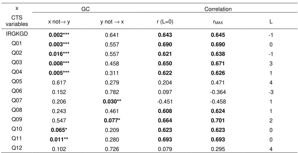
In the preliminary stage of the research correlations analysis and standard bivariate Granger Causality test (for specification see e.g. EViews 6 User’s Guide I, 2007, p. 411) were performed. Pairs of log-change of real private consumption and CTS indicators were subject of analysis. It was conducted over whole available sample (1996-2007). The results are presented in Table 2, which contains p-values for F-statistic of redundancy test. In the column denoted with “x not → y” there are estimations of the probability that a CTS variable is not a cause – in Granger`s sense - of the log-change of private consumption. In the column “y not → x” you may find probabilities that the log-change of private consumption is not a cause of CTS variable. In table there are also showed contemporaneous and maximum cross correlation coefficients.
In general correlation analysis is showing strong positive correlation of CTS indicators with log-change of private consumption in Poland. For 9 CTS indicators (out of 13) contemporaneous correlation coefficients are higher than 0,6 (it ranged from 0.608 to 0.693). Weak correlation was received only for inflation assessments (Q05 and Q06) and current financial standing (Q12). For unemployment expectations results are showing negative correlation (Q07).
(Q02-Q04) and savings expectations (Q11). Other two CTS indicators, current climate for savings (Q10) and current financial standing (Q12) pass GC test with 10% p-value.
What is interesting the balance concerning expectations about unemployment (Q07) which is according to EU methodology a component of sentiment index, is not useful for predicting change of consumption, there is even opposite results, reverse causality. Assessments of present and future major purchases (Q08, Q09) are highly correlated with log-change of consumption but are not causing reference variable (for Q09 we received even reverse causality). Correlation and GC analysis is showing that present and future assessment of inflation are not useful for explaining consumption development.
[image:12.595.54.535.317.564.2]Summing up preliminary analysis it could be stated that in Poland CTS indicators could be useful for predicting changes in real private consumption. Especially if we take into account assessments of (current and expected) personal financial situation of household and general situation of total economy.
Table 2 Bivariate Granger causality, contemporaneous and cross correlation coefficients of ∆∆∆∆lcons with CTS variables (sample: 1996:Q1-2007:Q4)
GC Correlation
x
CTS
variables x not→ y y not → x r (L=0) rMAX L
IRGKGD 0.002*** 0.641 0.643 0.645 -1
Q01 0.003*** 0.557 0.690 0.690 0
Q02 0.016*** 0.557 0.621 0.638 -1
Q03 0.008*** 0.458 0.650 0.671 3
Q04 0.005*** 0.311 0.622 0.626 1
Q05 0.617 0.279 0.204 0.471 4
Q06 0.152 0.782 0.097 -0.364 -3
Q07 0.206 0.030** -0.451 -0.458 1
Q08 0.243 0.461 0.608 0.624 1
Q09 0.547 0.077* 0.664 0.701 2
Q10 0.065* 0.209 0.623 0.623 0
Q11 0.011** 0.280 0.693 0.693 0
Q12 0.102 0.726 0.079 0.295 4
a) y – ∆lcons; GC – granger causality test, x not → y – empirical level of p-value (F-test) for the hypothesis that x is not a cause of y in Granger`s sense; y not → x – empirical level of p-value (F-test) for the hypothesis that y is not a cause of x in Granger`s sense. Bold values imply significance with at least 10%, *) critical value at 10%, **) 5%, ***) 1%.
b) 4 lags were used for each variable in specification of Granger causality test and 4 leads/lags for cross-correlation analysis.
But above approach is unconditional and excludes the possible influence of other variables on the reference variable. It is not a proof that consumer attitudes and sentiments are direct and behavioural factors which affect consumption. They can just reflect development of other macro variables.
indices in equation specified for consumption expenditures and other variables mentioned above. General testing specification is based on very standard and popular approach in literature of such kind of analysis, starting with paper of Carroll et al. (1994). Her in the paper there is used slightly modified specification, which takes into account publication delay of macroeconomic variables, what means that it takes into account real-time data. Quite similar specifications for forecasting of GDP using general economic sentiment index (ESI) was proposed in Gelper and Croux (2007). In the forecasting (testing) equation on the left hand side we have log-difference of real private consumption which is explained by own lags and distributed lags of CTS variables and macro variables:
t i
k i t k i
m i
m p i t m i i
i t i
t
const
lcons
Z
Q
lcons
=
+
α
∆
+
β
m+
δ
+
ε
∆
∑
∑ ∑
∑
= −
∈ = −−
= −
4
0 4
0 4
1 MACRO
(1)
Such model is specific form of the most general, dynamic single equation specification, that is ARMAX (Franses, 1991 or Bierens, 1987), called also as a ARMADL (Davidson, 2000). In equation (1)
m t
Z
stands for log-differences of macroeconomic variables,p
m is a publication delay for that variables, this delay depends on variable and moment of making forecast (F1, F2 or F3). In the equation there are used different sets of macro variables out of mentioned above,{
lrpdi
lrfinas
lretsel
lrwpf
}
MACRO
m
∈
=
∆
,
∆
,
∆
,
∆
. For all moments of forecasts, current CTSindicators are available thus in specification publication lag is omitted for
Q
tk (p
k=
0
),{
IRGKGD
,
Q
01
,
Q
02
,
,
Q
12
}
CTS
k
∈
=
. Taking into account theoretical and practical reasons(especially publication schedule) in the analysis have been used 11 sets of macro variables, 5 sets for F1 forecasts, 3 sets for F2, and 2 sets for F3 forecasts. In all specifications 4 lags of dependent variables were included (AR(4)) and of course CTS variables (one in each specifications). The sets are:
1. F1a – specification without macro variables (only AR(4)),
2. F1b – specification with
∆
lretsel
−1to−4,3. F1c - specification with
∆
lrwpf
−1to−4,4. F1d - specification with
∆
lrpdi
−2to−5,5. F1e - specification with
∆
lrfinas
−2to−5,6. F1f - specification with
∆
lrpdi
−2to−5,∆
lrfinas
−2to−5,7. F2a - specification with
∆
lrpdi
−1to−4,8. F2b - specification with
∆
lrfinas
−1to−4,9. F3c - specification with
∆
lrpdi
−1to−4,∆
lrfinas
−1to−4,10. F2a – specification with
∆
lretsel
0to−4,Composition of defined above sets of macroeconomic variables is based on theoretical and practical grounds. Real private disposable income and real net financial assets of households (sets: F1d, F1e, F1f, F2a, F2b, F2c) are chosen due to their presence in typical consumption functions. This variables are also most often included in equations for testing conditional predictive power o CTS indicators. Motivations for inclusion to above sets of retail sales index and pension and wage fund are rather practical (sets: F1b, F1c, F3a, F3b). Both variables are fast, high-frequency indicators, very often used by economist and analyst in Poland to assess changes of private consumption. The retail sales is a proxy of consumption development from the supply side. Real wage and pension fund is the first proxy of aggregate households income, so its use is theoretically grounded, but it should be noted that it cover only part of total personal income.
Conditional Granger causality test is performed by redundancy test on all lags of CTS indicator in equation (1) with all possible sets of macro variables defined above. Formally it is tested zero restriction on estimated parameters for particular CTS variable separately:
0
,
0
,
0
,
0
,
0
1 2 3 40
=
=
=
=
=
k k
k k
k
β
β
β
β
β
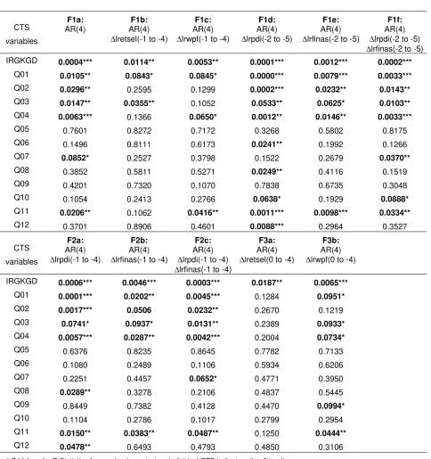
. F-statistic is used. The testing equations are estimated forwhole available sample (1996-2007). The results for all CTS indicators and all sets of macro variables are presented in Table 3, for simplicity only p-values associated with F-statistic are shown. P-values smaller than 5% (or eventually 10%) for particular specification (set of conditional variables) indicate that adding macro variable/s do not exclude CTS indicators from information set useful for forecasting of consumption.
Bearing in mind quite good results for simple bivariate Granger causality test and correlation analysis here we find some notable differences. For the equations allowing the earliest forecast for current quarter (set F1: 30 days before the end of the quarter) results are showing that inclusion of the change in the log of retail sales and real wage and pension fund separately (F1b and F1c) excludes most of CTS indicators which have been significant in simple bivariate Granger causality test case (for 5% significance level). In both cases (F1b and F1c) consumer sentiment index (IRGKGD) is still significant. With that models also assessment of general economic situation (Q3) is not excluded. For lagged real wage and pension fund only expectations on savings (Q11) can not be excluded with 5% significance level. If we take into account 10% significance level also assessment of current personal financial situation (Q01) could help in predicting consumption.
Conditional Granger causality test for equations with two-quarter lagged real personal income and net financial wealth (F1d, F1e, F1f) doesn’t change conclusions from simple bivariate GC test. It means that CTS indicators have extra explanatory power over information included in real personal income and net financial wealth. The same conclusion is drawn when we are analysing equations used for forecasting at the moment F2 with that set of macro variables (F2a, F2b and F2c). Additional observations on quarter Q-1 for real personal income and financial wealth doesn’t reduce predictive power of CTS indicators. To some extent it is quite surprising result because this mean that real private income (RPDI) has less information content for predicting consumption than real wage and pension fund (RWPF), which represent less than 60% of households income.
Substantial differences have been received for equation used for forecasting at the moment F3 (F3a and F3b). In the specification with retail sales with observations up to the current quarter (nowcasting case) only sentiment index (IRGKGD) is not excluded. In the case of real wage and pension fund (F3b) additional observations on current quarter in comparison with specification F1c doesn’t change very much the conclusions. CTS indictors Q01, Q03, Q04, Q09 have additional predictive power, but only with 10% significance level. Sentiment index and question on future saving (Q11) are significant with 5%.
and pension fund are reducing a role of CTS, especially the first one. Only consumer sentiment index emerged from conditional GC test unscathed for all possible configuration of macro variables.
Table 3 Conditional Granger causality test for CTS indicators with different equation specifications (sample: 1996:Q1-2007:Q4)
CTS
variables
F1a:
AR(4)
F1b:
AR(4)
∆lretsel(-1 to -4)
F1c:
AR(4)
∆lrwpf(-1 to -4)
F1d:
AR(4)
∆lrpdi(-2 to -5)
F1e:
AR(4)
∆lrfinas(-2 to -5)
F1f:
AR(4)
∆lrpdi(-2 to -5)
∆lrfinas(-2 to -5)
IRGKGD 0.0004*** 0.0114** 0.0053** 0.0001*** 0.0012*** 0.0002***
Q01 0.0105** 0.0843* 0.0845* 0.0000*** 0.0079*** 0.0033***
Q02 0.0296** 0.2595 0.1299 0.0002*** 0.0232** 0.0143**
Q03 0.0147** 0.0355** 0.1052 0.0533** 0.0625* 0.0103**
Q04 0.0063*** 0.1366 0.0650* 0.0012** 0.0146** 0.0033***
Q05 0.7601 0.8272 0.7172 0.3268 0.5802 0.8175
Q06 0.1496 0.8111 0.6173 0.0241** 0.1992 0.1266
Q07 0.0852* 0.2527 0.3798 0.1522 0.2679 0.0370**
Q08 0.3852 0.5811 0.5271 0.0249** 0.4116 0.1519
Q09 0.4201 0.7320 0.1070 0.7838 0.6735 0.3048
Q10 0.1054 0.2413 0.2766 0.0638* 0.1929 0.0888*
Q11 0.0206** 0.1062 0.0416** 0.0011*** 0.0098*** 0.0334**
Q12 0.3701 0.8906 0.4601 0.0088*** 0.2964 0.3527
CTS
variables
F2a:
AR(4)
∆lrpdi(-1 to -4)
F2b:
AR(4)
∆lrfinas(-1 to -4)
F2c:
AR(4)
∆lrpdi(-1 to -4)
∆lrfinas(-1 to -4)
F3a:
AR(4)
∆lretsel(0 to -4)
F3b:
AR(4)
∆lrwpf(0 to -4)
IRGKGD 0.0006*** 0.0046*** 0.0003*** 0.0187** 0.0065***
Q01 0.0001*** 0.0202** 0.0045*** 0.1284 0.0951*
Q02 0.0017*** 0.0506 0.0232** 0.2670 0.1219
Q03 0.0741* 0.0937* 0.0131** 0.2389 0.0933*
Q04 0.0057*** 0.0287** 0.0042*** 0.2004 0.0734*
Q05 0.6376 0.8235 0.8645 0.7782 0.7133
Q06 0.1080 0.2489 0.1106 0.5934 0.6206
Q07 0.2251 0.4457 0.0652* 0.4771 0.3950
Q08 0.0289** 0.3278 0.2106 0.4837 0.5445
Q09 0.8449 0.7382 0.4128 0.4470 0.0994*
Q10 0.1104 0.2786 0.1017 0.2799 0.2954
Q11 0.0150** 0.0383** 0.0487** 0.1250 0.0444**
Q12 0.0478** 0.6493 0.4793 0.4850 0.3106
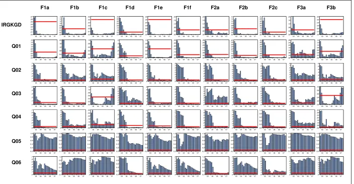
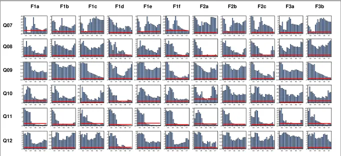
In the next step the research was also extended by assessing whether this predictive, in-sample relationships has changed over time. It is performed by running a series of recursive regressions and doing conditional Granger causality tests outlined above. The starting sample was set to 1997:Q1-2002:Q4, then recursively estimation sample was extended forward step-by-step by one quarter. For each recursion conditional Granger causality test was performed in the same manner like above. The results are presented in appendix 2. Figure 5a and 5b plots over time (2003-2007) p-values from recursive redundancy test. As above -values smaller than 5% for particular specification (set of conditional variables) indicate that adding macro variable/s do not exclude CTS indicators.
For sentiment index (IRGKGD) and balances concerning present and future personal financial situation, general economic situation (Q01-Q04) and savings expectations (Q11) we can observe decreasing tendency of significance level for all specifications. For some equations on the beginning of recursive sample (2003-2004), conditional GC test is even suggesting exclusion of that CTS variables. It means that predictive power of these CTS indicators is increasing in time, especially after 2004 when Poland acceded to European Union. But this results should be to some extend interpreted quite carefully because of short starting estimation sample and thus low number of degrees of freedom. The recursive test in general rather confirmed that balances concerning current and future inflation, expected unemployment, major purchases, current savings climate and present financial standing (Q05-Q10, Q11-Q12) don’t possess predictive power over set of macroeconomic variables used in analysis. For that CTS indicators p-values in almost all equations and all recursive periods are above 5% level.
6.
Predictive power of CTS indicators (out-of-sample analysis)
The main idea of this stage of analysis is to compare the out-of-sample forecasts obtained from the restricted and the unrestricted models (with CTS indicator). Restricted model means that we exclude from the equation (1) indicators from the consumer survey
Q
tk.For out-of-sample analysis purposes from the sample there were excluded last P=20 observations, it covers period 2003:Q1-2007:Q4. Thus the starting estimation sample include R=24 observations (if we take into account 4 lags in models specification), it covers period 1997:Q1-2002:Q4. Using defined above models (equation 1) in unrestricted and restricted form, 20 point forecasts were calculated recursively with re-estimation of that models. At each recursion the estimation sample was increased by one quarter forward and forecasted point (quarter) also. For all models there were calculated forecast errors and average measures like root mean squared error (RMSE) and mean squared error (MSE).
In order to formally investigate whether the forecasts from unrestricted regression model are significantly superior to the forecasts from restricted one, there were used: the Theil’s ratio (called in some papers as a U statistic), the McCracken (2004) MSE-F and Clark and McCracken (2001) ENC-NEW statistics.
Theil’s U statistic is defined as the ratio of the square roots of the mean squared forecasting errors (RMSE) of the unrestricted model and the restricted one. If Theil’s U statistic is smaller than one, then the forecasts based on the CTS indicators are superior to the forecasts of the restricted models.
good size properties and are typically more powerful than the original statistics in extensive Monte Carlo simulations with nested models.
The MSE-F statistic is used to test the null hypothesis that the unrestricted model forecast mean squared error (MSE) is equal to the restricted model forecast MSE against the one sided (upper-tail) alternative hypothesis that the unrestricted model forecast MSE is less than the restricted model forecast MSE. A significant MSE-F statistics indicates that the unrestricted model forecasts are statistically superior to those of the restricted model. In other words it means that CTS indicators have additional predictive power for modelling consumption (they reduce forecasting error). Clark and McCracken (2005) demonstrated that the MSE-F statistics shares a non-standard limiting distribution. Critical values fort that test are taken from Clark and McCracken tables (2001)6.
The second out-of-sample statistic, ENC-NEW, relates the concept of forecast encompassing. Forecast encompassing is based on optimally constructed composite forecasts. Intuitively, if the forecasts from the restricted regression model encompass the unrestricted model forecasts, the CTS variables included in the unrestricted model provides no useful additional information for predicting change of real consumption relative to the restrictive model which excludes the CTS variables. If the restricted model forecasts do not encompass the unrestricted model forecasts, then the CTS indicators do contain information useful for predicting change of real consumption beyond the information already contained in a model that excludes the CTS variables. In general forecast encompassing tests consist in testing whether the weight attached to the unrestricted model forecast is zero in an optimal composite forecast composed of the restricted and unrestricted model forecast. In the Clark and McCracken ENC-NEW test under the null hypothesis the weight attached to the unrestricted model forecast in the optimal composite forecast is zero, and the restricted model forecasts encompass the unrestricted model forecasts. Under the one sided (upper tail) alternative hypothesis, the weight attached to the unrestricted model forecast in the optimal composite forecast is greater than zero so that the restricted model forecasts do not encompass the unrestricted model forecasts. Similarly to the case of the MSE-F statistics, the limiting distribution of the ENC-NEW statistic is non-standard and pivotal when comparing forecasts from nested models. Critical values fort that test are taken from Clark and McCracken tables (2001).
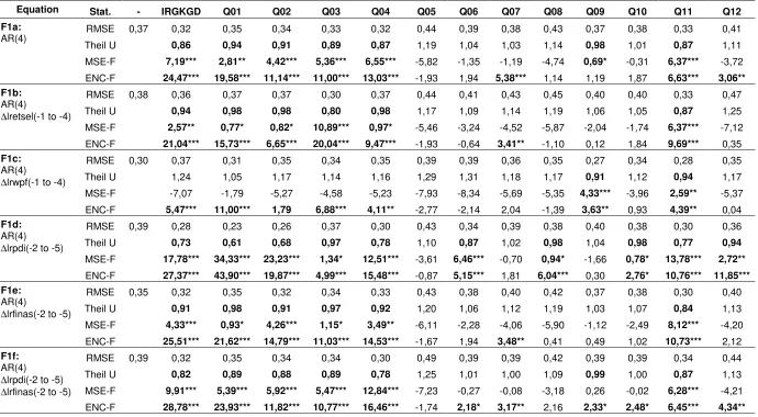
The results of out-of-sample analysis are presented in Tables 4a and 4b for particular CTS indicators, as well for different sets of macro variables (specifications).
Out-of-sample analysis to large extent confirmed good predictive power of CTS indicators explored in the previous stage of analysis. The results are even much better in the context of usefulness of CTS for consumption forecasting. Again consumer sentiment index (IRGKGD) and balances concerning present and future personal financial situation and general economic situation (Q01-Q04) and savings expectations (Q11) give additional predictive power. For all specifications F1 with that indicators, forecasts from unrestricted model are superior to the forecasts from restricted specifications (see Table 4a). In all cases RMSE is smaller (Theil U ratio is smaller than 1) and this differences are significant according to Clark-McCracken MSE-F test. In addition the forecast from restricted models are not encompassing forecasts from unrestricted one with that CTS variables, what is indicated by ENC-F test. For the rest CTS indicators in specifications F1 in most cases (with exception of model F1d for Q06, Q08, Q10, Q12 and F1c for Q09) RMSE’s are higher in unrestricted models. What is interesting forecasts from models (F1a, Fi1b, F1e, F1f) with unemployment expectations (Q07) in spite of higher forecasting error are not encompassed by restricted ones.
6
Equation Stat. - IRGKGD Q01 Q02 Q03 Q04 Q05 Q06 Q07 Q08 Q09 Q10 Q11 Q12
RMSE 0,37 0,32 0,35 0,34 0,33 0,32 0,44 0,39 0,38 0,43 0,37 0,38 0,33 0,41
Theil U 0,86 0,94 0,91 0,89 0,87 1,19 1,04 1,03 1,14 0,98 1,01 0,87 1,11
MSE-F 7,19*** 2,81** 4,42*** 5,36*** 6,55*** -5,82 -1,35 -1,19 -4,74 0,69* -0,31 6,37*** -3,72
F1a:
AR(4)
ENC-F 24,47*** 19,58*** 11,14*** 11,00*** 13,03*** -1,93 1,94 5,38*** 1,14 1,19 1,87 6,63*** 3,06**
RMSE 0,38 0,36 0,37 0,37 0,30 0,37 0,44 0,41 0,43 0,45 0,40 0,40 0,33 0,47
Theil U 0,94 0,98 0,98 0,80 0,98 1,17 1,09 1,14 1,19 1,06 1,05 0,87 1,25
MSE-F 2,57** 0,77* 0,82* 10,89*** 0,97* -5,46 -3,24 -4,52 -5,87 -2,04 -1,74 6,37*** -7,12
F1b:
AR(4)
∆lretsel(-1 to -4)
ENC-F 21,04*** 15,73*** 6,65*** 20,04*** 9,47*** -1,93 -0,64 3,41** -1,10 0,12 1,84 9,69*** 0,35
RMSE 0,30 0,37 0,31 0,35 0,34 0,35 0,39 0,39 0,36 0,35 0,27 0,34 0,28 0,35
Theil U 1,24 1,05 1,17 1,14 1,16 1,29 1,31 1,18 1,17 0,91 1,12 0,94 1,17
MSE-F -7,07 -1,79 -5,27 -4,58 -5,23 -7,93 -8,34 -5,69 -5,35 4,33*** -3,96 2,59** -5,37
F1c:
AR(4)
∆lrwpf(-1 to -4)
ENC-F 5,47*** 11,00*** 1,79 6,88*** 4,11** -2,77 -2,14 2,04 -1,39 3,63** 0,93 4,39** 0,04
RMSE 0,39 0,28 0,23 0,26 0,37 0,30 0,43 0,34 0,39 0,38 0,40 0,38 0,30 0,36
Theil U 0,73 0,61 0,68 0,97 0,78 1,10 0,87 1,02 0,98 1,04 0,98 0,77 0,94
MSE-F 17,78*** 34,33*** 23,23*** 1,34* 12,51*** -3,61 6,46*** -0,70 0,94* -1,66 0,78* 13,78*** 2,72**
F1d:
AR(4)
∆lrpdi(-2 to -5)
ENC-F 27,37*** 43,90*** 19,87*** 4,99*** 15,48*** -0,87 5,15*** 1,81 6,04*** 0,30 2,76* 10,76*** 11,85***
RMSE 0,35 0,32 0,35 0,32 0,34 0,33 0,43 0,38 0,40 0,42 0,37 0,38 0,30 0,40
Theil U 0,91 0,98 0,91 0,97 0,92 1,20 1,06 1,12 1,19 1,03 1,07 0,84 1,13
MSE-F 4,33*** 0,93* 4,26*** 1,15* 3,49** -6,11 -2,28 -4,06 -5,90 -1,12 -2,49 8,12*** -4,20
F1e:
AR(4)
∆lrfinas(-2 to -5)
ENC-F 25,51*** 21,62*** 14,79*** 11,03*** 14,53*** -1,67 1,94 3,48** 0,41 0,49 1,02 10,73*** 2,12
RMSE 0,39 0,32 0,35 0,34 0,34 0,30 0,49 0,39 0,39 0,42 0,39 0,39 0,34 0,44
Theil U 0,82 0,89 0,88 0,89 0,78 1,25 1,01 1,00 1,09 0,99 1,00 0,87 1,13
MSE-F 9,91*** 5,39*** 5,92*** 5,47*** 12,84*** -7,23 -0,27 -0,08 -3,18 0,26 -0,02 6,28*** -4,21
F1f:
AR(4)
∆lrpdi(-2 to -5)
∆lrfinas(-2 to -5)
ENC-F 28,78*** 23,93*** 11,82*** 10,77*** 16,46*** -1,74 2,18* 3,17** 2,16 2,33* 2,48* 6,45*** 4,34**
a) Presented RMSE’s are multiplied by 100, so its can be interpreted approximately as a percentage points of growth rate. Theil U coefficient is defined as a ratio of RMSE of unrestricted model over restricted one.
[image:18.842.90.780.89.469.2]Equation Stat. - IRGKGD Q01 Q02 Q03 Q04 Q05 Q06 Q07 Q08 Q09 Q10 Q11 Q12
RMSE 0,46 0,34 0,30 0,33 0,45 0,35 0,50 0,44 0,44 0,42 0,51 0,45 0,41 0,41
Theil U 0,74 0,65 0,72 0,98 0,76 1,09 0,95 0,96 0,91 1,11 0,97 0,90 0,89
MSE-F 16,48*** 28,05*** 19,04*** 0,74* 14,71*** -3,31 2,11** 1,71* 4,06** -3,88 1,27* 4,80*** 5,27***
F2a:
AR(4)
∆lrpdi(-1 to -4)
ENC-F 24,61*** 29,43*** 14,24*** 3,55** 12,58*** -0,98 2,54* 2,14 5,70*** -1,05 2,18* 3,91** 7,18***
RMSE 0,34 0,32 0,32 0,32 0,34 0,32 0,43 0,37 0,39 0,39 0,36 0,37 0,31 0,40
Theil U 0,94 0,93 0,93 1,00 0,92 1,25 1,07 1,15 1,13 1,06 1,08 0,90 1,17
MSE-F 2,46** 2,95** 3,03** 0,03 3,73** -7,18 -2,51 -4,88 -4,45 -2,26 -2,69 4,73*** -5,47
F2b:
AR(4)
∆lrfinas(-1 to -4)
ENC-F 21,19*** 21,13*** 10,35*** 7,12*** 10,84*** -2,34 1,31 2,27* 1,47 -0,28 0,58 6,96*** 1,76
RMSE 0,40 0,31 0,35 0,36 0,34 0,31 0,50 0,39 0,39 0,43 0,43 0,40 0,37 0,46
Theil U 0,78 0,87 0,88 0,85 0,77 1,22 0,96 0,97 1,06 1,06 0,98 0,91 1,12
MSE-F 13,10*** 6,24*** 5,95*** 7,64*** 14,10*** -6,63 1,92** 1,30* -2,26 -2,03 0,84* 4,26*** -4,19
F2c:
AR(4)
∆lrpdi(-1 to -4)
∆lrfinas(-1 to -4)
ENC-F 26,93*** 16,72*** 8,83*** 8,68*** 13,17*** -1,66 3,14** 4,40** 2,09 0,16 2,44* 4,76** 0,91
RMSE 0,33 0,35 0,34 0,33 0,30 0,31 0,37 0,35 0,42 0,38 0,38 0,35 0,29 0,38
Theil U 1,06 1,01 0,98 0,91 0,95 1,11 1,06 1,26 1,14 1,14 1,07 0,89 1,14
MSE-F -2,34 -0,51 0,64* 4,25*** 2,33** -3,62 -2,19 -7,38 -4,61 -4,55 -2,52 5,49*** -4,62
F3a:
AR(4)
∆lretsel(0 to -4)
ENC-F 15,58*** 13,63*** 6,22*** 14,36*** 8,25*** -1,23 -0,03 1,27 -0,59 1,58 1,71 12,06*** -0,33
RMSE 0,31 0,37 0,32 0,35 0,36 0,35 0,41 0,42 0,36 0,36 0,28 0,35 0,28 0,35
Theil U 1,22 1,04 1,14 1,19 1,15 1,33 1,36 1,18 1,17 0,92 1,13 0,93 1,13
MSE-F -6,65 -1,40 -4,54 -5,85 -4,91 -8,63 -9,17 -5,67 -5,28 3,60** -4,28 3,22** -4,43
F3b:
AR(4)
∆lrwpf(0 to -4)
ENC-F 4,99*** 10,97*** 2,50* 4,96*** 4,47** -2,92 -2,39 1,95 -1,41 3,67** 0,29 5,13*** 0,00
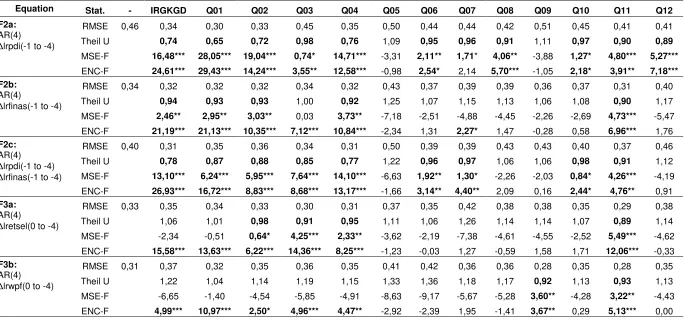
a) Presented RMSE’s are multiplied by 100, so its can be interpreted approximately as a percentage points of growth rate. Theil U coefficient is defined as a ratio of RMSE of unrestricted model over restricted one.
[image:19.842.93.777.89.411.2](Q11). In the most cases for that variables forecasting errors are significantly lower in unrestricted model. Exceptions are models F3a with IRGKGD and Q01 and models F3b for all mentioned here variables. But forecasts from that models are not encompassed (see ENS-F test) by forecasts received without CTS variables. It means that consumer survey indicators do contain information useful for predicting change of real consumption beyond the information already contained in a model that excludes the CTS variables. For the rest CTS indicators results are ambiguous, in general they don’t have predictive additional power over macro economic variables but in some cases they do (for model F2a and F2c).
Quite interesting is comparison of predictive power of different forecasting models by the moment of running it. Surprisingly moving from F1 moment (2/3 of forecasted quarter) through F2 (the end of forecasted quarter) to F3 moment (20 days after reporting quarter) in general doesn’t reduce average forecasting error. The smallest forecasting errors have been received for model F1d (RPDI) with sentiment index and Q01 and Q02 balances. However it wasn’t formally tested.
From this comparison we can also conclude that the use of CTS indicators together with some other macroeconomic variables give more precise forecasts than using CTS indicators alone (F1a model).
7.
Conclusions
The paper was aimed to answers the several questions: Whether consumer sentiments are useful for predicting consumption in transitions countries (like Poland)? If so, which indicator (question) is important? Is the relation between sentiments and consumption stable? Does it changed after EU accessions? Is the role of sentiments for consumption the same like in the developed countries or not?
The achieved results showed that some of CTS indicators in Poland have predictive power for forecasting of real private consumption growth. What is important the predictive power was not reduced after inclusions to the forecasting models other macroeconomic variables (i.e. real private disposable income, real net financial assets, retail sales index or real wage and pension fund). So they contain important additional information not contained in the economic variables typically included in the consumption regressions. The results are quite robust to using various statistical procedures (in-sample and out-of (in-sample approach; unconditional and conditional Granger causality test).
Taking into account lack of such analysis for other Eastern European countries it’s difficult to expand conclusion of strong predictive power generally for transition EE countries. Good predictive power of CTS indicators was received also for Hungary (see Vadas, 2001).