A Non destructive Defect Estimation Method for Metal Pole Based on Machine Learning Approach

A Non-destructive Defect Estimation Method for Metal Pole

Based on Machine Learning Approach

Shuji Takahashi

_{, Masaya Miyajima}

_{, Atsushi Horiguchi}

_{, Kyoji Nakajo}

_,

Kazuhiro Motegi

_{, Yochi Shiraishi}

_{and Takashi Suda}

1_{AZAPA Co., LTD., 2-4-15 Nishiki, Naka-ku, Nagoya, Aichi 460-0003, Japan}

2_{Department of Mechanical Science and Technology, Graduate School, Gunma University, 29-1}

Honcho, Ohta, Gunma 373-0057, Japan

3_{Yoshimoto Pole Co., Ltd., 508 Naka-Kurisu, Fujioka, Gunma 375-0015, Japan}

4_{Gunma Industrial Technology Center, 884-1 Kamesato-cho, Maebashi, Gunma 379-2147, Japan}

*[email protected] *Corresponding author

Keywords: Non-destructive testing, Defect estimation, Machine learning, Support vector machine, Hammering sounds, FFT, Metal pole.

Abstract.

This paper suggests a non-destructive defect estimation method for metal

pole by analyzing its hammering sounds. A machine learning algorithm, that is,

Support Vector Machine algorithm is applied for the spectrum distributions obtained

from the hammering sounds by using a Fourier Transform. A defect estimation

algorithm incorporating this algorithm is actually developed and tested for 200

hammering sounds of metal poles with/without a defect. The number of hammering

sounds used for the learning phase is 180 and the remaining 20 are used for test

phase. As a result, 100% accuracy rate is attained and this shows the feasibility of

machine learning approach.

Introduction

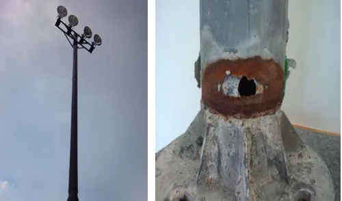
A serious physical or property accident is caused when a defected large metal pole which is used as a brace member for traffic signal or lighting pole falls over. The left photo in Fig.1 shows the actual lighting pole whose height is around eight meters and it has a lighting device on top of it. The devices are various kinds of lighting equipments, traffic signals, road signposts or speakers, etc. The right photo shows an example of defects and this is a hole with rusted area around the land surface. At present, the specialists visually check such defects periodically, however, there is a possibility that they fail to find such defects.

Conventionally, the testing methods using such means as radioactive ray, ultrasonic wave, magnetic particles, liquid penetration, eddy-current, visual observation and acoustic emission, are suggested. Each of the means has merits and demerits and the authors selected the acoustic emission approach because the inspection device using this method is simple, compact and, then, not expensive. Moreover, the authors have experiences in this approach [1]. The non-destructive defect estimation by analyzing hammering sounds forms an active research field and, actually, much effort has been devoted to estimate, for example, the defects in concrete constructions [2][3][4]. A typical approach is to firstly apply an FFT (Fast Fourier Transform) or a Wavelet Transform to the hammering sounds and then to visualize the results in the two or three dimensional graphical images. Next, the researchers must find the characteristics whichcan be used for defect estimation by visually analyzing the obtained images. Actually, the authors suggested a defect estimation method for metal poles by extracting some frequencies representing the characteristics in the FFT spectrum distributions [5]. However, afterwards, it is noticed that the approach to make a judgement standard in such way is not necessarily applicable when the target metal poles are changed or the sound recording method is modified.

In the 2010’s, in the machine learning field, some algorithms [6] attract much attention from the application view and it is said that the third great progress may be expected in the AI research. The authors select the Support Vector Machine (SVM) [7][8] as a machine learning algorithm for extracting the characteristics in the FFT distribution. The SVM algorithm is implemented by using a MATLAB function [9] and it is trained by using 180 from 200 sound data generated by hammering 500mm metal pole samples, where 100 sound data are with a defect and 100 sound data are without a defect. Then, it is tested to the remaining 20 ones and the result shows the 100% accuracy rate.

Non-destructive Defect Estimation by Hammering Sounds

In the non-destructive defect estimation, there are two phases, one is to devise a judgement standard and another is to test the object based on the judgement standard. The former is an important problem and this problem is to be solved in this paper. The goal in this problem-solving is shown in Fig.2. In the conventional approaches [1][2][3][4], only the procedures shown in the real space are executed.

Figure 2. Goal of Non-destructive Defect Estimation.

the generated judgement standard. Therefore, in the virtual space in Fig.2, the same non-destructive defect estimation is executed. Actually, the models of the tested metal pole and the hammer are constructed and the hammering and analyzing processes are executed. In this case, the modal analysis based on the Finite Element Method [10] is applied. Under some restricted conditions, a judgement standard is devised by this approach [5]. However, when the hammer is improved in order to reduce the dispersion of hammering sounds and moreover, the metal pole is changed, the judgement standard devised before cannot be valid.

Defect Estimation Method Based on Machine Learning Algorithm

In order to devise a new judgement standard, the authors adopt a machine learning algorithm. Support Vector Machine Algorithm

The Support Vector Machine (SVM) algorithm is efficient for dividing a given set of data into basically two subsets based on their characteristics [7][8]. The SVM algorithm can generate a hyperplane, called a support vector, separating two subsets in order to maximize the distance between the divided two subsets. Here, ∈ is a d-dimensional real vector and ∈ 1, 1 is the attribute of (i = 1, …, n).

Training Data: , | ∈ , ∈ 1, 1 . (1)

Hyperplane: y x/s W b. (2)

The output of SVM algorithm is the above hyperplane, where the parameters are weight vector, ∈ , the scale parameter, s and the bias parameter, ∈ . In the application of SVM

algorithm in this paper, the d-dimensional real vectors, , ∈ and the attribute correspond to the spectrum distribution of hammering sounds and the healthy (-1) or defected (+1) status, respectively.

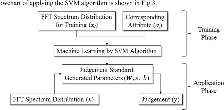
Implementation of SVM Algorithm by Using MATLAB The flowchart of applying the SVM algorithm is shown in Fig.3.

Figure 3. Flowchart of SVM Algorithm Application.

In the Application Phase, the FFT distribution, ∈ which should be judged is the input and its score y is calculated by using the expression (2) with the above parameters. Finally, y is used for

judging healthy or defected.

Experimental Results

Metal Pole Samples

The samples shown in Fig.4 are cut from an actual eight meter long metal pole. The metal pole is made from STK400 (99.5% steel) [11] according to the JIS (Japan Industrial Standard) G 3444. The dimensions are 500mm height, 165mm diameter, 5mm thickness, 9kg weight and the Young ratio and the Poisson ratio are 206GPa and 0.30, respectively. The sample (b) has a hole with 30mm φ.

Figure 4. Metal Pole Samples used in Experiments.

Training in SVM algorithm

The number of spectrum distributions is 200 and they are FFT-transformed from the hammering sounds. The number of sounds adopted from the healthy and the defected metal poles are equally 100. These hammering sounds are recorded with the 44.1kHz sampling frequency and the 16b sampling rate. The dimensions of spectrum distribution is 22050, that is, ∈ (i = 1, …,

200). In the training phase, 180 training data are randomly selected and they are consisting of 90 healthy and 90 defected. After the training phase, the set of parameters shown in Table 1 is obtained.

The SVM algorithm gives an appropriate weight to each of the spectrum and calculates the score

y which can be used for separating the given set. On the other hand, the visual observation only

concentrates on the several peaks of spectrums based on, for example, the modal analysis [5][10]. This difference between the SVM algorithm and the visual observation may cause the difference of accuracies of judgement standard. The CPU time for this training is about five minutes.

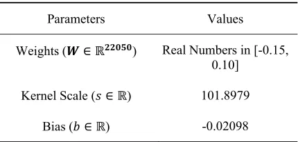
Table 1. Parameter Values obtained as a Result of Training.

Parameters Values

Weights ( ∈ ) Real Numbers in [-0.15, 0.10]

Kernel Scale ( ∈ ) 101.8979

Bias ( ∈ ) -0.02098

Test and Evaluation

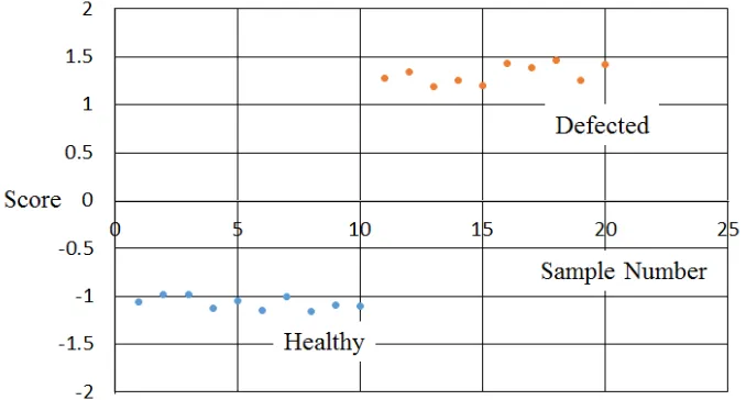
The set of 20 spectrum distributions consisting of 10 healthy and 10 defected samples are used for evaluating the performance of judgement standard. The score calculation is based on the expression (2) and the parameters shown in Table 1 are used. The judgement standard is shown below.

Score Calculation: y /101.8979 0.02098.

Judgement Standard: y ≧ 1 ∶

respectively. The healthy samples are numbered from 1 to 10 and the defected samples are from 11 to 20. Each of the scores is less than or around -1 or greater than +1 and the accuracy ratio in judgement attains 100%.

Figure 5.Test Result.

Conclusions and Future Work

The judgement standard is constructed by the Support Vector Machine (SVM) algorithm. The spectrum distributions obtained by applying the Fourier Transform to the hammering sounds are used in the estimation. In the experiments, 100% accuracy ratio is attained and the suggested method can be used for the practical use. As future work, this method should be applied to the actual eight meter long metal poles first and then, to various types of metal poles.

References

[1] Yoichi Shiraishi, Yuuki Okada and Kozo Yoshizawa, “A Defect Estimation Method within a Trunk Based on Wavelet Analysis by Diagnostic Slapping Sounds,” Journal of Japan Forest Society, vol. 90, no. 4, pp. 223-231, 2008.

[2] Y. Sonoda and K. Kawabe, “A Fundamental Study on Diagnosis Performance of Hammering Test using FE Acoustics Analysis,” 35th Conference on Our World in Concrete & Structures, pp. 25-27, 2010.

[3] Yutaka Manabe, Tsukasa Abe and Akio Iwase, “Basic Study on Non-Destructive Test for Cracks and Peel-offs of Concrete,” Research Reports of Hokuriku Branch, Architectural Institute of Japan, no. 43, pp. 219-222, 2000.

[4] Mariko Yamasaki, Yasuo Doi and Yasutoshi Sasaki, “Nondestructive Inspection for Member of Timber Structure using Stress Wave Velocity - Part 1 Bending Rigidity Prediction of Wood Beam with a Notch,” Summaries of Technical Papers of Annual Meeting, no. 43, pp. 373-374, 2009.

[5] Shuji Takahashi, Keitaro Mizunuma, Atsushi Horiguchi, Kazuhiro Motegi and Yoichi Shiraishi, “Simulation Based Defect Estimation of Metal Pole by Analyzing Hammering Sounds,” Proceedings of SICE 2014, pp.762-768, September, 2014.

[7] Nello Cristianini, John Shawe-Taylor, “An Introduction to Support Vector Machines and Other Kernel-based Learning Methods,” Cambridge University Press, 2000.

[8] Microsoft Azure Machine Learning Studio, https://azure.microsoft.com/ja-jp/services/machine-learning/.

[9] Support Vector Machine, http://jp.mathworks.com/help/stats/choose-a-classifier.html#bunt0n0-1.

[10] B.J. McDonald, “Practical Stress Analysis with Finite Elements (2nd Edition),” Glasnevin Publishing, 2011.