Research on the Application of Frequent Item Mining in Credit Risks

(1)

2016 International Congress on Computation Algorithms in Engineering (ICCAE 2016) ISBN: 978-1-60595-386-1

1 INTRODUCTION

In mass data transmission, monitoring frequent items is to identify a group of data from the many groups of data inputted anytime into a user defined input data stream that appears at a higher frequency than a preset threshold, attribute it to the type of frequent data and a list of data frequency, and use them to analyze big data network streams of the present information era, monitor network security and flow-based measuring network systems.

In most of the present frequent item data, the appli-cation of inter-data transmission should furthest deal with data streams and perform relevant algorithms for mining frequent items. One of the most popular algo-rithms of finding Frequent Items in data streams is using Extensible and Scalable Bloom Filter based on Landmark window model (FI-ESBFL), which deeply explores the essentials of data stream frequent item mining algorithm over decaying window and frequent item judgment based on sliding window model.

In China, as data streams are highly fluid, it is nec-essary for the computing system to provide some space for the computation and storage of data streams so as to deal with complex data computation. Research

on the credit risk management in China started quite late – not until the late 1980s. After 1990, banking theorists and practitioners became interested in finan-cial risks. Authors also started to introduce credit risk theories from other countries and either translated theories or wrote books on this subject. Some re-searchers even tried to estimate credit risks with the risk management methods used in western economies. All these pushed China’s credit risk research into a new phase.

Theoretically, books and academic papers on fi-nance-related risk evaluation, including commercial researches on bank credit risks, are pouring into our eyes at an unprecedented speed. Some researchers have made intensive discussions from credit risk management and other perspectives. Research meth-ods for the application of bank credit risks are becom-ing enriched and matured.

As for the research on credit risk management of commercial banks by mining frequent item data, the economic players and general environmental asym-metry in China has decided the frequent credit risks in the nation’s economic and financial operation. Despite the certain progress made in this field, more comes from imported researches rather than independent innovations. This is mainly reflected in: (1) An inte-gral framework is not formed for commercial bank management in China. Many areas have yet to be

Research on the Application of Frequent

Item Mining in Credit Risks

Wenchao Zhang

Department of Economy and Trade, Shijiazhuang Vocational Technology Institute, Shijiazhuang, Hebei, China

ABSTRACT: Frequent item mining is the mining of data items that appear at higher frequencies than a desig-nated threshold during data transmission. So far, a more mature algorithm for frequent item mining is finding Frequent Items in data streams using Extensible and Scalable Bloom Filter based on Landmark window model (FI-ESBFL), which deeply explores the essentials of data stream frequent item mining algorithm over decaying window and frequent item judgment based on sliding window model. Based on FI-ESBFL frequent item mining algorithm, this paper further determines the threshold of credit risks with historic sample sets and maintenance sample sets, using the summary information in credit risks, achieves relatively accurate threshold precision with certain storage spaces and provides theoretical guidance for risk management.

Keywords: frequent item mining; credit risk; risk management

(2)

further improved and landed to people. While some literatures have tried to explore credit risks in this respect and tried to identify credit risks mined from frequent items in a quantitatively way from the per-spective of probability, as their calculations are not aligned to the international criteria, they are hardly accepted by the financial or academic community. (2) With regards to why commercial bank credit risks arise for state-owned enterprises, the reason is mostly the failure to control macro economy at the right time and in the right place. This is mainly because banks do not have a complete independent risk judgment mechanism, their risk management means are outdated, their institutional execution is not effective enough and an integral system is not established in a scientific manner. (3) Qualitative analysis on credit risks is mostly concentrated on proven analytical and statisti-cal principles from western countries with little con-sideration of the particular conditions of China and few innovations.

2 MODELING

In most of the present frequent item data, the applica-tion of inter-data transmission should furthest deal with data streams and perform relevant algorithms for mining frequent items. One of the most popular algo-rithms of finding Frequent Items in data streams using Extensible and Scalable Bloom Filter based on Land-mark window model (FI-ESBFL), which deeply ex-plores the essentials of data stream frequent item min-ing algorithm over decaymin-ing window and frequent item judgment based on sliding window model.

2.1 Theoretical analysis

We know that in FI-ESBFL, we have to use a counter

M e M              1 ) ln(

ln to ensure that any error in the data stream of M items is not larger than the preset index and its confidence of which is equal to or larger than



.

Prove: For any data item q of the tested data stream S, knowing that the counter of this item uses

)] ( ][ [i H q

BC i or *BC[i][Hi(q)] (where1ih), in addition to the corresponding number of appearances

q

n

of data item q in the data stream, each of the cor-responding counters also includes the system error caused by the other corresponding items mapped onto the same counter, recorded as

e

_i, where1ih.

Thus, the values on each of the counters can be ex-pressed correspondingly and recorded as nqe₁,

2

e

n

q



, …nqeh.

Assuming that each of the corresponding hash func-tions has a good probability, we have the mean on

each of the corresponding counter to be m

N _{. Here, m}

is the length of the data stream; N is the number in EBS corresponding to each counter. Then, the times when

e

_i is larger than the mean will not be larger than

m

N _{. Here a variable err is used to express the}

possible error on each of the counters. Then we have: m

N err) ( E

From Chernoff Bound, we get: u e u err _         

 ₍₁_₎

) 1 ( ) ) 1 ( Pr( _   

If





0

, _u_E₍_err₎, we can use m

N _{in place of u,}

i.e.: m N e m N err _         

 ₍₁_₎

) 1 ( ) ) 1 ( Pr( _   

Here, for any

q



S

, we can perform hash calcula-tion at the time of h. In each calculacalcula-tion, the probabil-ity that the error between the time of the calculated q and its actual appearances is not larger than must be

smaller than m

N e      

 (1)

) 1

( 



 . Assuming that the

proba-bility is p, we can make h calculations. Then the probability that the coefficient error of the actual ap-pearances of q is not larger than





m N

1  is smaller than _Ph_{. This way, we have at least one counter out}

of h counters within the permissible range of error. Here

m N

is used to express the smallest error of h counters. Then: h m N e m N err               ) 1 ( ) 1 ( ] 0 ) ) 1 ( Pr[( _    h m N e m N err              

 (1 )

) 1 ( 1 ] 0 ) ) 1 ( Pr[( _   

Wheresatisfies the following equation:

M e M h m N b

b Mh

N b

e

e    

     

 ((1 ) )

) 1 ( ) 1 ( ) ) ) 1 ( ( 1 (    

(3)

N m e M h     _ ) ) 1 ( ln( ) ) ln( ln( ) 1 (    

According to the known conditions, i.e. N is the ef-fective length of the data stream, and ERR_min is the permissible error in the counters, and the user may define the maximum limit



of the error. To make

m



1 , m has to satisfy:

 



1

m

Here we take 

  1

m , and order V to stand for

the magnitude of EBF, then V=m*h. We will know:

             1 ) ) 1 ( ln( ) ) ln( ln( ) 1 ( N m e M V                 

 1 1

) 1 ln( ) 1 ( ) ) ln( ln( N M V                   

 1 1

) 1 ( 1 ) 1 ln( ) ) ln( ln( 2 N M V

AsNM, 0, we have:

M M                    1 1 ) 1 ln( 1 ) ln( ln V

As

1







1

, then e

  ) ) 1 ln( 1 min(   , then: M e M               1 ) ln( ln V

According to these conditions, we can see that a counter of at most

M e M               1 ) ln( ln

V data will

be enough to satisfy the permissible error required by the user. When

M e M               1 ) ln( ln

V , the m and n

are calculated according to the formula below:

) ) ln( ln(  M

h  ,

M e m      1

This way, we can ensure that each data in FI-ESBFL is not beyond the





N

confidence and are

all larger than or equal to. As M increases, the line-arity of m reduces. As M increases limitlessly, m will become closer to zero. In actual application, as credit risk-related data are highly asymmetric, at a high identification rate, the spatially stored data are far smaller than their maximum.

2.2 Frequent item mining and realization

During transmission, a data stream is divided into a number of data blocks, each of which can be regarded as a harmonious base window and which together form a sliding window. The basic algorithm of data mining items can enter into this sliding window from the first window, generate a new set of critical fre-quent items and transmit data in a descending order according to the related data and update into a new f-list after entering the sliding window from each new base window. This algorithm can select potential fre-quent item sets from the sliding window by using the SWFP-Tree.

When each new transmitted data comes into the sliding window, a new tree will be built. During this process, the initial information window will be updat-ed and replacupdat-ed, and the information of non-frequent items will be gradually deleted from the process chart of the tree. This tree allows the information of fre-quent items to be transmitted to the root of the tree so that frequent item information is gathered at the root. This way, it will be easier and more reliable to find and output frequent items. Also, we can delete infor-mation of non-frequent items by using the “pruning algorithm” and obtain more storage spaces before eventually outputting qualified frequent items.

The tree for dealing with frequent item mining has the following features:

(1) The tree is composed of critical frequent items and information at the root of the tree.

(2) Each node, other than the root nodes of the tree, can consist of k+6 subregions (item, f, pChildNode, par, childlink, f1, f2……fk,), where k is the total number of information in the sliding window; pChildNode is the initial number of base windows; item stands for the name of the item; f is the total number of calculated information in the sliding win-dow.

(3) The item table header of information can go to the structure in the tree from a direct subnode. The path so formed can represent a potential frequent item. The number of supports equals to that given to the node.

(4) The header form of the information quantity can consist of the pointer links of the items and nodes. Here, the node understanding pointer is the first leaf node in the tree having the same item name pointed by the initial position of the information quantity.

(5) Any node in the tree cannot exceed the number of supports for this node.

(4)

[image:4.516.54.251.160.267.2]

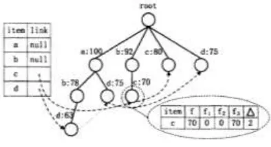
called a prefix-tree. A complete tree is as shown in Figure 1.

As shown in Figure 1, the sliding window in the tree contains three base windows. The node c marked in the chart represents that the number of data item set

 

b,c in the sliding window is 70, the estimated error is defined to be 2, and the order of magnitude

 

b,c is 0, 0, 70 in the following windows.

Figure 1. Example of a tree.

According to the characteristics of the data win-dows for mining frequent items, a data stream can be divided into blocks Ni(i1,2,...). The length of each

block is Ni 

 

1/



or an integral multiple of

 

1/



. For easier description, here we take

 

1/



i

N and each data block still contains  1/

identifiers. This way, we can call the window of the data block a base window that is _w_i₍_i₁_,₂_,...). In the sliding window, W can contain k continuous base windows, where k has to be preset. The presetting and initial settings of critical frequent items are given in Table 1 below.

Table 1. The initial settings of critical frequent items.

Item f f1 f2 f3



a 100 0 0 100 2

b 92 0 0 92 2

c 80 0 0 80 2

d 75 0 0 75 2

The number of base windows contained in the slid-ing window W is regarded as k.

Output: Update the tree

(1)Store the wnew data into the tree;

(2)If (f-list is empty) is generated into an f-list; (3)Else for each item ei



f-list //sliding window, the unqualified information is deleted;

(4)

{

e

i

.

f



e

i

.

f



e

i

.

f

1

;

if

(





0

)

(5) for(j1;jk;j){ei,fjei.fj1;}ei.fk0} //corresponds to row (4);

(6)for each item ei



wnew //corresponds to each

item set in the new window;

(7)

{

if

(

e

_i



f



list

)

e

_i

.

f

_k



e

_i

f

_k_₁

;

//if it belongs to the f-list, the number of counts is added by 1;

(8)else //insert new information; (9)

{

insert

ei into f-list; ei.fk=1; △=k-1;

(10)for(j1;jk;j){e_i.f_j 0;}} //corresponds to row (9);

(11) for each item ei



f-list

(12)

{

.

;

k i i i

f

e

f

e

f

e





(13)if(ei.fk) delete ei; } //corresponds to

row (12);

(14)Arrange the f-list in a descending order accord-ing to the f value of each row.

2.3 Result analysis of frequent item mining

When each new transmitted data enters the sliding window, a new tree will be built. During this process, the initial information window will be updated and replaced, and the information of non-frequent items will be gradually deleted from the process chart of the tree.

[image:4.516.264.463.371.448.2]

First, the initial data have to be standardized. That is, the two best items above and the four dimensions in the BSC system are compared in pairs to obtain a comparison table of the reference layer as shown in Table 2 below:

Table 2. Comparison result of reference layer.

A B C D Row Geometric Mean

Feature Vector

A 1 3 5 6 0.581 2.364

B 1/3 1 2 3 0.203 0.828

C 1/5 1/2 1 2 0.140 0.586

D 1/6 1/3 1/2 1 0.076 0.321

Then the arithmetic mean of each row is calculated: 080

. 3 6 5 3 1

4

1    

w

075 . 1 3 2 1 3 / 1

4

2    

w

740 . 0 2 1 2 / 1 5 / 1

4

3     

w

408

.

0

1

2

/

1

3

/

1

6

/

1

4







w

The data are then normalized:

303 . 5

4 3 2 1 4

1

    





w w w w w

i

303 . 5

080 . 3

4

1 1

1 





(5)

In the same way, we have: 203

. 0

2

w , w₃0.140, w40.076 The feature vector is calculated:

   

 

   

 

    

 

   

 

    

 

   

 

321 . 0

586 . 0

828 . 0

346 . 2

076 . 0

140 . 0

203 . 0

581 . 0

1 3 / 1 2 / 1 6 / 1

2 1 2 / 1 5 / 1

3 2 1 3 / 1

6 5 3 1

111 . 4 076 . 0

321 . 0 140 . 0

586 . 0 203 . 0

828 . 0 581 . 0

346 . 2 4 1 ) ( 1

1

max 

  



 _ _ _

 





n

i i

i

w Aw n



[image:5.516.263.462.77.158.2]

According to the judgment matrix and feature vec-tors of the target layer of the mined items, we have the results shown in Tables 3, 4, 5 and 6.

Table 3. Index judgment matrix and feature vectors for finance.

A1 A2 A3 A4 A5 Row Geometric Mean

Feature Vector

A1 1 4 5 2 3 2.605 0.416 A2 1/4 1 3 1/3 1/2 0.660 0.105 A3 1/5 1/3 1 1/4 1/3 0.353 0.056 A4 1/2 3 4 1 2 1.643 0.262 A5 1/3 2 3 1/2 1 1.000 0.161

According to calculation: max5.200

Table 4. Index judgment matrix and feature vectors for users.

B1 B2 B3 B4 Row Geometric Mean

Feature Vector

B1 1 2 1/3 1/4 0.639 0.136 B2 1/2 1 1/2 1/3 0.537 0.114 B3 3 2 1 1/2 1.316 0.280 B4 4 3 2 1 2.213 0.470

Table 5. Index judgment matrix and feature vectors for internal businesses.

C1 C2 C3 C4 C5 Row Geometric Mean

Feature Vector

C1 1 1/2 1/4 1/3 1/2 0.461 0.073 C2 2 1 1/2 4 3 1.643 0.263 C3 4 2 1 5 4 2.759 0.441 C4 3 1/4 1/5 1 1 0.786 0.126 C5 2 1/3 1/4 1 1 0.608 0.097

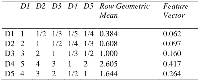
Table 6. Index judgment matrix and feature vectors for learning and innovation.

D1 D2 D3 D4 D5 Row Geometric Mean

Feature Vector

D1 1 1/2 1/3 1/5 1/4 0.384 0.062 D2 2 1 1/2 1/4 1/3 0.608 0.097 D3 3 2 1 1/3 1/2 1.000 0.160 D4 5 4 3 1 2 2.605 0.417 D5 4 3 2 1/2 1 1.644 0.264

3 CONCLUSIONS

One of the most popular algorithms of finding Fre-quent Items in data streams using Extensible and Scalable Bloom Filter based on Landmark window model (FI-ESBFL), which deeply explores the essen-tials of data stream frequent item mining algorithm over decaying window and frequent item judgment based on sliding window model. Theoretically, books and academic papers on finance-related risk evalua-tion, including commercial researches on bank credit risks, are pouring into our eyes at an unprecedented speed.

Some researchers have made intensive discussions from credit risk management and other perspectives. Research methods for the application of bank credit risks are becoming enriched and matured. This paper further determines the threshold of credit risks with historic sample sets and maintenance sample sets, using the summary information in credit risks, achieves relatively accurate threshold precision with certain storage spaces and provide theoretical guid-ance for risk management.

REFERENCES

[1] Wang Yan. 2004. Discussion on association rule in data mining. Journal of Chengdu University of Information Technology, 02: 172-176.

[2] Dai Xiaoting. 2014. Analysis of Association Rule Min-ing Algorithm and Its Application in Intelligent Logis-tics. Science Technology and Industry, 02: 113-116. [3] People’s Bank of China Guangzhou Branch Project

Team, Zhen Runzan, Liang Wei. Research on the Finan-cial Credit Data Application in Regional Credit Risk Monitoring. South China Finance, 2014, 04: 31-36+19. [4] Ding Liping, & Lu Guoqing. 2014. Survey of Differen-tial Privacy in Frequent Pattern Mining. Journal on Communications, 10: 200-209.

[image:5.516.53.251.251.349.2]

(6)

[6] Qu Wu, Sui Haifeng, Yang Bingru, & Xie Yonghong. 2012. Advances in Study of Distributed Mining of Data Streams. Computer Science, 01: 1-8+36.

[7] Xiao Tiaogen. 2012. Research on Credit Risk Index and Early Warning. Credit Reference, 02: 86-89.

[8] Ma Chaoqun, Ding Yu, & Zhang Hong. 2006. Research on Commercial Bank Credit Risks and Their Measure-ment Model. Modern Management Science, 10: 5-6. [9] Li Shujie. 2006. Applied Research about Commercial

Bank Risk Measurement Model. Finance Teaching and Research, 05: 19-22.

[10] Yu Ruifeng, Ren Yanmin, Wang Yu, & Liu Liwen. 2007. Research on Risk Assessment of Corporate Credit Based on Supply Chain. Chinese Journal of Manage-ment Science, 03: 85-92.