Numerical Simulation of Vortex Street Around the Two Dimensional Cylinder Based on LES

2020 4th International Conference on Modelling, Simulation and Applied Mathematics (MSAM 2020) ISBN: 978-1-60595-674-9

Numerical Simulation of Vortex Street Around the Two-Dimensional

Cylinder Based on LES

Hai-run SONG

, Shu-dao ZHOU

, Xiao-lei WANG

,

Song YE

and Zhen-tao CHEN

1

College of Meteorology and Oceanography, National University of Defense Technology, Nanjing 211101, China

2

Collaborative Innovation Center on Forecast and Evaluation of Meteorological Disasters, Nanjing University of Information Science & Technology, Nanjing 210044, China

*Corresponding author

Keywords: Karman vortex street, Vortex, Boundary layer, Flow around circular, Large Eddy Simulation (LES).

Abstract. In order to study the characteristics of the Karman vortex street generated in the flow around the bluff body, this paper uses the numerical model of the large eddy simulation to numerically simulate the flow around the two-dimensional cylinder. Combined with the simulation data, this paper validates and analyzes the Karman vortex phenomenon, and studies the properties of the vortex shedding when the boundary layer is separated in the flow around the cylinder. The simulation results show that the inflow around the cylinder will produce two different characteristics of the vortex. The high velocity vortex is generated outside the boundary layer, and the small velocity vortex is generated inside the boundary layer, and the two alternately fall off to form the vortex street; When the size of the flow-through cylinder is constant, the falling vortex increases with the increase of the flow velocity, and when the flow velocity increases to a certain value, the vortex size will remain unchanged; When kept constant, the vortex is positively correlated with the size of the cylinder. The results obtained in the paper describe the Carmen vortex street generated in the flow around the two-dimensional cylinder in a relatively detailed way. Finally, this paper provides a reference for studying turbulent energy dissipation and boundary layer separation.

Introduction

The phenomenon of flow around a cylinder exists widely in nature and engineering. Although the structure of the cylinder is simple, its surrounding flow will involve multiple complex problems such as boundary layer separation, vortex shedding, and turbulent interaction [1]. Therefore, the flow around a cylinder has always been an important subject in the study of fluid mechanics. Under certain conditions, Carmen vortex street phenomenon will occur when the cylinder flows around. And, it is important in this phenomenon that as the Reynolds number increases, the nature of the turbulence and the vortex shape will change greatly [2]. Therefore, the study of the Carmen vortex street in the flow around a cylinder is of great significance for solving complex problems such as turbulent dissipation and boundary layer separation.

At present, the flow around a cylinder is mainly divided into two aspects: two-dimensional flow and three-dimensional flow. T.K.Prasanth [3] compared the flow around a double cylinder with that of a single cylinder. K.P. Wang and X.C. Zhao [4] carried out a numerical simulation of the lateral excited vibration of a two-dimensional cylinder. Karniadakis et al. [5] analyzed the Reynolds number in Three-dimensional numerical simulation of the flow around a cylinder between 100 and 500 was performed. Lei [6] analyzed the influence of the size of the calculation domain on the accuracy of three-dimensional flow around a cylinder.

formation. Secondly, we used Fluent to numerically simulate different incoming flow velocities and different cylinder diameters. Finally, we analyzed the simulation results in conjunction with the Carmen vortex street phenomenon, and studied the effects of different incoming flow velocities and different cylinder diameters on the vortex size. This article provides a reference for studying turbulent energy dissipation and fluid barrier boundary layer separation.

Formation of Vortex and Carmen Vortex Street

When the viscous fluid adheres to the surface of the fluid-blocking fluid, a frictional force is generated, which hinders the movement of the fluid in the thin layer near the solid wall. In this thin layer, the velocity of the fluid close to the solid wall is zero, and gradually returns to the fluid velocity outside the frictionless force as it moves away from the solid wall. This thin layer, called the boundary layer, is the area formed from the surface of the object to the fluid that is not subject to friction [7].

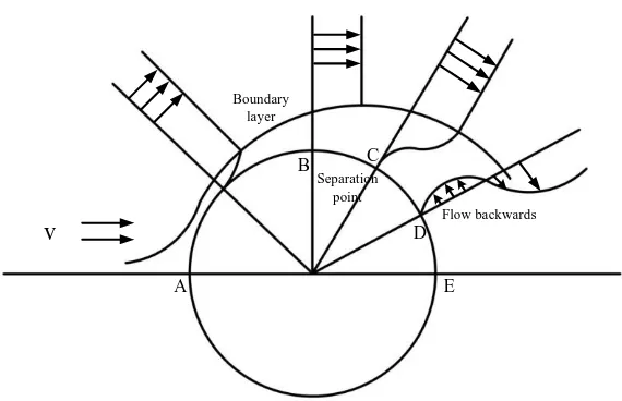
If the fluid encounters a bluff body, then the fluid will pass through the bluff body and it will separate the boundary layer. In fluid flow, the separation of the boundary layer is closely related to the pressure distribution of the boundary layer. We take the flow around a cylinder as an example, as shown in Figure 1. When the incoming flow reaches the foremost point A on the surface of the bluff body’s surface, its speed will decrease to zero and the pressure will increase to a maximum value. In a non-viscous flow, the fluid particles are accelerated on the upstream surface from point A to point B, and decelerated on the downstream surface from point B to point E. Therefore, the particle pressure of the fluid from point A to B decreases, and the particle pressure of the fluid from B to E increases. Outside the boundary layer, pressure from point A to point B is transformed into kinetic energy, and from point B to point E is transformed into pressure. Therefore, the speed at which fluid particles reach point A and point E should be equal. However, in general, the motion of the flow field is viscous. In viscous flow, a thin boundary layer will be formed on the surface of the bluff body at the moment when the flow starts. In the boundary layer, the fluid is subjected to high frictional forces. In the process from point A to point B, the fluid particle will consume a large amount of kinetic energy, so that the remaining kinetic energy is too small to overcome the "pressure barrier" from point B to E, making it from point B to E The boost area at point will not go too far and will stop at point C. Then, the pressure of the external fluid will force the subsequent fluid including the point D to flow in opposite directions, thereby forming a reverse flow. The fluid outside the boundary layer still flows forward, and the fluid inside the boundary layer flows backward, thereby forming a vortex motion, and the vortex no longer moves against the solid wall and falls off.

v B C A D Boundary layer Flow backwards Separation point E

Figure 1. Schematic diagram of boundary layer separation.

Mathematical Model and Numerical Simulation Method

Control Equation of Numerical Simulation

The turbulence numerical simulation methods provided by CFD include three methods: direct numerical simulation method, Reynolds average method and large eddy simulation method. When large eddy simulation is used, it will deal with large-scale and small-scale eddies in the flow field. Large-scale vortices are directly solved using filtered Navier-Stokes equations, and small-scale vortices are solved using a subgrid tension scale model. Large eddy simulation is based on turbulence statistical theory and the understanding of pseudo-sequence structure. In this way, large eddy simulation not only saves computer resources, but also captures more complete flow field flow information [9]. Therefore, this paper mainly uses the large eddy simulation on the high Reynolds number to study the flow around the two-dimensional cylindrical plane.

After effective filtering of the filter function, the Navier-Stokes equation for large-scale eddies can be obtained [10]:

0 i i u t x      

  (1)

( ) ( ) i ij

i i j

j j j i j

u p

u u u

t x x x x x



    

   

  _ _ 

   _  _   (2)

In equations (1) and (2),  is the fluid density,  is the fluid viscosity, ui _and uj _{are the filtered}

velocity components, p is the filtered pressure, and ij _{is the sub-grid tension. The sub-grid tension} can be defined as:

ij u ui j u ui j

   (3)

Aerodynamic Parameters of Turbulence

Re UL 

 (4)

In formula (4), U is the incoming flow velocity of the flow field, and L is the characteristic length of the object.

Dynamic Viscosity Of Fluid. The dynamic viscosity of the fluid is closely related to the local temperature. When the temperature T <2000 K, the dynamic viscosity of the fluid can be calculated using the Sutherland formula [12]:

1.5 0

0 0

T C

T

T T C

 

    

    _ 

 

  (5)

In formula (5), 0 _{is the dynamic viscosity value at T = T0 = 288.15 K, and C is Sutherland}

constant.

Density Of Fluid. When the gas is in a thermodynamic equilibrium state, its pressure, density and temperature will meet certain relationships. The commonly used equation of state for a complete gas is:

pRT (6) Where R is the general gas constant. The density of the gas is

p RT

 (7)

Mathematical Model

The mathematical model used in the simulation is a two-dimensional cylinder flow model, the diameter of the two-dimensional cylinder is D = 0.2 cm, the rectangular calculation area of the simulation is 60 D × 10 D, in which the distance between the cylinder plane and the flow inlet is 2 D, the distance from the flow outlet is 57 D, and the distance from the upper and lower boundaries of the calculation area is 4 D. The fluid moves from left to right, and the leftmost side is the inlet of calculation domain, which adopts the boundary condition of velocity inlet; the rightmost side is the outlet of calculation domain, which adopts the boundary condition of pressure outlet; the upper and lower boundaries and two-dimensional cylinder plane adopt the wall condition without sliding. In order to improve the accuracy of the calculation, the unstructured triangular mesh is used and the two-dimensional cylinder plane boundary is encrypted. There are 19994 element meshes in total, as shown in Figure 2.

Figure 2. Mathematical model and its mesh generation.

Table 1. Calculation parameter.

Area Reynolds number Diameter of the cylinder D/m

Velocity of flow field /m/s

Numerical simulation method

Low Reynolds number

66.4 0.02 0.1

Laminar flow

132.8 0.02 0.2

256.6 0.02 0.4

331.9 0.02 0.5

High Reynolds number

398.3 0.02 0.6

LES

531.1 0.02 0.8

663.9 0.02 1

1327.8 0.02 2

2655.6 0.02 4

Simulation Results and Analysis

Carmen Vortex Phenomenon

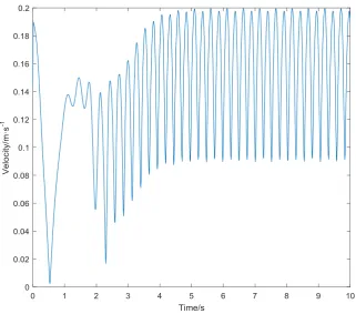
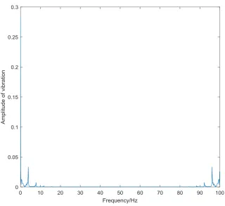
We have studied the formation of Carmen vortex street around a cylinder with a flow velocity of 2 m/s. The simulation results consist of a time series with a time step of 0.01 s and a length of 10 s. We select the point with coordinates (10, 10) in the two-dimensional plane to observe the change in the velocity of the flow field during the formation of the vortex street, as shown in Figure 3. It can be seen from the figure that in the time period of t = (0 ~ 4) s, the velocity of this point shows a non-periodic change, which indicates that the vortex is being formed during this period, and the vortex street has not been reached Conditions; and within the time after t = 4 s, the velocity of the flow field clearly shows periodic changes, indicating that a mature vortex street has been formed. As shown in Figure 4, we can get the spectrum information by Fourier transform of the discrete-time velocity sequence of this point. From the spectrum information diagram, we can get the corresponding frequency according to the peak position, that is, the frequency of vortex street change, which is 3.9 Hz.

Figure 4. The velocity spectrum analysis graph with coordinates (10, 10).

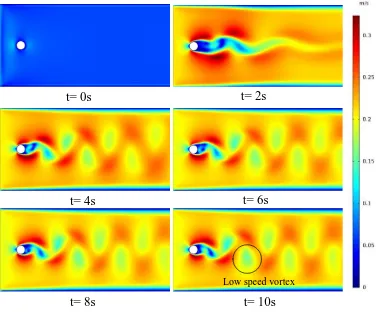
Figure 5 selects the contour maps of the velocity at six representative moments when the velocity of the flow field is 2 m/s. The figure shows the formation and dissipation of a vortex street. At t = 0 s, the velocity of the flow field has not yet played a role, and vortices have not yet formed. At t = 2 s, a vortex is being formed, and two vortices with different velocity distributions are formed, one with a high speed is outside the boundary layer, and one with a low speed is inside the boundary layer. At t = 4 s, the left and right sides of the two-dimensional cylinder alternately form mature vortices, and a vortex street is formed after the two-dimensional cylinder. At t = 6 s, the initially formed vortex is moving forward and has reached the entrance boundary. At t = 8 s, the vortex with a small velocity starts to dissipate after a certain distance.

t= 0s t= 2s

t= 4s t= 6s

t= 8s t= 10s

The Effect of the Velocity of the Flow Field on the Vortex

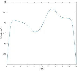
The formation of the vortex is mainly related to the dissipation of energy in the boundary layer when the fluid bypasses the bluff body. In order to study the energy change during fluid motion, it is necessary to study the properties of small velocity vortices in the boundary layer. Figure 6 shows the cloud near the cylinder when the velocity of the flow field is 2 m/s It can be seen from the figure that the velocity of the small velocity vortex formed in the boundary layer gradually increases from the center to the outside, and its outer diameter is always surrounded by the velocity value at the edge of the boundary layer from formation to elimination. Therefore, the vortex can be regarded as a circle with a continuously changing diameter, and the velocity value at the edge of the boundary layer can be used as a threshold for obtaining the outer diameter of the vortex. We take the first mature vortex formed at t = 10 s in Figure 4 as an example, and select the velocity value of the cross section of x = 18.5 cm.

t= 0s t= 2s

t= 4s t= 6s

t= 8s t= 10s

Low speed vortex

Figure 7. Speed curve of x = 18.5 cross section at 10s when the flow field velocity is 2 m/s.

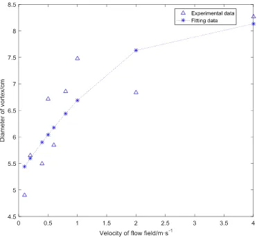
Figure 8. Curve of vortex diameter as a function of flow field velocity at t = 10 s.

The Effect of the Size of the Bluff Body on the Vortex

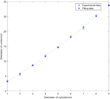
Figure. 9. Curve of vortex diameter as a function of cylinder diameter at t = 10 s when the flow field velocity is 2 m/s.

Conclusions

The paper is based on the CFD simulation method and uses numerical simulation methods of large eddy to perform numerical simulations on cylinders with different inflow speeds and diameters. Among them, this paper studies the formation of Carmen vortex street, analyzes and discusses the influence of incoming flow velocity and cylinder size on vortices, and draws the following conclusions:

The computational fluid dynamics software can successfully simulate the Carmen vortex street phenomenon, and can clearly reflect the generation and dissipation of vortices. In the process of generating the vortex around a two-dimensional cylinder, the velocity of the flow field and the diameter of the cylinder will affect the size of the vortex diameter. When the diameter of the cylinder is constant, the shedding vortex will increase with the increase of the flow field velocity. However, when the flow velocity increases to a certain value, the size of the vortex diameter will remain unchanged. When the velocity of the flow field is kept constant, the size of the vortex diameter is positively related to the diameter of the cylinder.

References

[1] L. Wang, T.Y. Li, X. Zhu, W.J. Guo, Improved immersed boundary lattice Boltzmann method and simulation of flow over rotating cylinder, Chin. J. Ship. Res. 11 (2016) 97-103.

[2] D. Sumner, Flow above the free end of a surface-mounted finite-heigth circular cylinder: a reiew, J. Fluid. Struct. 43 (2013) 41-63.

[3] T.K. Prasanth, S. Mittal, Flow-induced oscillation of two circular cylinders in tandem arrangement at low Reynolds number, J. Fluid. Struct. 25 (2009) 1029-1048.

[4] K.P. Wang, X.Z. Zhao, Research about lift and drag coefficient of circular cylinder oscillating transverse to the flow, J. Jiangsu. U. Sci. Tech. 31 (2017) 579-585.

[5] G.E. Karniadakis, G.S. Triantafyllou, Three-dimensional dynamics and transition to turbulence in the wake of bluff objects, J. Fluid. Mech. 238 (1992) 1-30.

[6] C. Lei, L. Cheng, K. Kavanagh, Spanwise length effects on three-dimensional modelling of flow over a circular cylinder, Comput. Method. APPL. M. 190 (2001) 2909-2923.

[7] J.Y. Liu, Extension of field synergy principle for convective heat transfer to high speed compressible boundary-layer flows, Chin. J. Aeronaut. 39 (2018) 131-140.

[8] H. Wang, B. Jin, G. Yao, Research and Design of Broadband Underwater Flow Induced Vibration Energy Harvester Based on Karman Vertex, Chin. J. Sen. Actuat. 32 (2019) 469-475.

[9] Y. Zhou, M.M. Alam, Wake of two interacting circular cylinders: a review, Int. J. Heat. Fluid. Fl. 62 (2016) 510-515.

[10] Z.S. Zhang, Turbulen, National Defense Industry Press, Beijing, 2002.

[11] L. Chen, J.Y. Tu, G.H. Yeoh, Numerical simulation of turbulent wake flows behind two side-by-side cylinders, J.Fluid.Struct. 18(2003) 387-491.