[NORMAL] GPU cluster for acceleration of scientific and engineering applications in the context of higher education

(1)

University of Huddersfield Repository

Newall, Matthew

GPU cluster for acceleration of scientific and engineering applications in the context of higher

education

Original Citation

Newall, Matthew (2015) GPU cluster for acceleration of scientific and engineering applications in

the context of higher education. Masters thesis, University of Huddersfield.

This version is available at http://eprints.hud.ac.uk/id/eprint/23746/

The University Repository is a digital collection of the research output of the

University, available on Open Access. Copyright and Moral Rights for the items

on this site are retained by the individual author and/or other copyright owners.

Users may access full items free of charge; copies of full text items generally

can be reproduced, displayed or performed and given to third parties in any

format or medium for personal research or study, educational or notforprofit

purposes without prior permission or charge, provided:

•

The authors, title and full bibliographic details is credited in any copy;

•

A hyperlink and/or URL is included for the original metadata page; and

•

The content is not changed in any way.

For more information, including our policy and submission procedure, please

contact the Repository Team at: [email protected].

(2)

UNIVERSITY

OF

HUDDERSFIELD

GPU Cluster for Acceleration of Scientific

and Engineering Applications in the

Context of Higher Education

Author:

Matthew NEWALL

Supervisor: Dr Violeta HOLMES

A thesis submitted in fulfilment of the requirements for the degree of Masters By Research

High Performance Computing School Of Computing and Engineering

(3)

1

Copyright Statement

• The author of this thesis (including any appendices and/or schedules to this the-sis) owns any copyright in it (the Copyright) and s/he has given The University of Huddersfield the right to use such Copyright for any administrative, promotional, educational and/or teaching purposes.

• Copies of this thesis, either in full or in extracts, may be made only in accordance with the regulations of the University Library. Details of these regulations may be obtained from the Librarian. This page must form part of any such copies made.

(4)

2

Abstract

Many fields of research now rely on High Performance Computing (HPC) systems which can process ever larger datasets, with increasing accuracy and speed. Many universities now provide a HPC service. Following the trend over the past few years of the worlds fastest supercomputers being accelerated using Graphical Processing Units (GPUs), there is a growing interest in the use of GPUs in Higher Education Institutions. The characteristics of GPUs make them excellently suited to any task exhibiting a high level of data parallelism. Recent developments in GPU technologies have focused on improving performance and integration in HPC, and for processing data other than dis-play graphics.

To investigate the benefits such a system could have to the University of Huddersfield, a small GPU cluster has been deployed. The intention behind this thesis is to detail the deployment of the system and to demonstrate, through case studies, the required effort a potential user could expect in order to take advantage of it.

(5)

3

Acknowledgements

(6)

4

Contents

Copyright Statement 1

Abstract 2

Acknowledgements 3

List of Figures 6

List of Tables 7

Abbreviations 8

1 Introduction and Background 9

1.1 Aims and Objectives . . . 10

1.2 Methodology . . . 10

2 Literature Review 12 2.1 GPUs as general purpose processors . . . 12

2.1.1 GPU Programming Frameworks . . . 15

2.1.1.1 Nvidia CUDA . . . 15

2.1.1.2 openCL . . . 16

2.2 Obstacles to using GPUs for scientific calculations . . . 17

2.3 Scientific applications of current GPU technology . . . 18

2.4 HPC Systems which use GPUs . . . 19

2.4.1 TITAN - Oak Ridge National Laboratory . . . 20

2.4.2 Emerald . . . 20

3 Vega GPU Cluster 22 3.1 The Microsoft Windows HPC Platform . . . 22

3.2 Cluster Layout . . . 23

3.3 Deployment . . . 24

3.4 Testing . . . 25

4 Platforms and Programming Environments for Scientific Data Visualisation and Processing 31 4.1 Visualisation . . . 32

(7)

Contents 5

4.3 GPU Programming Framework . . . 33

5 Case Study 1: Visualisation of large datasets 35 5.1 Electron Microscopy Data . . . 35

5.2 VisIt . . . 36

5.3 Evaluation of Results . . . 37

6 Case Study 2: Accelerated Processing of Radio Telescope Data Using CUDA 39 6.1 The SETIFFT software . . . 40

6.1.1 Optimising CUDA performance . . . 41

6.1.2 Using MPI to increase performance . . . 42

7 Case Study 3: CUDA Accelerated Analysis of Wavelength scanning Inter-ferometry Data 46 7.1 The Interferometry Software . . . 46

7.2 Improving Performance Using MPI . . . 47

8 Conclusion 50

9 Further Work 52

A SILOWRITE tool 53

B SETIFFT sonification code 58

C Wavelength Scanning Interferometry Software 74

D GPU Cluster for Accelerated processing and Visualisation of Scientific

Data 90

E Delivering faster results through parallelisation and GPU acceleration 97

(8)

6

List of Figures

2.1 Architecture of the Nvidia GeForce 6800 GPU, showing pipelined design with separate units for Vertex processing, Rasterization and Blending

(Nvidia, 2006) . . . 14

2.2 Architecture of the Nvidia TESLA GPU, showing unified design with gen-eral purpose streaming processors (Lindholm et al., 2008) . . . 14

2.3 A representation of the graphics pipeline as implemented on CUDA GPUs (Luebke and Humphreys, 2007) . . . 15

3.1 Current VEGA hardware layout and network topology. . . 24

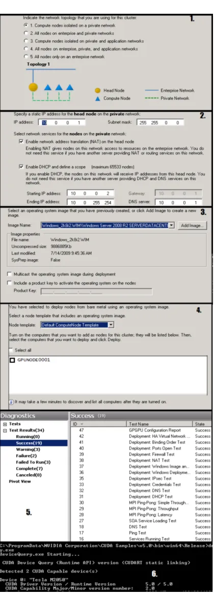
3.2 Key steps when deploying VEGA: 1. Selecting Network Topology 2. Con-figuring NAT and DHCP to allow compute nodes to access outside net-work 3. Creating a system image for compute nodes 4. Finding bare metal machines to deploy as compute nodes 5. Checking relevant diag-nostic tests pass 6. Checking CUDA functionality . . . 26

3.3 Tuning HPL parameters using Lizard . . . 27

3.4 Simple MPI test program, based loosely on the example from Matto-torang (2009) . . . 28

3.5 Output from MPI test program when run on all cores . . . 29

3.6 GPU test programs included with CUDA toolkit (Nvidia, 2013a), from top to bottom: Device Query, Testing Aligned Types, Matrix Multiplication . . 30

5.1 Visualisation method before VisIt . . . 36

5.2 Program flow for the SILOWRITE code . . . 37

5.3 Comparison of Visualisation methods, from top to bottom: Original spread-sheet, 2D Mesh in VisIt, 3D mesh in VisIt, 3D contour mesh in VisIt . . . . 38

6.1 Program flow of the SETIFFT software . . . 40

6.2 Program flow of the initial MPI program . . . 43

6.3 Program flow of the final MPI version . . . 44

6.4 Total running times of each version . . . 45

7.1 Program flow for the original CUDA code . . . 47

7.2 Program flow for the MPI version using multiple GPUs . . . 48

7.3 Total running times for each version . . . 49

(9)

7

List of Tables

3.1 Hardware available for VEGA . . . 23

6.1 Timings for original JAVA program . . . 40

6.2 Timings for Java program with wrapped CUDA functions . . . 41

6.3 Timings for C++ with serial FFT . . . 41

6.4 Timings for C++ with CUFFT . . . 41

6.5 Timings for C++ with CUFFT and MPI, running on multiple GPUs . . . 42

6.6 Timings for C++ with CUFFT and MPI, running on multiple GPUs . . . 42

(10)

8

Abbreviations

GPU GraphicsProcessingUnit

HPC HighPerformanceComputing

AD ActiveDirectory

QGG QueensGateGrid

CUDA ComputeUnifiedDeviceArchitecture

MPI MessagePassingInterface

API ApplicationProgrammingInterface

(11)

9

Chapter 1

Introduction and Background

High Performance computing systems are now well established as an essential tool for research and analysis in Higher Education. A High Performance computing system is one which uses multiple computers to carry out one task, through parallel processing. Many Universities have some kind of HPC provision. At the University of Huddersfield a number of HPC systems have been deployed for the use of researchers and students (Kureshi, 2010). These systems are used regularly for tasks such as large CFD simula-tions, running MPI software, image rendering and more. However, the fastest computer HPC systems now include Graphic Processing Units (GPU) (Top500, 2013a). This research is attempting to answer the following questions

• Why do we need an alternative to CPU systems for scientific processing

• Why are GPUs so suited to this task

• What issues would be faced in deploying a GPU system.

• How would such a system support research in a Higher Education institution such as the University of Huddersfield.

(12)

Introduction and Background 10

1.1

Aims and Objectives

The overall goal of this project was to investigate the viability of a GPU cluster to compli-ment the HPC provision available at the University of Huddersfield. The key objectives for success were:

• Investigate the application of GPU technologies in HPC systems.

• Evaluate existing GPU systems in the context of Higher Education to support scientific research.

• Deploy a GPU cluster within a HE institutional grid.

• Investigate different platforms and programming environments for the purpose of highly parallel task and data processing and visualisation.

• Evaluate the suitability of the GPU cluster using representative case studies.

• Propose possible future developments of the system to accelerate HE scientific research.

The final outcome of this project was considered to be a functional GPU cluster, suc-cessfully integrated as part of the HPC provision at the university, justified through a number of case studies.

1.2

Methodology

In order investigate how best to achieve the project aims and objectives, a compre-hensive literature review was conducted, A GPU cluster was deployed and integrated into the campus grid, and case studies were carried out to evaluate its usefulness in supporting the visualisation and processing of data.

The result of this study is presented in this thesis and is organised as outlined below:

(13)

Introduction and Background 11

• Chapter 3: Design and deployment of a GPU cluster is described.

• Chapter 4: Outlines a selection of appropriate software, platforms, and program-ming environments for visualisation and processing of data, based on the litera-ture.

• Chapter 5,6, and 7: Presents the results of testing the usefulness and suitability of the cluster through three representative case studies.

(14)

12

Chapter 2

Literature Review

2.1

GPUs as general purpose processors

There have been numerous efforts up to this point to use GPUs as general purpose processors. An important concept to bear in mind when establishing the suitability of an algorithm or program for processing on a GPU is arithmetic intensity, which as stated by Harris (2005), is the ratio of computation to bandwidth. This is significant as computational speed currently increases more rapidly than communication speed, so memory access latency will negate potential computational speedup. Problems with a high arithmetic intensity are those which exhibit a high level of data parallelism, and have minimal dependency between data points.

(15)

Literature Review 13

on the GPU through its hardware projection matrix, which has been programmed to perform the Hough Transform (Fung and Mann, 2005, chap. 3.2).

Efforts have also been made to abstract the process of GPU acceleration to high level operations. Tarditi et al. (2006) describe Accelerator; ”a system that uses data paral-lelism to program GPUs”. Accelerator allows programmers to accelerate suitable parts of their code using GPU accelerated functions, without exposing any aspect of the GPU. Unlike the traditional approach, which would involve compiling the data-parallel parts of the program as shader programs in native code, Acellerator compiles GPU parts of the code on the fly at runtime. Using this software Tarditi et al. (2006) were able to demon-strate an acceleration of up to 18 times over native C code running on a CPU. While it does not match the performance of hand written GPU code, its simplicity of use makes it an important step towards accessible GPU acceleration.

As the use of GPUs as accelerators became increasingly common, GPU manufacturers started to change the design of their units accordingly. Fig. 2.1 Shows the architecture of the Nvidia GeForce GPU; it is a design highly specialised to graphics with hardware designed to fulfil specific parts of the graphics pipeline, as was the case most GPUs up to this point. As can be seen in Fung and Mann (2005, chap. 3.2), and Tarditi et al. (2006, chap. 3.1), programming GPUs required determining which part of the graphics pipeline was best suited to the problem, and could require vastly different approaches depending on which part of the GPU was targeted. To use the full pipeline often meant numerous copies to and from host memory as it was not possible to utilise the internal transports on the GPU.

(16)

FIGURE2.1: Architecture of the Nvidia GeForce 6800 GPU, showing pipelined design with separate units for Vertex processing, Rasterization and Blending (Nvidia, 2006)

(17)

FIGURE 2.3: A representation of the graphics pipeline as implemented on CUDA GPUs (Luebke and Humphreys, 2007)

2.1.1 GPU Programming Frameworks

2.1.1.1 Nvidia CUDA

As well as the CUDA platform itself, Nvidia actively develop a programming model for its GeForce, Quadro and Tesla processors. It is highly scalable and will run on an ar-bitrary number of processors without the need to recompile. This is required because of the vast and varying number of processor cores in modern GPUs (Nvidia, 2008). As observed by Garland et al. (2008), the CUDA framework allows a programmer to use the massively multi-threaded nature of GPUs for a wide range of highly parallel problems. While this was possible previously, using graphics APIs, CUDA relieves the programmer of the requirement of intimate knowledge of the target hardware. Addition-ally, it removes the daunting task of having to negotiate a complicated and unfamiliar language, as was previously the case when targeting different parts of the graphics pipeline. All of this allows the programmer to instead ”focus on the important issues of parallelism - how to craft efficient parallel algorithms” (Garland et al., 2008, chap. 2).

CUDA programs consist of two parts;

(18)

• Parallel kernels - CUDA kernels are scalar sequential programs which execute on the GPU. These sequential programs operate on a grid of thread blocks, and must be able to be execute independently.

As an example, consider the loop in Listing. 1.1 The code iterates over a grid of data and performs the function at each point one at a time. The parallel version in listing. 1.2 performs the same function, but rather than looping through, each point is processed essentially simultaneously. (Garland et al., 2008)

v o i d serial_function (i n t n, f l o a t a, f l o a t _*x, f l o a t _*y) {

f o r (i n t i = 0 ; i<n; i++)

y[i] = a_*x[i] + y[i] ; }

/ / p e r f o r m on 1M elements

serial_function_{(4 096 *256 , 2.0 ,} x, y) ;

LISTING2.1: A standard C function

v o i d gpu_function (i n t n, f l o a t a, f l o a t _*x, f l o a t _*y) {

i n t i = blockIdx.x_*blockDim.x + threadIdx.x;

i f (i<n) y[i] = a_*x[i] + y[i] ; }

/ / p e r f o r m on 1M elements

gpu_function<<4096, 256>>(n, 2 . 0 , x, y) ;

LISTING 2.2: The same function as might be written for execution on a CUDA

supported GPUNvidia (2013a)

2.1.1.2 openCL

(19)

f l o a t gpu_function (f l o a t a, f l o a t _*x, f l o a t _*y) {

r e t u r n y = a_*x + y; }

kernel v o i d function(global write_only y, global a, global x) {

i n t i=get_global_id( 0 ) ;

y[i] =gpu_function( 2 . 0 , x[i] , y[i] ) ; }

LISTING2.3: An example of a functiuon as might be written for OpenCL

2.2

Obstacles to using GPUs for scientific calculations

There are a number of caveats which must be kept in mind when using GPUs for cal-culations for which they were not designed. Graphics processing is highly tolerant to small errors so GPUs have not traditionally included error checking and correcting (ECC) memory systems. Scientific calculations, on the other hand, are highly sensitive to error. In response to this uncertainty, Haque and Pande (2010) have investigated the implications of using GPUs with non-ECC memory in non graphics calculations.By running a memory test program on more than 50,000 GPUs from the Folding@Home project, it was demonstrated that there is a statistically significant probability of transient errors occurring in GPU memory.

However, in response to the requirements of the scientific research community, GPU manufacturers have developed architectures specifically designed for general purpose processing.

(20)

Even with ECC RAM there may be other precautions required when considering floating point accuracy on GPUs. While Nvidia GPUs with compute capability 2.0 and higher (Tesla M series and onwards) are compliant with the same IEEE 754 standard as CPUs for double precision floating point operations, Whitehead and Fit-florea (2011) suggest that there may be further precautions required to ensure accuracy when using Nvidia GPUs. There are fundamental differences in rounding modes on GPUs when compared to x86. as described in Whitehead and Fit-florea (2011, chap. 4.7) ”rounding modes are encoded within each floating poin instruction instead of dynamically using a floating point control word”. Unlike CPUs, There is no mechanism to indicate overflowed or underflowed calculations, or calculations with inexact logic. This implications of this are discussed later in the paper; while it is possible to produce the best floating point result for simple math operations, problems arise with more complex functions. While the same input will yeild the same results in an individual IEEE 754 compliant operation, differences in the potential sequencing of operations in GPUs, compared to CPUs, may mean differences in numerical results, even in newer hardware.

The authors offer some recommendations to ensure accuracy and performance; taking advantage of CUDA library functions (which have been written with these caveats in mind), careful comparison of results, and knowledge of the capabilities of the specific GPU being used.

2.3

Scientific applications of current GPU technology

GPUs have found use in a wide variety of fields. Cardenas-Montes et al. (2014) De-scribe their efforts at performing an accurate calculation of cosmic shear using GPUs. Cosmic shear describes the distortion of the observed shapes of distant galaxies as their light passes through gravitational potential, a phenomenon known as gravitational lensing. According to Cardenas-Montes et al. (2014), measuring cosmic shear allows the mass distribution causing the distortion to be derived. This ultimately allows the measurement of the accelerated expansion of the universe.

This calculation is highly computationally intensive, fitting with O(N2₎_{, and it is}

(21)

The code is written for an Nvidia Tesla c1070 card, which is a Fermi architecture card. When compared to the same calculation performed on the CPU, the new GPU code represents a 68-fold speed increase. While this shows that GPUs are very powerful if you have the right problem, it also highlights the importance of well considered memory management when constructing GPU programs. The authors demonstrated that the best performance could only be achieved after tuning copy patterns, chunk size, and cache utilization.

Anthopoulos et al. (2013) offer an improved GPU acellerated cell-list approach. Cell-lists are important in the field of molecular dynamics as they are used to show atomic interactions within a given radius. Again, not only is this problem highly computationally expensive, but it is not trivial to parallelise.

The authors benchmarked their improved algorithm extensively both for speed, an ac-curacy compared to the same algorthm when run on a CPU. Total runtime is measured as well as each discrete part of the process, this allows more detailed anaysis of where the best performace gains are, and which areas perhaps require further optimisation. To test accuracy it was deemed an unfair test to directly compare CPU and GPU re-sults due to the differences in rounding methods on both as mentioned earlier. Instead, double precision results from the CPU code were cast to single then back to double precision to remove the need to presume rounding error in non-GPU code. Accuracy in this case is measured as deviation from the CPU results, and is shown to be accurate to four significant figures.

2.4

HPC Systems which use GPUs

(22)

2.4.1 TITAN - Oak Ridge National Laboratory

Titan has a peak performance of 17.59 PetaFlops, and was once Number one in the Top500 supercomputer sites (Top500, 2013b), as of November 2013 it is still number 2. It has 18,658 nodes, standard ones ”each with a 16 core AMD opteron 6274 proces-sor and an Nvidia tesla K20 GPU” (ORNL, 2011b) as well as over 700 Terra-bytes of memory. Titan demonstrates well the space and power efficiency of GPUs, as despite occupying the same space as its predecessor, Jaguar, and only using marginally more power, Titan outperforms Jaguar by a factor of 10 (1.75 PFlops for Jaguar as compared to 17.59 for Titan) owing to the fact that it has a much higher ratio of GPUs to CPUs.

Researchers working with ORNL (2011a) put extensive consideration, in the years be-fore Titan was completed, into appropriate software which would be able to take full advantage of Titans then unique configuration. A selection of 6 codes was made, all from different scientific disciplines. These codes were then adapted to allow them to use the system to its full capability. These efforts highlight the importance of an aware-ness of the capabilities of specific hardware within a GPU cluster. Poor planning and lack of consideration of memory capacity and throughput, particularly in a GPU, can have a drastic effect on the performance of software.

Some of the problems Titan is used to solve include: Nanoscale materials analysis, to aid development of new magnets to improve designs of motors and generators; de-tailed modelling of the combustion of fossil fuels with the aim of improving the efficiency of internal combustion engines, and to reduce their impact on the environment; and detailed atmospheric modelling, to further climate change research.

2.4.2 Emerald

(23)

(24)

22

Chapter 3

Vega GPU Cluster

Investigation into existing GPU systems currently being used to accelerate scientific computation has demonstrated a significant speedup of simulations, modelling and vi-sualisation. In order to evaluate the benefit such a system could have for research at the university of Huddersfield it was necessary to deploy a small GPU cluster. This chapter details the assembly, installation and testing of this system. The cluster is in-tegrated into the University campus network and is accessible internally by students and staff. The Microsoft Windows HPC server software was used to deploy the GPU cluster.

3.1

The Microsoft Windows HPC Platform

Microsoft provides tools to allow deploying and managing a cluster using Microsoft Windows Server. Microsoft (2014c) detail the deployment of a complete HPC system using Microsoft tools.

(25)

VEGA GPU Cluster 23

MPI-2 standard (Microsoft, 2014a). It is compatible with MPICH2, which makes porting MPI code from other platforms, such as Linux, relatively simple.

3.2

Cluster Layout

The following hardware was available for the deployment:

Item Description

Netgear ProSafe GSM7224 24 port Gigabit network switch

Dell Poweredge R410 1x Quad core octo-thread Xeon E 5630 CPU running at 2.53 GHz, 32 GB RAM. Dell Poweredge C6100 4 node chassis currently with 2 nodes

installed. each with the following spec: 2x Quad core octo-thread Xeon E5620 CPUs, running at 2.4GHz, 24 GB RAM, and approx 400GB local storage.

Dell Poweredge C410x PCIe Ex-pansion Chassis + 1 interface card

This chassis can host up to 16 GPUs and is connected to a compute node using a PCIe interface card (Dell, 2014)

2x Nvidia Tesla M1020 GPUs These are FERMI architecture cards with 448 processor cores running at 1.15 GHz, with 3GB of ECC GDDR5 RAM with a clock speed of 1.546 (Nvidia, 2013e)

TABLE3.1: Hardware available for VEGA

As the Poweredge C6100 is a four node chassis, it was selected to act as compute node. There is only a single PCIe interface card available so initially there is only a single compute node, with the option of adding more in the future. The Poweredge R410 acts as head node.

(26)

VEGA GPU Cluster 24

FIGURE3.1: Current VEGA hardware layout and network topology.

3.3

Deployment

Initially, all hardware was tested to ensure it was viable. According to the deployment procedure outlined by Microsoft (2014c), was to install Windows Server 2008r2, which is a standard procedure. Once installed, the Head node is connected to the university network and then added to Active Directory by specifying the domain name. At this point the following steps are performed to deploy the GPU cluster:

(27)

VEGA GPU Cluster 25

• The head node is attached to the private Gigabit switch.

• Compute nodes are deployed by first connecting them to the Private network then booting to PXE. The Windows HPC software will then load an operating system and required middleware over the network. This differs from the procedure offered by Microsoft (2014c), which suggests attaching nodes which have already been configured with windows server and HPC pack. As the nodes did not already have Windows installed, it was deemed much simpler to have the head node push out preconfigured system images to the compute node.

• Finally, drivers for the TESLA cards are installed on the compute node directly (Nvidia, 2013c).

A summary of the deployment steps required to deploy the GPU cluster, VEGA, can be seen in Fig. 3.2.

3.4

Testing

The Windows HPC cluster manager includes a number of diagnostic tests to verify clus-ter deployment. All relevant tests when run on VEGA passed without any problems. The standard measure of performance of HPC systems, and the test used to measure sys-tems for inclusion in the top500, is the LINPACK benchmark. The benchmark consists of ”a dense system of linear equations”(Jack Dongarra and Stewart, 2013), and the ability of a system to process these is used as a measure of peak performance. The parallel implementation of LINPACK is known as High Performance LINPACK (HPL). Microsoft provides a self-tuning HPL utility, Lizard, to benchmark Windows clusters, the results and final tuned parameters of this can be seen in Fig. 3.3. This however does not include the extra performance provided by the GPUs, figures from Nvidia state that peak theoretical performance of each M2050 is 1.03 TFLOPS (Nvidia, 2013e).

(28)

VEGA GPU Cluster 26

FIGURE3.2: Key steps when deploying VEGA: 1. Selecting Network Topology

2. Configuring NAT and DHCP to allow compute nodes to access outside network 3. Creating a system image for compute nodes

4. Finding bare metal machines to deploy as compute nodes 5. Checking relevant diagnostic tests pass

6. Checking CUDA functionality

Windows was chosen as the operating system to allow familiarity with users, and easy integration with the existing active directory network. In addition, running Windows allows the option of adding the cluster to the backburner render system in use at the university.

However, CUDA is also available for Linux. Were it required, necessary drivers are available to allow the same functionality, using a cluster middleware such as OSCAR or Warewulf (ORNL, 2005), (LBL, 2014).

(29)

VEGA GPU Cluster 27

Parameter N NB PMAP P Q Threshold

Final Value 44992 304 0 2 12 16

Parameter PFACT NBMIN NDIV RFACT BCast Depth

Final Value 0 4 8 2 1 1

Parameter SWAP L1 U Equilibration Alignment

Final Value 2 0 0 0 16

CPU only performance = 95.02 GIGAFLOPS

(30)

VEGA GPU Cluster 28

# i n c l u d e ” s t d a f x . h ”

# i n c l u d e <i o s t r e a m>

# i n c l u d e ” mpi . h ”

# i n c l u d e<Winsock2 . h>

#pragma comment ( l i b , ” Ws2 32 . l i b ”)

using namespace std;

i n t main(i n t argc, char_* argv[ ] ) {

i n t nTasks, rank;

MPI_Init(&argc,&argv) ;

MPI_Comm_size(MPI_COMM_WORLD,&nTasks) ;

MPI_Comm_rank(MPI_COMM_WORLD,&rank) ;

char hname[ 1 2 8 ] = ” ”;

WSADATA wsaData;

WSAStartup(MAKEWORD( 2 , 2 ) , &wsaData) ;

gethostname(hname, s i z e o f(hname) ) ;

WSACleanup( ) ;

printf (” Number o f t h r e a d s = %d , My rank = %d\n , My Host = %s ”, nTasks, rank, hname)←

-;

MPI_Finalize( ) ;

r e t u r n 0 ; }

(31)

VEGA GPU Cluster 29

Number of threads = 24 , My rank = 10 , My Host = GPUNODE0001

Number of threads = 24 , My rank = 16 , My Host = VEGA

(32)

VEGA GPU Cluster 30

(33)

31

Chapter 4

Platforms and Programming

Environments for Scientific Data

Visualisation and Processing

There is a need to develop parallel programming environments to aid software develop-ment for parallel computer architectures. However, other than those already outlined in chapter 2, there are still few mature parallel programming environments. Perhaps more important is the absence of tools and IDEs that allow for simple debugging and testing of parallel software with the ease and reliability of those established for traditional serial programs. This is particularly true for software designed to make use of accelerators. While debugging and development tools do exist for accelerators such as GPUs, they are platform specific (for example Nvidia Nsight (Nvidia, 2014)) meaning that develop-ing parallel software for heterogeneous systems remains a comparatively convoluted process.

(34)

Platforms and Programming Environments for Scientific Data Visualisation and

Processing 32

4.1

Visualisation

Visualisation of scientific data is not a novel concept. Matlab is used extensively to plot 2D and 3D images. Similarly, CFD and MD packages such as ANSYS (INC, 2014) and DL POLY (STFC, 2014) provide inbuilt software for visualisation of processed data. When evaluating the available visualisation software for deployment on VEGA, VisIt, a parallel visualisation tool, was chosen for its focus on parallel processing using MPI, as well as GPU accelerated rendering. In addition, it boasts compatibility with a vast range of CAD, CFD, MD, graphing and mathematics software (LLNL, 2013). VisIt is highly flaxible in the data it can display, thanks to software functions which allow data to be structured appropriately programatically, in C or FORTRAN.

4.2

Multi-Node parallelism

An integral part of any HPC system is a mechanism to allow programs to utilise multi-ple CPU cores which do not necessarily occupy the same host node. MPI has proven itself over the past couple of decades in this regard and has become a standard used in the vast majority of HPC deployments. MPI supports a wide selection of program-ming languages such as C++ and and Java (Forum’, 2014). Some key concepts to consider when using MPI; Communicators, Point to Point operations, and Broadcast and Collection. Communicators are used to group MPI processes related to the same task. Most MPI operations must specify a communicator, this ensures that the oper-ation only effects those processes which are in the same communicator (for example MPI COMM WORLD). Point to Point operations, such as MPI Send and MPI Recv, are used to send data from one rank to another in a one to one relationship. Broadcast and Collection operations such as MPI Bcast and MPI Scatter are one to many or many to one operations, and are useful for dividing data among processes, and then collecting after processing.

(35)

Processing 33

integrated with the Windows HPC job scheduler, the scheduler used in VEGA, allowing simple submission of MPI tasks to the cluster. This close integration makes MSMPI par-ticularly suited for Multi-node parallel software when Windows HPC is used (Microsoft, 2014b).

Options other than MPI include OpenMP which allows ”multi platform shared memory parallel programming” (Board, 2013). This offers some flexibility when developing par-allel software. The programming experience is very similar to that of using MPI, with the added benefit of shared memory. Parallel Virtual Machine (PVM) is an approach which aggregates discrete systems which do not necessarily need to have the same hardware or operating system. PVM allows a heterogenous cluster of machines to appear as a single virtual machine (ORNL, 2009).

4.3

GPU Programming Framework

(36)

Processing 34

so programs which use multiple GPUs must take care to check which GPU is being requested to avoid crashing.

(37)

35

Chapter 5

Case Study 1: Visualisation of

large datasets

As models and datasets become larger and more complex, new systems are required to enable useful analysis. To support the need of researchers at the University, it was deemed necessary to deploy a visualisation tool which could work with large or complex datasets.

To this end, and existing software, VisIt, was obtained and installed on VEGA. VisIt is a software developed by the Lawrence Livermore National Laboratory (LLNL), described as ”Parralel, Interactive, Visualisation” (LLNL, 2013). It is specifically designed to utilise HPC resources to enable interactive simulation of terrascale datasets, and supports GPU accelerated rendering.

5.1

Electron Microscopy Data

(38)

Case Studies 36

energy of a point on a cylinder, and the values change over time. The spreadsheet that was in use was unwieldy and cannot all be seen at once as seen in Fig 5.1. This made proper analysis difficult, ideally the data would be shown as points on an actual cylinder as a 3D contour. For these reasons the data was deemed a good candidate for case study.

FIGURE5.1: Visualisation method before VisIt

5.2

VisIt

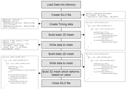
Visit displays data that is defined on 2D or 3D meshes, this presents a challenge; The electron microscopy data is simply a comma delimited list of values. The solution was to build a software tool to format this data, and save it to an appropriate file format. The SILO library was developed by LLNL fo use with VisIt in situations such as this, and allows production of data meshes programmatically (LLNL, 2010). Following the recommendations in the SILO users guide, the software was built uses standard SILO functions to save the data in 3 different formats:

• A 2D mesh where the data is represented by colour (similar to the function of the original spreadsheet)

(39)

Case Studies 37

• and finally a 3D mesh which deforms based on the value of each point over time (contour).

Fig. 5.2 shows a summary of important parts of the program, full listings can be seen in appendix 1.

FIGURE5.2: Program flow for the SILOWRITE code

5.3

Evaluation of Results

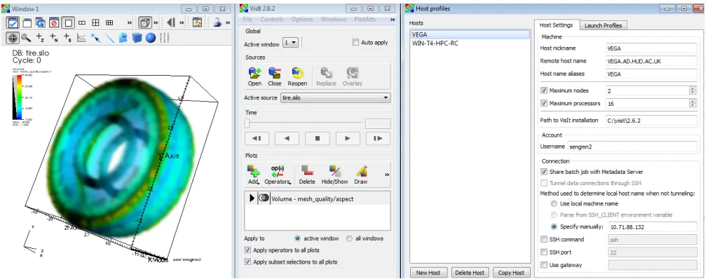
Fig. 5.3 Shows a few images of each visualisation method at different time steps. The final 3D contour model fulfils the original requirements of the project and allows real time interactive analysis of the simulation data. The main advantage of this model is that all the data for each time step can be seen at once. The animation can be easily saved to video.

[image:39.596.112.519.186.474.2]

(40)

Case Studies 38

FIGURE 5.3: Comparison of Visualisation methods, from top to bottom: Original spreadsheet, 2D Mesh in VisIt, 3D mesh in VisIt, 3D contour mesh in VisIt

(41)

39

Chapter 6

Case Study 2: Accelerated

Processing of Radio Telescope

Data Using CUDA

(42)

Case Studies 40

6.1

The SETIFFT software

In order to sonify the data, a piece of software was written in JAVA by Paul Lunn for the Sonic SETI project. Fig. 6.1 shows the program logic. In order to asses which parts of the software would best benefit from acceleration, different sections of the code were timed, these timings can be seen in Table 6.1. In each test, the software performs 244 FFTs using a 2GB file as input, measurements are averaged over 10 separate runs.

FIGURE6.1: Program flow of the SETIFFT software

Action Time Taken (Ms)

Read data 3713182 (1:01:53)

Perform FFT 4491666 (1:13:52)

Calculate Power Spectrum 477218 (0:07:57)

Save to File 1344062 (0:22:24)

Total run time 10026326 (2:47:06)

TABLE6.1: Timings for original JAVA program

(43)

Case Studies 41

Read data 3801657 (01:03:22)

Perform FFT 916464 (00:15:16)

Save to File 1404548 (0:23:25)

Total Run Time 5711437 (1:35:11)

TABLE6.2: Timings for Java program with wrapped CUDA functions

In order to improve read and write time, and to make better use of CUDA functions, the program was rewitten in C++, first with a serial FFT as seen in table 6.3, then with CUFFT as seen in table 6.4.

Read data 29686 (0:00:27)

Perform FFT 1541246 (0:25:41)

Save to File 29686 (0:00:30)

Total Run Time 1810008 (0:30:10)

TABLE6.3: Timings for C++ with serial FFT

Read data 17344

Perform FFT 90720

Calculate Power Spectrum 70781

Save to File 17344

Total run time 277674

TABLE6.4: Timings for C++ with CUFFT

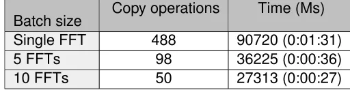
6.1.1 Optimising CUDA performance

(44)

Case Studies 42

Batch size Copy operations Time (Ms) Single FFT 488 90720 (0:01:31)

5 FFTs 98 36225 (0:00:36)

10 FFTs 50 27313 (0:00:27)

TABLE6.5: Timings for C++ with CUFFT and MPI, running on multiple GPUs

Making these changes decreased FFT processing time for a 2GB file by 63.4 seconds, an improvement of over 69%.

6.1.2 Using MPI to increase performance

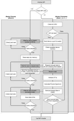
To utilise the second GPU in the system, and to allow the program to scale to even larger systems, the program was modified to implement MPI. Fig. 6.2 shows the pro-gram structure of the initial version. Files are read and written by the master process rank, and data is sent to and from the worker ranks using MPI.

This initial MPI version was successful in reducing actual processing time, but the large MPI data transfers added significant overhead, in excess of any performance gained in processing. The solution was to make use of the shared storage available on VEGA to remove the need for large MPI send/recieve operations. Fig. 6.3 shows the structure of the final version of the software. Rather than data being sent to each rank using MPI functions, each rank opens the relevant file directly. In this version MPI messages are only used to tell the workers which files to open and where to start and stop reading.

Table. 6.6 shows timings for the final code. Each rank processes a share of the data, and are timed simultaneously , hence two timings for each section of the program.

Action Time Taken (Ms)(rank 0) Time Taken (rank 1)

Read data 118043 145642

Perform FFT 12310 12570

Calculate Power Spectrum 40271 40304

Save to File 118043 145642

Total run time 249777

[image:44.596.185.441.82.148.2] [image:44.596.119.509.583.680.2]

(45)

Case Studies 43

FIGURE6.2: Program flow of the initial MPI program

6.2

Evaluation of Results

It can be seen that read/write time is increased in the MPI version compared to the sin-gle process. This is because each process is accessing the same file simultaneously. Table 6.7 shows times when the program is run with two files from the dataset. As the datasets are often larger than 8GB, they are split into 2GB files (SETI, 2013a), so this would not be outside the normal use of the software.

[image:45.596.201.461.86.511.2]

(46)

Case Studies 44

FIGURE6.3: Program flow of the final MPI version

(47)

Case Studies 45

Files Total FFTs Read/Write time

1 244 145642

2 488 145816

TABLE6.7: Read/write time for the MPI software when reading from different numbers of files

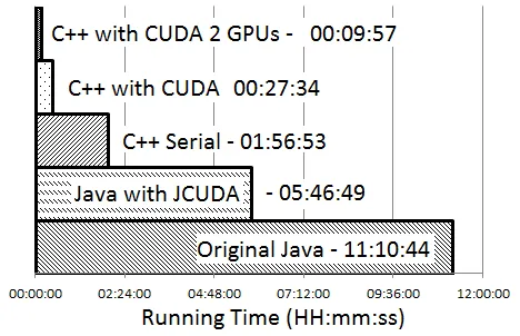
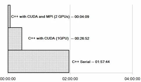
Figure 6.4 compares total running times of each significant version of the software, run-ning with a full dataset 5GB in size (split into 2GB files). Through parrallelisation (using both CUDA and MPI) and optimisation it has been possible to significantly accelerate the process of sonifying the radio telescope data.

FIGURE6.4: Total running times of each version

[image:47.596.164.470.82.134.2] [image:47.596.199.433.272.423.2]

(48)

46

Chapter 7

Case Study 3: CUDA Accelerated

Analysis of Wavelength scanning

Interferometry Data

Optical interferometry is a widely used surface metrology technique. Wavelength scan-ning interferometry developments have been made that allow the process to be immune to environmental noise using phase compensation. However this compensation as well as data analysis processes limit performance, and hamper efforts to inspect this data as the measurement takes place. The paper Muhamedsalih et al. (2012) details a method which uses CUDA to accelerate this process with a single GPU. However, while the results were promising, it wass still not possible to achieve the real time analysis that was desired.

7.1

The Interferometry Software

(49)

Case Studies 47

FIGURE7.1: Program flow for the original CUDA code

7.2

Improving Performance Using MPI

(50)

Case Studies 48

FIGURE7.2: Program flow for the MPI version using multiple GPUs

7.3

Evaluation of Results

(51)

Case Studies 49

FIGURE7.3: Total running times for each version

(52)

50

Chapter 8

Conclusion

Existing GPU clusters were evaluated, with a focus on the Higher Education context and scientific research. This research allowed informed decisions regarding the deployment of our own system, and lead to the deployment of VEGA, a small GPU cluster integrated into to campus network forming part of the institutional grid. With this system in place it was possible to investigate and evaluate different platforms and programming envi-ronments to support the goal of highly parallel task and data processing. Using case studies the suitability of the GPU cluster was evaluated. The first case study showed that useful visualisation of seemingly abstract data could be achieved using the appro-priate platforms, and enabled a level of analysis previously not possible for this data. By using the CUDA GPU programming model, as well as MPI, significant performance gains were possible, both for sonification of radio telescope data, and analysis of wave-length scanning interferometry data. While the initial objective was to use CUDA with Java and C++ to accelerate applications using multi-core GPU devices, It has been possible to achieve even greater performance gains though implementation of multi-system MPI code, to allow multiple GPUs to process data. Not only will the CUDA implimentations scale automatically to larger, faster GPUs, but MPI allows scaling to multi node GPU clusters.

(53)

Conclusion 51

(54)

52

Chapter 9

Further Work

The case studies detailed here have been designed to scale to much larger systems through using MPI. Running the software on larger systems will allow the efficiency and performance of the software to be assessed, giving opportunity to discover bottlenecks and develop more concrete methods for software design on GPU clusters.

(55)

53

Appendix A

SILOWRITE tool

# i n c l u d e <s i l o . h>

# i n c l u d e <f s t r e a m>

# i n c l u d e <sstream>

# i n c l u d e <s t r i n g>

# i n c l u d e <v e c t o r>

u s i n g namespace std;

c o n s t f l o a t pi = 3.14159265359;

i n t main(i n t argc, char _*argv[ ] ) {

i n t NX= 360;

i n t NY= 100;

i n t NZ= 1 ;

i n t nnodes = NX_*NY_*NZ;

i f(argc<3) {

cerr<< ”USAGE: ”<<argv[0]<<” 100 / / ( t i m e i n ns ) 10.0 / / r a d i u s ”<<endl;

system(” pause ”) ;

r e t u r n ₋1; }

stringstream tim, radi, mul;

tim<<argv[ 1 ] ;

radi<<argv[ 2 ] ;

(56)

Appendix A.SILOWRITE tool 54

i n t maxtime;

tim>>maxtime;

f l o a t radius,multiplier;

radi>>radius;

mul>>multiplier;

f l o a t _* x=new f l o a t[nnodes] ;

f l o a t _* y=new f l o a t[nnodes] ;

f l o a t _* z=new f l o a t[nnodes] ;

f l o a t _*data=new f l o a t[nnodes] ;

f o r (i n t time= 0 ; time<=maxtime; time++) {

/ * Open i n p u t data * /

ostringstream oss;

oss << ” data / ” << time << ” ns . d a t ”;

string fname = oss.str( ) ;

string _*str;

str=new string[nnodes] ;

f l o a t _*indata;

indata=new f l o a t[nnodes] ;

ifstream file(fname) ;

i n t i = 0 ;

i f( !file) / / Always t e s t t h e f i l e open . {

cout<<

” E r r o r opening i n p u t f i l e ,

e i t h e r i n c o r r e c t path s p e c i f i e d

o r i n s u f f i c i e n t data ”<<endl;

system(” pause ”) ;

r e t u r n −1; }

w h i l e( !file.eof( ) ) {

getline(file,str[i] ,' ') ;

i f(i ==nnodes−1) {

i= 0 ;

getline(file,str[i] ,' ') ; }

i++; }

f o r (i n t i= 0 ; i<nnodes;i++) {

(57)

DBfile _*dbfile = NULL; / * Open the S i l o f i l e * /

char filename[ 1 0 0 ] ;

sprintf (filename, ” o u t p u t / o u t%04d . s i l o ”, time) ;

dbfile = DBCreate(filename, DB_CLOBBER, DB_LOCAL, ” s i m u l a t i o n t i m e s t e p ”, DB_HDF5) ;

i f(dbfile == NULL) {

fprintf(stderr, ” Could n o t c r e a t e S i l o f i l e !\n ”) ;

r e t u r n −1; }

/ * Copy i n data * /

f o r (i n t i= 0 ; i<nnodes;i++) data[i] =indata[i] ; / * Add t i m i n g data f o r V i s I t * /

DBoptlist _*optlist = DBMakeOptlist( 2 ) ;

DBAddOption(optlist, DBOPT_CYCLE, (v o i d _{* ) &}time) ;

DBAddOption(optlist, DBOPT_DTIME, (v o i d _{* ) &}time) ; / * Create Geometry * /

f l o a t rad= 0 ; / * 3D Mesh * /

f o r(i n t iY= 0 ;iY<NY;iY++) {

f o r (i n t iX= 0 ;iX<NX;iX++) {

f o r (i n t iZ= 0 ;iZ<NZ;iZ++) {

rad=iX_{* (}pi/ 1 7 9 ) ;

x[iY_*NZ_*NX+iX_*NZ+iZ] =radius_*cos(rad) ;

y[iY_*NZ_*NX+iX_*NZ+iZ] =iY−50;

z[iY_*NZ_*NX+iX_*NZ+iZ] =radius_*sin(rad) ; }

(58)

i n t dims[ ] = {NX, NY, NZ};

i n t ndims = 3 ;

f l o a t _*coords[ ] = {(f l o a t_{* )}x, (f l o a t_{* )}y, (f l o a t_{* )}z};

DBPutQuadmesh(dbfile, ” C y l i n d e r ”, NULL, coords, dims, ndims,

DB_FLOAT, DB_NONCOLLINEAR, optlist) ; / * Add data * /

dims[ 0 ] = NX; dims[ 1 ] = NY; dims[ 2 ] = NZ;

DBPutQuadvar1(dbfile, ” 3D”, ” C y l i n d e r ”, data, dims,

ndims, NULL, 0 , DB_FLOAT, DB_NODECENT, NULL) ; / * 2D Mesh * /

f o r (i n t iZ= 0 ;iZ<NZ;iZ++) {

x[iY_*NZ_*NX+iX_*NZ+iZ] =iX;

y[iY_*NZ_*NX+iX_*NZ+iZ] =iY−50; }

} }

i n t dims2[ ] = {NX, NY};

ndims = 2 ;

f l o a t _*coords2[ ] = {(f l o a t_{* )}x, (f l o a t_{* )}y};

DBPutQuadmesh(dbfile, ” FlatMesh ”, NULL, coords2, dims2, ndims,

dims[ 0 ] = NX; dims[ 1 ] = NY; ;

DBPutQuadvar1(dbfile, ” F l a t ”, ” FlatMesh ”, data, dims,

ndims, NULL, 0 , DB_FLOAT, DB_NODECENT, optlist) ; / * 3D countour mesh * /

f l o a t radiuscont;

i= 0 ;

(59)

{

rad=iX_{* (}pi/ 1 7 9 ) ;

radiuscont=radius+data[i_{] *}multiplier;

i++;

x[iY_*NZ_*NX+iX_*NZ+iZ] =radius_*cos(rad) ;

y[iY_*NZ_*NX+iX_*NZ+iZ] =iY−50;

z[iY_*NZ_*NX+iX_*NZ+iZ] =radius_*sin(rad) ; }

} }

i n t dims3[ ] = {NX, NY, NZ};

ndims = 3 ;

f l o a t _*coords3[ ] = _{(f l o a t_{* )}x, (f l o a t_{* )}y, (f l o a t_{* )}z};

DBPutQuadmesh(dbfile, ” Contour ”, NULL, coords3, dims3, ndims,

dims[ 0 ] = NX; dims[ 1 ] = NY; dims[ 2 ] = NZ;

DBPutQuadvar1(dbfile, ” 3DContour ”, ” Contour ”, data, dims,

ndims, NULL, 0 , DB_FLOAT, DB_NODECENT, optlist) ; / * Close the S i l o f i l e . * /

DBFreeOptlist(optlist) ;

DBClose(dbfile) ; }

d e l e t e[ ] x,y,z,data;

r e t u r n 0 ; }

(60)

58

Appendix B

SETIFFT sonification code

Original program written by Paul Lunn for the SonicSETI project (SETI, 2013b). It was modified extensively and mostly rewritten to take advantage of multiple GPUs. Memo-ryMapped is a function written by Brumme (2014) and is used here to handle the large input files.

# i n c l u d e <s t d i o . h>

# i n c l u d e <s t r i n g . h>

# i n c l u d e <math . h>

# i n c l u d e <t i m e . h>

# i n c l u d e <mpi . h>

# i n c l u d e <v e c t o r>

# i n c l u d e <sys / s t a t . h>

# i n c l u d e ” cuComplex . h ”

# i n c l u d e <Winsock2 . h>

#pragma comment ( l i b , ” Ws2 32 . l i b ”)

# i n c l u d e <c u d a r u n t i m e . h>

# i n c l u d e <c u f f t . h>

# i n c l u d e <cuda . h>

# i n c l u d e <h e l p e r f u n c t i o n s . h>

# i n c l u d e <h e l p e r c u d a . h>

# i n c l u d e ” s e t i f i l e . h ”

/ / MPI TAGS

(61)

Appendix B.SETIFFT sonification code 59

# d e f i n e RANGE 2

# d e f i n e MEM 3

# d e f i n e DATA 4

# d e f i n e PI 3.14159265358979323846

i n t myrank, totalranks;

MPI_Status Stat;

/ /−=−=−=−=−=−=−=−=−=−=−=−=−=−=−=−=−=−=−=−=−=−=−=−=−=−=−=−=−

i n t checkErrors(i n t err) {

i f (err>1) r e t u r n 1 ;

s w i t c h(err) {

case 1 : r e t u r n 1 ;

d e f a u l t: std: :cout<<” Something ' s wrong ! ? ! ? ”<<std: :endl;break;

case 0 : std: :cout<<”_\n_\nRequired :_\n '₋i f <path>' s p e c i f i e s t h e path t o t h e _←

-i n p u t f i l e ( s ) . There can be any number o f these , a t l e a s t one i s r e q u i r e d\n\←

-nOptions :\n−v Enables p r o g r e s s messages , may i n c r e a s e r u n t i m e\n−d Enables debug ←

-mode , w i l l d e f i n i t e l y i n c r e a s e r u n t i m e\n−t P r i n t s t i m i n g i n f o r m a t i o n\n−h e l p ←

-Shows the se h i n t s ”<<std: :endl; break;

case −1: std: :cout<<” Could n o t open i n p u t f i l e ! ”<<std: :endl;break;

case −2: std: :cout<<” Could n o t open o u t p u t f i l e ! ”<<std: :endl;break;

case ₋3: std: :cout<<” Problem w r i t i n g t o o u t p u t f i l e ! ”<<std: :endl;break;

case −4: std: :cout<<” Problem a l l o c a t i n g GPU! ”<<std: :endl;break;

case −5: std: :cout<<” Problem r e a d i n g from i n p u t f i l e ! ”<<std: :endl;break; }

Sleep( 2 0 0 0 ) ;

i f (err <= 0 ) exit( 1 ) ;

r e t u r n 0 ; }

i n t concatinateFiles(c o n s t std: :vector<std: :string> &fileNames)/ / t h i s b i t i s 100% n o t←

-p o r t a b l e and i s a l m o s t c e r t a i n l y -poor form , b u t i t s f a s t e r than r e a d i n g i n t h e _←

-f i l e s ( Were a l r e a d y u s i n g windows . h anyway )

{ / / j o i n s m u l t i p l e f i l e s _{w i t h f i l e n a m e f o r m a t *}<i n t e g e r>.<e x t e n s i o n>

size_t numFiles = fileNames.size( ) ;

std: :string command;

std: :stringstream ss;

ss<<” copy ”;

(62)

{

ss<<fileNames[i]<<” ”; }

ss>>command;

system(command.c_str( ) ) ;

r e t u r n 1 ; }

b o o l checkExistance (c o n s t std: :string& name) {

s t r u c t stat b;

r e t u r n (stat(name.c_str( ) , &b) == 0 ) ; }

i n t cleanUp(c o n s t std: :vector<std: :string>&fileNames) {

size_t numFiles = fileNames.size( ) ;

std: :vector<std: :string> concFiles;

std: :string concChk;

i n t file= 0 ;

f o r (i n t i= 0 ;i<=0;i=i) {

concChk=fileNames[file] +std: :to_string(i) ;

i f(checkExistance(concChk) ) {

concFiles[i] =concChk;

i++; }

e l s e

{

concatinateFiles(concFiles) ;

file++; }

}

r e t u r n 1 ; }

i n t main(i n t argc, char _{* *}argv) {

i n t totalranks, myrank, master = 0 ;

MPI_Status Stat;

MPI_Request sreq = MPI_REQUEST_NULL;

MPI_Request_* rreq;

i n t exit= 0 ;

/ / OPTIONS ( s e t i n command s w i t c h e s )−=−=−=−=−=−=−=−=−=−=−=−

i n t verbose=f a l s e;

(63)

/ /−=−=−=−=−=−=−=−=−=−=−=−=−=−=−=−=−=−=−=−=−=−=−=−=−=−=−=−=−

MPI_Init(&argc,&argv) ;

MPI_Comm_size(MPI_COMM_WORLD, &totalranks) ;

MPI_Comm_rank(MPI_COMM_WORLD, &myrank) ;

rreq = new MPI_Request[totalranks] ;

i n t fftPower=23;

std: :vector<std: :string> fileNames;

i n t fileCount= 0 ;

/ / parse o p t i o n s / use d e f a u l t s

i f(myrank==master) std: :cout << argv[0]<<” ”;

i f (argc < 1&&myrank==master) {

r e t u r n checkErrors( 0 ) ; }

MPI_Barrier(MPI_COMM_WORLD) ;

f o r (i n t i = 1 ; i < argc; i++) {

i f(myrank==master) std: :cout << argv[i]<<” ”;

i f (std: :string(argv[i] ) == ”₋i f ”) {

(fileNames.push_back(argv[++i] ) ) ;

fileCount++; }

e l s e i f (std: :string(argv[i] ) == ”−v ”) {

verbose=atoi(argv[++i] ) ; }

e l s e i f (std: :string(argv[i] ) == ”−d ”) {

debug=t r u e; }

e l s e i f (std: :string(argv[i] ) == ”−h e l p ”&&myrank==master) {

e l s e i f (myrank==master) {

}

(64)

i f(debug&&myrank==master) {

std: :cout << ” I n p u t once debugger i s a t t a t c h e d . . . ” << std: :endl;

std: :cin.get( ) ; }

MPI_Barrier(MPI_COMM_WORLD) ; / /−=−=−=−=−=−=−=−=−=−=−=−=−=−=−

i n t range[ 3 ] = {0 , 0 , 0}; / / f i r s t f i l e , f i r s t f f t , t o t a l f f t s

b o o l data=t r u e;

char instruction = 0 ;

i n t totalFFTs= 0 ;

i n t fftsPerNode= 0 ;

i f (myrank == master) {

b o o l_* skiprank=new b o o l[totalranks] ;

b o o l_* GPUrank=new b o o l[totalranks] ;

f o r(i n t i= 0 ;i<totalranks;i++) {

skiprank[i] =f a l s e;

GPUrank[i] =f a l s e; }

i n t gpus= 0 ;

rreq[i] = MPI_REQUEST_NULL;

char testgpu=f a l s e;

MPI_Recv(&testgpu, 1 ,MPI_CHAR,i,MSG,MPI_COMM_WORLD,&Stat) ;

i f(testgpu) gpus++;

e l s e skiprank[i] =t r u e;/ / ra nk s w i t h o u t gpus are s k i p p e d }

/ / D i v i d e data based on number o f gpus

i n t _*totalFFTsInFile = new i n t [fileCount] ;

(65)

checkErrors(totalFFTsInFile[i] =SETIFILE: :getNumFFTs(fileNames[i] ,fftPower←

-) -) ;

totalFFTs+=totalFFTsInFile[i] ; }

fftsPerNode=totalFFTs/gpus;

i n t rem=totalFFTs%gpus;

i n t file= 0 ;

i n t sentTotal= 0 ;

i n t sentTotalInFile= 0 ;

i f( !skiprank[i] ) {

range[ 0 ] =file;

range[ 2 ] =fftsPerNode+rem;

sentTotal+=fftsPerNode+rem;

sentTotalInFile+=fftsPerNode+rem;

i f (sentTotalInFile>=totalFFTsInFile[file] ) {

sentTotalInFile−=totalFFTsInFile[file] ;

file++; }

rem= 0 ;/ / i f t o t a l F F T s i s n o t devided evenly , remainder goes t o f i r s t ←

-rank

MPI_Send(range, 3 ,MPI_INT,i,RANGE,MPI_COMM_WORLD) ;

range[ 1 ] + =range[ 2 ] ; }

}

i f(verbose>1) std: :cout << ” Master : T o t a l FFTs : ”<<totalFFTs<<” . FFTs per ←

-rank : ”<<fftsPerNode <<std: :endl;

MPI_Irecv(&instruction, 1 ,MPI_CHAR,i,MSG,MPI_COMM_WORLD,&rreq[i] ) ; }

}

w h i l e(data)/ / w a i t f o r any response from any rank {

i n t flag= 0 ;

(66)

i f(flag)/ / i f t h e r e was an i n s t r u c t i o n do something , e l s e move on {

s w i t c h(instruction) {

case 3 : data=f a l s e; break;

case 4 : data=f a l s e; break; }

} } } } }

e l s e i f (totalranks>=2) / /WORK=₋=₋=₋=₋=₋=₋=₋=₋= {

char testGPU=SETIFILE: :getDeviceCount( ) ;

MPI_Send(&testGPU, 1 ,MPI_CHAR,master,MSG,MPI_COMM_WORLD) ;

SYSTEMTIME st;

GetSystemTime(&st) ;

i n t startTime = ( ( ( (st.wHour_{* 6 0 ) +}st.wMinute_{) *60)+}st.wSecond_{) *1000 +} st.←

-wMilliseconds;

i f(testGPU! = 0 ) {

MPI_Recv(&range, 3 ,MPI_INT,master,RANGE,MPI_COMM_WORLD,&Stat) ;

i n t file = range[ 0 ] ;

i n t first = range[ 1 ] ;

i n t total = range [ 2 ] ;

i n t rankFileCount= 1 ;

i n t templen = range[2]−range[ 1 ] ;

w h i l e (templen>SETIFILE: :getNumFFTs(fileNames[file] , 2 3 ) ) {

templen−=SETIFILE: :getNumFFTs(fileNames[file+ + ] , 2 3 ) ;

rankFileCount++; }

file = range[ 0 ] ;

i n t readtime=0 , ffttime=0 , powertime=0 , writetime= 0 ;

f o r(i n t i= 0 ; i<rankFileCount;i++) {

(67)

ofn.resize(ofn.size( )−3) ;

ofn.append(” s e t i f i l e ”+std: :to_string(myrank) ) ;

SETIFILE seti(fftPower,fileNames[file] ,ofn,myrank−1) ;

i f(total+first>seti.getNumFFTs( ) ) total=seti.getNumFFTs( ) ;

i f(verbose>0)std: :cout<<” Rank ”<<myrank<<” : P e r f o r m i n g ”<<total<<” _←

-FFTs from f i l e ”<<fileNames[file]<<std: :endl;

checkErrors(seti.doFFT(first,total) ) ;

file++;

total=range[2]₋total;

readtime+=seti.readtime;

powertime+=seti.powerstime;

writetime+=seti.writetime;

seti. ˜SETIFILE( ) ; }

i f(verbose>0)std: :cout<<” Rank ”<<myrank<<” read t i m e : ”<<readtime<<” f f t ←

-t i m e : ”<<ffttime<<” c a l c u l a t e powers t i m e : ”<<powertime<<” w r i t e t i m e : ”<<readtime← -<<std: :endl;

instruction= 3 ;

GetSystemTime(&st) ;

i n t taskTime = ( ( ( ( (st.wHour_{* 6 0 ) +}st.wMinute_{) *60)+}st.wSecond_{) *1000 +} st.←

-wMilliseconds) ;

taskTime = taskTime − startTime;

std: :cout<<” T o t a l t i m e : ”<< taskTime<<std: :endl;

MPI_Send(&instruction, 1 ,MPI_CHAR,master,MSG,MPI_COMM_WORLD) ; }

}

e l s e

{

std: :cout << ” SETIFFTcu : Must be s t a r t e d w i t h a t l e a s t −n 2 ” << std: :endl; }

MPI_Barrier(MPI_COMM_WORLD) ;

MPI_Finalize( ) ;

r e t u r n exit; }

(68)

#pragma once

# i n c l u d e ” MemoryMapped . h ”

c l a s s SETIFILE

{

p r i v a t e:

i n t fail;

i n t N, N_2;

std: :string inName, outName;

MemoryMapped inFile;

FILE_* outFile;

size_t fileLength;

i n t numFFTs;

cuDoubleComplex _*data;

unsigned l o n g l o n g_* power; / / Process

i n t read(i n t) ;

i n t calculatePowers(i n t) ;

i n t writePowers(i n t) ;

size_t pos;

i n t capacity;

CUcontext cudaContext;

CUdevice cudaDevice;

p u b l i c:

i n t readtime, ffttime, powerstime, writetime;

i n t doFFT(i n t ,i n t) ; / / Get

i n t getN( ) ;

i n t getNumFFTs( ) ;

(69)

s t a t i c i n t getNumFFTs(std: :string,i n t) ;

s t a t i c size_t getFileLength(std: :string) ;

s t a t i c i n t getDeviceCount( ) ;

v o i d printTime( ) ;

std: :string getFileName( ) ;

i n t checkFail( ) ;

SETIFILE(i n t ,std: :string,std: :string, i n t) ; ˜SETIFILE( ) ;

};

(70)

# i n c l u d e ” s e t i f i l e . h ”

# i n c l u d e ” MemoryMapped . h ”

# i n c l u d e <c u d a r u n t i m e . h>

# i n c l u d e <c u f f t . h>

# i n c l u d e <h e l p e r f u n c t i o n s . h>

# i n c l u d e <h e l p e r c u d a . h>

SETIFILE: :SETIFILE(i n t fftPower, std: :string fileName, std: :string ←

-destinationFileName, i n t device) {

readtime= 0 ;

ffttime= 0 ;

powerstime= 0 ;

writetime= 0 ;

fail = 1 ;

N= (i n t)pow( 2 ,fftPower) ;

N_2 = N/ 2 ;

inName = fileName;

outName = destinationFileName;

inFile.open (inName,MemoryMapped: :WholeFile, MemoryMapped: :SequentialScan) ;

i f ( !inFile.isValid( ) ) fail = ₋1;

outFile = fopen(outName.c_str( ) , ” wb ”) ;

i f (outFile==NULL) fail = ₋2;

fileLength=inFile.size( ) ;

numFFTs= (i n t)fileLength/N;

inName = fileName;

outName = destinationFileName;

pos= 0 ;

capacity= 0 ;

checkCudaErrors(cuInit( 0 ) ) ;

CUresult result = cuDeviceGet(&cudaDevice,device) ;

i f (result == CUDA_SUCCESS) {

checkCudaErrors(cuCtxCreate(&cudaContext, CU_CTX_SCHED_AUTO, cudaDevice) ) ; }

(71)

SETIFILE: : ˜SETIFILE( ) {

cuCtxDestroy( 0 ) ;

DEVICE_RESET;

inFile.close( ) ;

fclose(outFile) ; }

i n t SETIFILE: :doFFT(i n t firstFFT, i n t totalFFTs) {

SYSTEMTIME fftst;

GetSystemTime(&fftst) ;

i n t fftstartTime = ( ( ( (fftst.wHour_{* 6 0 ) +}fftst.wMinute_{) *60)+}fftst.wSecond_{) *1000 +} ←

-fftst.wMilliseconds;

size_t fmem, tmem;

i n t running=totalFFTs;

checkCudaErrors(cuMemGetInfo(&fmem, &tmem) ) ;

i n t size=s i z e o f(cuDoubleComplex) ;

capacity=fmem/size;

capacity/ =N;

capacity/ = 2 ; / / CUFFT makes a n o t h e r a r r a y on t h e GPU w h i l e p r o c e s s i n g data , so_←

-we can o n l y f i l l h a l f o f GPU memory

i f (capacity<=0) {

fail= −4;

r e t u r n fail; }

i n t num=capacity;

w h i l e (running>0) {

i f (running<capacity) {

num=running; }

data=new cuDoubleComplex[num_*N] ;

fail = read(num) ; / / A l l o c a t e d e v i c e memory

size_t mem_size=s i z e o f(cuDoubleComplex_{) *} N_*num;

cuDoubleComplex _*d_data;

(72)

checkCudaErrors(cudaMemcpy(d_data, data, mem_size, cudaMemcpyHostToDevice←

-) -) ;

/ / CUFFT p l a n

cufftHandle plan;

checkCudaErrors(cufftPlan1d(&plan, N, CUFFT_Z2Z, num) ) ;

checkCudaErrors(cufftExecZ2Z(plan, d_data ,d_data ,CUFFT_FORWARD) ) ; / / Copy data back t o h o s t

checkCudaErrors(cudaMemcpy(data, d_data, mem_size,cudaMemcpyDeviceToHost)←

-) ;

/ / D e s t r o y CUFFT complex

checkCudaErrors(cufftDestroy(plan) ) ;

cudaFree(d_data) ;

calculatePowers(num) ;

running−=num;

d e l e t e [ ] data; }

GetSystemTime(&fftst) ;

i n t ffttaskTime = ( ( ( ( (fftst.wHour_{* 6 0 ) +}fftst.wMinute_{) *60)+}fftst.wSecond_{) *1000←}

-+ fftst.wMilliseconds) ;

ffttaskTime = ffttaskTime − fftstartTime;

ffttime+=ffttaskTime;

r e t u r n fail; }