CRL 2001 8 pdf

A Boosting Approach for Confidence Scoring

Pedro J. Moreno, Beth Logan and Bhiksha Raj

CRL 2001/08

A Boosting Approach for Confidence Scoring

Pedro J. Moreno

Beth Logan

Bhiksha Raj

Cambridge Research Laboratory

Compaq Computer Corporation

Cambridge MA 02142-1612

July 2001

Abstract

In this paper we present the application of a boosting classification algorithm to confidence scoring. We derive feature vectors from speech recognition lattices and feed them into a boosting classifier. This classifier combines hundreds of very simple ‘weak learners’ and derives classification rules that can reduce the confidence error rate by up to 34%. We compare our results to those obtained using two other standard classification techniques, Support Vector Machines (SVMs) and Classification and Re-gression Trees (CART), and show significant improvements. Furthermore, the nature of the boosting algorithm allows us to combine the best single classifier and improve its performance.

Authors email:[email protected],[email protected],[email protected]

c Compaq Computer Corporation, 2001

This work may not be copied or reproduced in whole or in part for any commercial purpose. Per-mission to copy in whole or in part without payment of fee is granted for nonprofit educational and research purposes provided that all such whole or partial copies include the following: a notice that such copying is by permission of the Cambridge Research Laboratory of Compaq Computer Corpo-ration in Cambridge, Massachusetts; an acknowledgment of the authors and individual contributors to the work; and all applicable portions of the copyright notice. Copying, reproducing, or repub-lishing for any other purpose shall require a license with payment of fee to the Cambridge Research Laboratory. All rights reserved.

CRL Technical reports are available on the CRL’s web page at http://crl.research.compaq.com.

Compaq Computer Corporation Cambridge Research Laboratory

1

1

Introduction

Speech recognition technology has advanced to the stage where real-world applications are feasible. However, due to the current imperfect nature of speech recognition, confi-dence scoring has emerged as an important component of current systems. Conficonfi-dence scoring attempts to assign ‘trust’ to the hypotheses produced by speech recognition systems.

We are interested in audio indexing systems for the Web. Confidence scores can be very useful for such systems where an enormous amount of data is indexed and the ground truth is not known. For example, our speech indexing system SpeechBot [10] indexes close to hours of untranscribed audio content. A good confidence scorer

could enable us to make use of such data, either for acoustic and language model adap-tation or even for retraining [9]. We could also use confidence scores to improve our indexing function.

The literature contains many examples of techniques for word confidence scoring. Typical approaches form a feature vector by concatenating or otherwise combining one or more basic features correlated with word confidence, including basic features of adjacent words. One of a variety of classifiers is then applied to this vector to determine confidence for the word. Features based on the acoustic model (e.g. see [12]), the language model (e.g. [16]), the decoding process (e.g. [17, 8, 19, 5, 7]) and word semantics [4, 11]) have been proposed. Classifiers investigated include simple thresholding [19], linear discriminant analysis followed by a linear thresholds [12, 11], Bayes classifiers [5], neural networks [17, 12, 8, 18], generalized linear models [7, 14] and decision trees [8, 11].

In this paper we explore the use of boosting techniques to classify confidence fea-ture vectors. Boosting combines hundreds or even thousands of very simple classifiers (called ‘weak learners’ in the Machine Learning literature) by a weighted sum. Each classifier focuses its attention on those vectors on which the previous classifier fails.

The use of boosting classifiers with the choice of weak learners proposed in [15] offers us the unique advantage of being less sensitive to spurious features. That is, components of the confidence feature vector that do not add any advantage are ignored at the expense of more promising features. Additionally, we are able to analyze the relative importance of each feature in a principled way. A simple inspection of the weak learners highlights those features that contribute most to classification.

2

Confidence Features

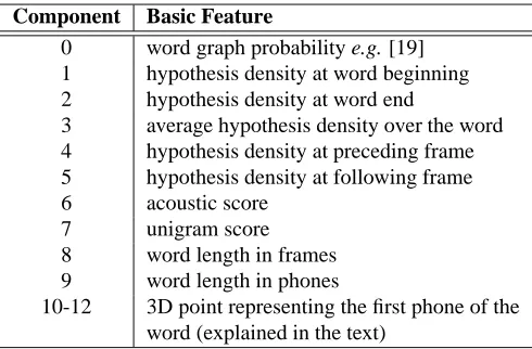
We use a fairly standard set of confidence features augmented with one novel feature to form a feature vector for each hypothesized word. Since our boosting classifier will ignore components that supply spurious information, there is no harm in including as many features as possible (other than wasted processing time). Our basic set of features is listed in Table 1.

2 3 BOOSTING CLASSIFIER

Component Basic Feature

0 word graph probability e.g. [19] 1 hypothesis density at word beginning 2 hypothesis density at word end

3 average hypothesis density over the word 4 hypothesis density at preceding frame 5 hypothesis density at following frame 6 acoustic score

7 unigram score 8 word length in frames 9 word length in phones

10-12 3D point representing the first phone of the word (explained in the text)

Table 1: Core feature set used to construct the feature vector for each hypothesized word. This vector is augmented by left and right context as described in the text.

the Viterbi search sense) preceding and following words. Our final confidence feature vector thus has dimension 39.

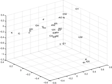
Our one novel feature is a 3D representation of the first phone of each word. Our motivation is that we wish to include more information about the intrinsic confusabil-ity of words in confidence scoring metrics. However, since there is no simple low-dimensional monothetic representation of word confusability, we approximate it by the confusability of the first phone of the word. This is reasonable since an error at the beginning of the word will impact the whole word. Indeed, many words begin with easily confusible consonants.

We represent the confusability of the first phone in the word by transforming the phone label to a real three-dimensional point using Multi-dimensional scaling (MDS). This transformation from a label to the real space allows us to treat this feature nu-merically, similar to all other features. MDS (e.g. [20]) is a standard technique which transforms a series of objects, about which only relative distance information is avail-able, to a series of -dimensional points. The mapping attempts to preserve the relative

distances between objects such that objects which are known to be ‘close’ to each other are ‘close’ in the dimensional space. To transform phone labels using MDS, we use

a phone confusion matrix as a measure of the relative distance among them. Figure 1 shows our 3D representation of TIMIT phones derived using MDS on their confusion matrix. We see that linguistic categories are well preserved in this Euclidean space. We use this mapping to obtain a 3D point for the first phone of each word.

3

Boosting Classifier

3.1 Choice of Weak Learner 3 −0.6 −0.4 −0.2 0 0.2 0.4 0.6 0.8 −0.6 −0.4 −0.2 0 0.2 0.4 −1.2 −1 −0.8 −0.6 −0.4 −0.2 0 0.2 0.4 ER R IH UW OY N OW EY Y AO NG AY AE AH AA ZH EH UH AW CH F TH V DH HH D T G K

Figure 1: 3D Euclidean representation of TIMIT phones derived using MDS on their confusion matrix. For clarity, only points close to the origin are shown.

algorithms were introduced by Schapire [13] and Freund [6].

Boosting applies a classification procedure iteratively to a set of weighted data vec-tors. At first each vector is assigned an equal weight (or a weight depending on its prior probability). On each iteration, a classifier is learnt and the vectors that are classified incorrectly have their weights increased while those that are correctly classified have their weights decreased. The intuition is that vectors which are difficult to classify receive more attention on subsequent iterations.

The classifier learnt at each iteration is called a ‘weak’ classifier. It is called weak because it is not expected to classify the training data very well, only better than 50%. Typically a very simple weak classifier is used. The final classifier, the so-called ‘strong’ classifier, is formed as a weighted sum of the weak classifiers learnt at each step. Table 2 gives a algorithmic description of the boosting classification procedure.

The formal guarantees provided by boosting classification theory are quite strong. Freund and Schapire prove that the training error of the strong classifier approaches zero exponentially in the number of iterations.

3.1

Choice of Weak Learner

compo-4 3 BOOSTING CLASSIFIER

Begin with training vectors and their associated labels where for

negative and positive examples respectively.

Initialize weights "! for

#$% respectively, where& and' are the

number of negatives and positives respectively.

For()*++%+,.- :

1. Normalize the weights,

0/132

0/1 465

"78 /1

so that0/ is a probability distribution and adds up to+ .

2. For each feature, 9 , train a classifier which is restricted to using a single

feature. The error is evaluated with respect to /,:

4

;< =1?>@"<.

3. Choose the classifier,$/ , with the lowest error: /.

4. Update the weights:

/=A88B /1DC FEHGJI

/

where KLMN if example is classified correctly, KLOP otherwise, and C / QDR

E QR

.

The final strong classifier is:

8 =ST U 4WV /=78SX /J/ =SY 46V /=78HX / otherwise whereX /Z6[]\^ _ R

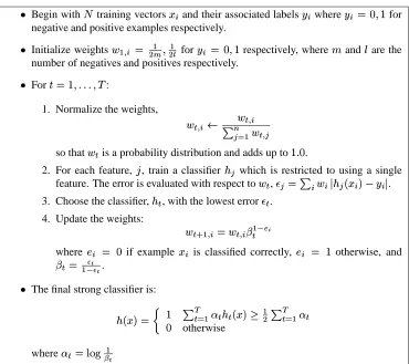
Table 2: The boosting algorithm for learning a classifier. - weak classifiers are

con-structed. The final strong classifier is a weighted linear combination of the- weak

classifiers where the weights are inversely proportional to the training errors.

nent ` , a threshold a , and a directionb indicating the direction of the inequality

sign.

T

U

ifb ` dceb a otherwise

(1)

In practice no single feature component can perform the classification task with low error. Typically the first weak learner has an error rate of about$+f and the final learners

closer to$+hg . Figure 2 shows weak and strong learner error rates for the HUB496 data

5

0 20 40 60 80 100 120 140 160 180 200 0.15

0.2 0.25 0.3 0.35 0.4 0.45 0.5

Iteration Number

Error Rate

Weak Learner Strong Learner

Figure 2: Strong and weak error rates as a function of the number of iterations in the boosting algorithm. The dataset was a subset of the HUB4 confidence set.

4

Alternative Classifiers

In addition to boosting, we also experiment with alternative classifiers on our feature set. We use standard implementations of Support Vector Machines (SVM) [2] and Classification and Regression trees (CART) [1].

5

Experimental Results

We test our algorithm on confidence features obtained from two data sets. The first set is the 1996 HUB4 test set [3], a total of about 3 hours of speech. The second set is sampled from around 9 hours of transcribed Web Broadcast News from our internal

SpeechBot test set [10].

To obtain lattices from which our confidence features are extracted, we run a stan-dard HMM-based decoder built on the HUB496 and HUB497 training sets. For the

SpeechBot test set, the training data is Real-Audio encoded and decoded to account for

the streamed nature of the test set. The decoder for the HUB4 data uses 16 Gaussian mixture components per state. For the Speechbot data, 8 mixture components are used. The word error rates for the data sets are 32.9% and 55.0% respectively.

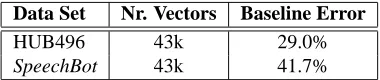
Using the decoded word lattices, We construct confidence feature vectors as de-scribed in Section 2 for each word in the top hypothesis. Each feature is labeled with ‘1’ or ‘0’, reflecting whether or not the word is correct. Table 3 gives further details of the feature sets, including the baseline error or prior probability of Class 0. Notice that the error rates for the confidence vectors are not the same as the recognizer error rates. This is because deleted words, which count as errors for word error rate scores, do not appear in confidence feature sets (since there is no word to obtain features for).

Data Set Nr. Vectors Baseline Error

HUB496 43k 29.0%

SpeechBot 43k 41.7%

6 6 DISCUSSION

For all the experiments reported in this paper we perform cross validation. The data sets were randomized and split into 10 different sets. Training was performed on 9 sets and testing on the remaining set. This experiment was repeated 10 times by testing on all 10 sets. Our error rates are therefore averages over all 10 sets. This experimental method provides more accurate and valid results.

We also report the confidence error rates for both classes. Any classifier can be tuned to minimize global error rate or to minimize false positives or false negatives. In this paper we tune our classifiers to operate close to the equal error rate point where both false positives and false negatives are similar. Otherwise, our results will be biased by the prior probabilities of each class.

5.1

HUB496 results

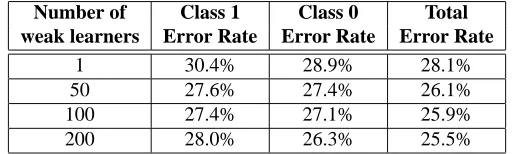
Table 4 shows the results of tests on the HUB4 dataset. We show error rates for boosting systems with up to 200 weak learners. We did not observe significant improvements beyond this number. The results show that we can reduce the error rate toigj+hgk , an

improvement ofli$+mnk relative to the baseline ofio+k .

Number of Class 1 Class 0 Total

weak learners Error Rate Error Rate Error Rate

1 30.4% 28.9% 28.1%

50 27.6% 27.4% 26.1%

100 27.4% 27.1% 25.9%

200 28.0% 26.3% 25.5%

Table 4: Error rates for the HUB4 96 data set and their relationship to the number of weak learners.

On this set, the CART classifier produces an error rate of iop+mnk , almost no

im-provement over the baseline. The SVM classifier yields an error rate off+hik , again

no improvement.

5.2

SpeechBot results

Table 5 presents results for the Speechbot dataset. Again, we show error rates for up to 200 weak learners. A substantial improvement over the baseline result is observed. We improve the error rate fromq+srk toitr+utk , a relative improvement offf+pk . On this

dataset, the CART classifier produces an error rate ofiop$+qk and the SVM classifier an

error rate offtij+utk .

6

Discussion

7

Number of Class 1 Class 0 Total

weak learners Error Rate Error Rate Error Rate

1 28.6% 34.4% 31.9%

50 26.1% 29.7% 28.2%

100 25.5% 29.2% 27.7%

200 25.7% 28.9% 27.6%

Table 5: Error rates for the SpeechBot data set and their relationship to the number of weak learners.

0 5 10 15 20 25 30

0 5 10 15

Weak Learner

Percentage of weight

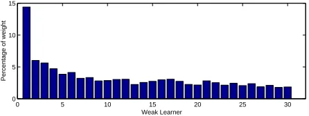
Figure 3: Weights applied to each of the weak learners. The first five learners contribute close to 25% to the decision.

Because our choice of weak learner is a dimension specific classifier, it is inter-esting to examine when each feature component is chosen by the boosting iterative procedure. Intuitively, confidence vector features that are chosen early are more

infor-mative than those chosen later on. Using this simple analysis we observe that features

f , , f , , r and are the first six features chosen by the strong classifier. These

features correspond to the average hypothesis density over the word, the word graph probability, the hypothesis density at the word beginning, the unigram score and the middle component of our 3D representation of the first phone in the word. This order of feature choice is relatively consistent across experiments and datasets. Interestingly, our 3D phone representation is more informative than many of the other lattice-derived features.

Figure 3 displays typical weights applied to the first thirty weak learners. We ob-serve that the features for context words (from components 14 to 39) that provide an-other 26 components to our 39 dimensional vector only appear after position 10 or so. In fact, after learningl weak learners onlyiu out of the possiblef are chosen. This

8 REFERENCES

7

Conclusion

In this paper we have explored the use of boosting techniques for confidence scoring. We have compared them with two other classification schemes, CART and SVMs, and consistently outperformed them. Our choice of boosting algorithm offers several advantages. It is simple to implement, fast in its learning time, and very flexible in the choice of weak learner. In this paper we have used a very simple learner that picks individual features and classifies them with a threshold and a flag indicating the direction of the inequality sign. Remarkably, such a simple classifier is able to provide up to afoqk improvement in performance on the SpeechBot dataset. More sophisticated

weak learners such as CART should be able to improve this performance at the cost of longer training time.

In the future we will explore how confidence scores can be used to improve our public audio indexing system, both to refine the retrieval function as well as for lan-guage and acoustic model adaptation. Confidence scores will allow us to effectively mine more than hours of unlabeled audio currently indexed by the SpeechBot

system.

8

Acknowledgments

We thank Michael Jones and Paul Viola for their help and support in this research. We also thank Jean-Manuel Van Thong for providing us with phonetic confusion matrices.

References

[1] L. Breiman, J.H. Friedman, R.A. Olshen, and C.J.Stone. Classification and

Re-gression Trees. Chapman & Hall, New York, 1984.

[2] Christopher Burges. A Tutorial on Support Vector Machines for Pattern Recog-nition. Data Mining and Knowledge Discovery, 2(2), 1998.

[3] Linguistic Data Consortium. 1996 English Broadcast News Dev and Eval.

http://www.ldc.upenn.edu, 1996.

[4] S. Cox and S. Dasmahapatra. A semantically-based confidence measure for speech recognition. In Proc. ICSLP, 2000.

[5] S. Cox and R. Rose. Confidence measures for the switchboard database. In Proc.

ICASSP, 1996.

[6] Yoav Freund and Robert E. Schapire. A decisitheoretic generalization of on-line learning and an application to boosting. In Computational Learning Theory:

Eurocolt ’95, pages 23–37. Springer-Verlag, 1995.

REFERENCES 9

[8] T. Kemp and T. Schaaf. Estimating confidences using word lattices. In Proc.

EUROSPEECH, 1997.

[9] T. Kemp and A. Waibel. Unsupervised training of a speech recognizer: recent experiments. In Proc. EUROSPEECH, 1999.

[10] B. Logan, P. Moreno, J.-M. Van Thong, and E. Whittaker. An experimental study of an audio indexing system for the Web. In Proc. ICSLP, 1996.

[11] C. Pai, P. Schmid, and J. Glass. Confidence scoring for speech understanding systems. In Proc. ICSLP, 2000.

[12] T. Schaaf and T. Kemp. Confidence measure for spontaneous speech recognition. In Proc. ICASSP, 1997.

[13] Robert E. Schapire. The strength of weak learnability. Machine Learning,

5(2):197–227, 1990.

[14] M.-H. Siu, H. Gish, and F. Richardson. Improved estimation, evaluation and applications of confidence measures for speech recognition. In Proc.

EU-ROSPEECH, 1997.

[15] K. Tieu and P. Viola. Boosting image retrieval. In International Conference on

Computer Vision, 2000.

[16] C. Uhrik and W. Ward. Confidence metrics based on n-gram language model backoff behaviors. In Proc. EUROSPEECH, 1997.

[17] M. Weintraub, F. Beaufays, Z. Rivlin, Y. Konig, and A. Stolcke. Neural - network based measures of confidence for word recognition. In Proc. ICASSP, 1997. [18] A. Wendemuth, G. Rose, and J. G. A. Dolfing. Advances in confidence measures

for large vocabulary. In Proc. ICSLP, 2000.

[19] F. Wessel, K. Macherey, and R. Schlueter. Using word probabilities as confidence measures. In Proc. ICASSP, 1998.

[20] F. W. Young and R. M. Hamer. Multidimensional Scaling: History, Theory and

CRL

2001/08

J

uly

2001

A

Boosting

Appr

oac

h

for

Confidence

Scoring

P

edro

J

.

Moreno

,

Beth

Logan

and

Bhiksha