An Experimental and Theoretical Study of Active Flow Control

(1)

Study of Active Flow Control

Thesis by Damian George Hirsch

In Partial Fulfillment of the Requirements for the Degree of

Doctor of Philosophy

CALIFORNIA INSTITUTE OF TECHNOLOGY Pasadena, California

2017

(2)

(3)

Knowing is not enough; we must apply. Being

willing is not enough; we must do.

(4)

Abstract

The accelerating growth of environmental awareness has not stopped at the aerospace industry. The need for greener and more efficient airplanes threatens to outpace the flow of new technology. This has ignited development in several fields, one of which is active flow control (AFC). Active flow control has quickly proven its tremendous potential for real applications. Even though the roots of this technology date back a century, we still lack fundamental understanding. This thesis combines both modern and traditional approaches to lay out a new foundation for future research.

The thesis first focuses on the rising stars of active flow control: the so-called fluidic oscillators or sweeping jet actuators. These devices consist of simple, rigid internal geometries that create a sweeping output jet motion. The fluid dynamic interactions with the internal geometry are studied in detail using high-speed Schlieren imaging. Additionally, the influence of adjacent sweeping jets is investigated. It is revealed that the internal driving mechanism is far stronger than the fluid dynamic interactions at the outlet, resulting in a completely independent jet behavior.

Next, a high-lift airfoil design is combined with active flow control, and an extensive wind tunnel study is carried out. It is shown that for the given wing design active flow control leads to much higher lift benefits when applied to the trailing edge. Applied to the leading edge active flow control disrupts the vortex lift of the high-lift airfoil, resulting in a deleterious lift effect; however, it shows potential for pitch moment control. This project also underlines the advantages of jet-like active flow control over steady blowing actuation at limited available mass flow rates.

The momentum input coefficient as an important parameter in active flow control is discussed in detail, identifying common misconceptions and difficulties that hinder its proper calculation. An innovative, much simpler approach is introduced. This allows a detailed study of the underlying physics, unveiling unknown limitations of active flow control. The approach is then used as a model to derive the novel concept of thermal active flow control. Experimental studies, including a wind tunnel test campaign, are performed to confirm the viability of the concept for practical applications.

(5)

(6)

Acknowledgements

First of all, I would like to express my gratitude to my advisor, Professor Mory Gharib, for giving me the opportunity to work on an exciting and fulfilling research project. I would like to thank him for his inspiring guidance, invaluable support, comprehensive understanding, and great trust over the last few years. I am also grateful to the members of my thesis committee, namely Professors Hans Hornung, Joseph Shepherd, and Tim Colonius, for the encouraging discussions and resourcefulness advice. A special thanks goes to my last committee member Professor Israel Wygnanski for his tremendous mentorship and collaboration.

I thank the entire Gharib research group members for all the scientific and non-scientific discussions: Chris Roh, Morgane Grivel, Cong Wang, Nathan Martin, Jinglin Huang, Cecilia Huertas-Cerdeira, Chris Dougherty, Marcel Veismann, Sean Mendoza, Emilio Graff, David Jeon, Francisco Pereira, David Kremmers, and Masoud Beizaie. In particular, I want to thank Stephanie Rider and Manuel Bedrossian for their help throughout my PhD and for enduring me in the same office for such a long time. I would also like to thank Martha Salcedo, Peggy Blue, Christine Ramirez, and Dimity Nelson for their priceless administrative support. A big thanks goes to Ali Kiani, Matavos Zargarian, and Joe Haggerty for creating usable parts out of my impossible drawings. I am also grateful to all visiting students who worked with me in the Lucas Wind Tunnel: Yann Glauser, Damien Fulliquet, Justin Mercier, Mark Vujicic, Albéric Gros, Nicolas Bosson, and Raimondo Pictet.

I would like to acknowledge Boeing for their financial support of my research throughout my entire time at Caltech, as well as Northrop Grumman for their funding during my second and third year.

Among my friends, I would like to especially thank Phillipe Tosi, Nicholas Burali, Kazuki Maeda, Georgios Rigas, Oliver Schmidt, Christian Kettenbeil, Thibaud Talon, Ryan McMullen, Rich Ken-nedy, Ian Brownstein, and Silvio Tödtli for their morale support and for keeping me a responsible human being these last few years.

(7)

List of Illustrations

Number Page

1.1 Airbus A320 family with only small differences between tail sizes.. . . 1

1.2 Conceptual design of a sweeping jet actuator. . . 5

2.1 Examples of other uses of fluidic oscillators. . . 8

2.2 Sweeping jet sandwiched between two optical glass plates visualized in a Schlieren setup. . . 9

2.3 Startup flow and first oscillation of a sweeping jet actuator. . . 10

2.4 Creation of vortices during the sweeping cycle. . . 11

2.5 Transition to sonic exit jet and reduction of sweep angle. . . 12

2.6 Sonic exit jet at higher flow rate with increased frequency and large reduction of sweep angle. . . 13

2.7 Underexpanded jet at a high inlet to outlet pressure ratio. . . 13

3.1 Bench-top model setup. . . 15

3.2 Definition of the deflection angle for the top (θ1) and bottom (θ2) sweeping jet actuator. The spacing between the actuators is labeled withd. . . 16

3.3 Detection of the jets using the Canny edge detection method.. . . 16

3.4 Reduction of the detection area significantly improves the accuracy of the center of mass calculation (dots). . . 17

3.5 Illustration of the two in-sync states of the jets. . . 18

3.6 Typical FFT of a sweeping jet actuator with its jet frequency clearly dominating. The first harmonic is very weak while the second harmonic is a bit stronger. There is also another frequency that is slightly stronger than the first harmonic frequency that is most likely connected with the pressure source that runs the experimental setup. . . 21

3.7 FFT of the phase looks exactly like the FFT of the jet deflection angles. However, a closer look at the plot reveals a second peak which corresponds to the frequency of the second jet. . . 24

(10)

3.9 FFT of the Hilbert transform. . . 26

3.10 Mass flow distribution for a standard sweeping jet with an opening angle of 100◦. . . 28

4.1 The Northrop wing model with its dimensions in inches. The full-span wing has roughly a chord of 25 inches and a span of 50 inches resulting in a semi-span aspect ratio of 2. . . 31

4.2 LAVLET airfoil shape with circled AFC locations at 1%, 10%, and 80% of chord. . 31

4.3 Fairing to provide a smooth aerodynamic transition from the tunnel floor to the model root.. . . 32

4.4 Sweeping jet actuator plate (top) and steady blowing plate (bottom). . . 32

4.5 Schematic of leading edge design showing actuator arrays, gaskets, actuator clamps, plenums, and outer mold line (OML) covers for the 1% and 10% slot. . . 33

4.6 Schematic of trailing edge design showing actuator arrays, gaskets, actuator clamps, plenums, and outer mold line (OML) covers for the 80% slot. . . 33

4.7 Reduced span configuration with only two spanwise sections. The span was reduced to limit the high amplitude oscillations caused by the flexible force balance. The dashed line represents the mean rotation line about which the pitch moment is measured (body coordinates). . . 34

4.8 Spanwise pressure tap locations on the reduced span wing. . . 35

4.9 Omega FMA-2621A Mass Flow Controllers mounted beneath the test section regulate the mass flow rate into each bank of actuators. . . 35

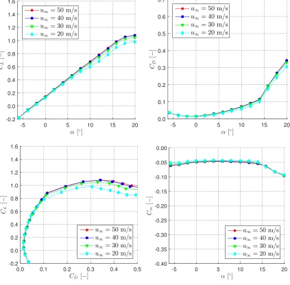
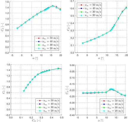
4.10 Comparison between the baselines of the two basic configurations with flap deflections δF=0◦andδF=45◦. . . 37

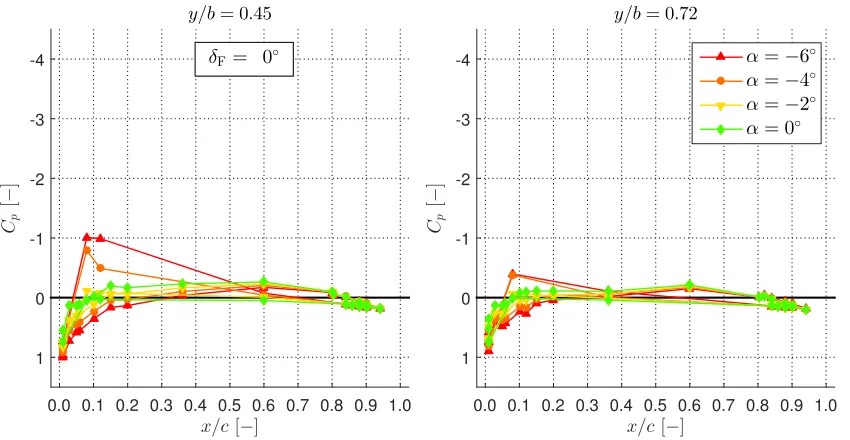
4.11 Pressure distributionCpwithδF=0◦for angles: -6◦, -4◦, -2◦, and 0◦. . . 39

4.12 Pressure distributionCpwithδF=0◦for angles: 2◦, 4◦, 6◦, and 8◦. . . 39

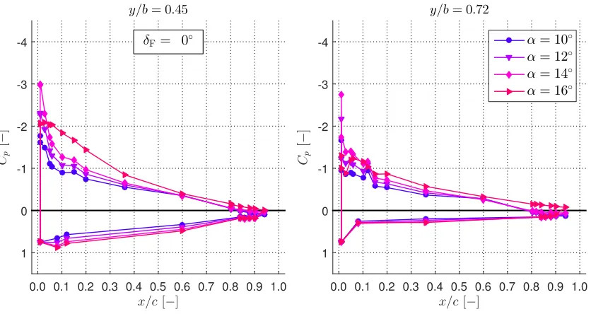
4.13 Pressure distributionCpwithδF=0◦for angles: 10◦, 12◦, 14◦, and 16◦. . . 40

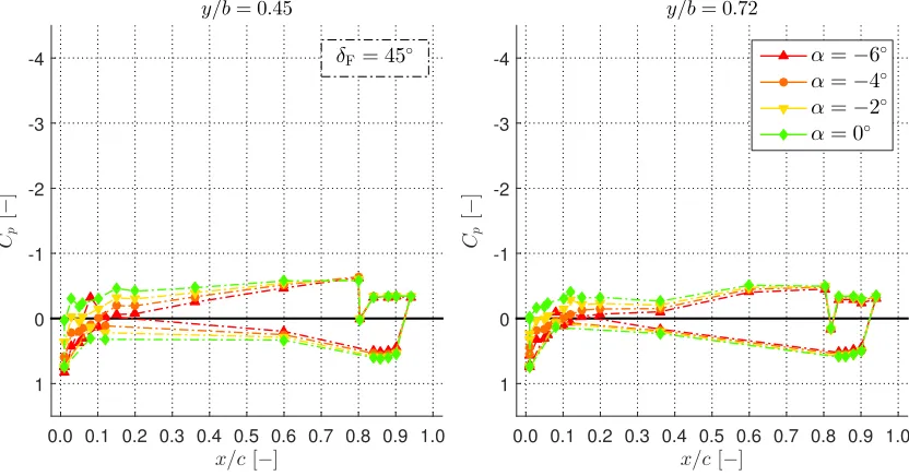
4.14 Pressure distributionCpwithδF=45◦for angles: -6◦, -4◦, -2◦, and 0◦. . . 41

4.15 Pressure distributionC_pwithδF=45◦for angles: 2◦, 4◦, 6◦, and 8◦. . . 42

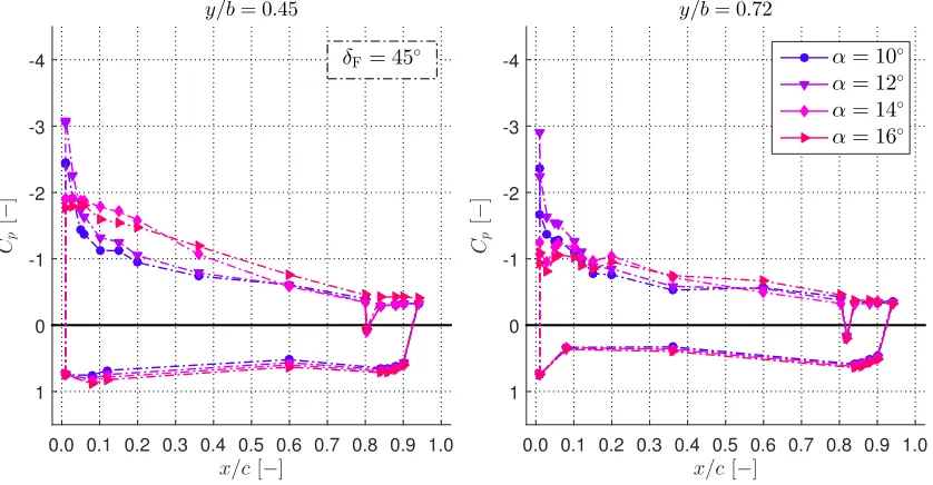
4.16 Pressure distributionC_pwithδF=45◦for angles: 10◦, 12◦, 14◦, and 16◦. . . 42

4.17 Reynolds independence for the non-deflected flapδF=0◦. . . 44

(11)

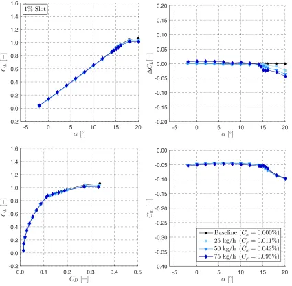
4.19 Impact of steady blowing withδF=0◦at the 1% slot with increasing mass flow rates

compared to the baseline case (no blowing).. . . 46 4.20 Comparison of pressure distributionCpforδF=0◦with steady blowing from the 1%

slot at a mass flow rate of 75 kg/h. Baseline (no blowing) is a dashed line, while the

solid line represents the blowing case. Angles: -2◦, 0◦, 2◦, 4◦. . . 47 4.21 Comparison of pressure distributionCpforδF=0◦with steady blowing from the 1%

solid line represents the blowing case. Angles: 6◦, 8◦, 10◦, 12◦. . . 48 4.22 Comparison of pressure distributionCpforδF=0◦with steady blowing from the 1%

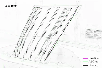
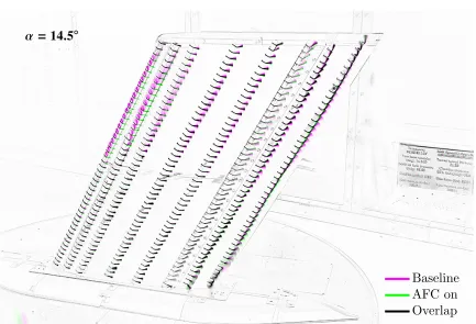
solid line represents the blowing case. Angles: 14◦, 16◦, 18◦, 20◦. . . 48 4.23 Tuft visualization forδF = 0◦ with steady blowing from the 1% slot at a mass flow

rate of 75 kg/h andα=10◦. . . 49 4.24 Tuft visualization forδF = 0◦ with steady blowing from the 1% slot at a mass flow

rate of 75 kg/h andα=14.5◦. . . 49 4.25 Impact of steady blowing with δF = 0◦ at the 10% slot with increasing mass flow

rates compared to the baseline case (no blowing). . . 51 4.26 Comparison of pressure distributionC_p for δF = 0◦ with steady blowing from the

10% slot at a mass flow rate of 75 kg/h. Baseline (no blowing) is a dashed line, while

the solid line represents the blowing case. Angles: -2◦, 0◦, 2◦, 4◦. . . 52 4.27 Comparison of pressure distributionCp for δF = 0◦ with steady blowing from the

the solid line represents the blowing case. Angles: 6◦, 8◦, 10◦, 12◦. . . 52 4.28 Comparison of pressure distributionCp for δF = 0◦ with steady blowing from the

the solid line represents the blowing case. Angles: 14◦, 16◦, 18◦, 20◦. . . 53 4.29 Tuft visualization forδF =0◦with steady blowing from the 10% slot at a mass flow

rate of 75 kg/h andα=10◦. . . 53 4.30 Tuft visualization forδF =0◦with steady blowing from the 10% slot at a mass flow

(12)

4.31 Impact of steady blowing with δF = 0◦ at the 80% slot with increasing mass flow

rates compared to the baseline case (no blowing). . . 55 4.32 Comparison of pressure distributionCp for δF = 0◦ with steady blowing from the

the solid line represents the blowing case. Angles: -2◦, 0◦, 2◦, 4◦. . . 56 4.33 Comparison of pressure distributionCp for δF = 0◦ with steady blowing from the

the solid line represents the blowing case. Angles: 6◦, 8◦, 10◦, 12◦. . . 56 4.34 Comparison of pressure distributionCp for δF = 0◦ with steady blowing from the

the solid line represents the blowing case. Angles: 14◦, 16◦, 18◦, 20◦. . . 57 4.35 Tuft visualization forδF =0◦with steady blowing from the 80% slot at a mass flow

rate of 75 kg/h andα=10◦. . . 57 4.36 Tuft visualization forδF =0◦with steady blowing from the 80% slot at a mass flow

rate of 75 kg/h andα=14.5◦. . . 58 4.37 Impact of steady blowing with δF = 45◦ at the 1% slot with increasing mass flow

rates compared to the baseline case (no blowing). . . 59 4.38 Comparison of pressure distributionC_p for δF = 45◦with steady blowing from the

the solid line represents the blowing case. Angles: -6◦, -4◦, -2◦, 0◦. . . 60 4.39 Comparison of pressure distributionCp for δF = 45◦with steady blowing from the

the solid line represents the blowing case. Angles: 2◦, 4◦, 6◦, 8◦. . . 60 4.40 Comparison of pressure distributionCp for δF = 45◦with steady blowing from the

the solid line represents the blowing case. Angles: 10◦, 11◦, 12◦, 14◦. . . 61 4.41 Tuft visualization forδF =45◦ with steady blowing from the 1% slot at a mass flow

rate of 75 kg/h andα=8◦.. . . 61 4.42 Tuft visualization forδF =45◦ with steady blowing from the 1% slot at a mass flow

(13)

4.43 Impact of steady blowing withδF = 45◦at the 10% slot with increasing mass flow

rates compared to the baseline case (no blowing). . . 63 4.44 Comparison of pressure distributionCp for δF = 45◦with steady blowing from the

the solid line represents the blowing case. Angles: 10◦, 11◦, 12◦, 14◦. . . 65 4.47 Tuft visualization forδF=45◦with steady blowing from the 10% slot at a mass flow

rate of 75 kg/h andα=8◦.. . . 65 4.48 Tuft visualization forδF=45◦with steady blowing from the 10% slot at a mass flow

rate of 75 kg/h andα=12.5◦. . . 66 4.49 Impact of steady blowing withδF = 45◦at the 80% slot with increasing mass flow

rates compared to the baseline case (no blowing). . . 67 4.50 Comparison of pressure distributionC_p for δF = 45◦with steady blowing from the

the solid line represents the blowing case. Angles: 10◦, 11◦, 12◦, 14◦. . . 69 4.53 Tuft visualization forδF=45◦with steady blowing from the 80% slot at a mass flow

rate of 75 kg/h andα=8◦.. . . 69 4.54 Tuft visualization forδF=45◦with steady blowing from the 80% slot at a mass flow

(14)

4.55 Impact of sweeping jet actuators with δF = 0◦ at the 1% slot with increasing mass

flow rates compared to the baseline case (no blowing). . . 71 4.56 Comparison of pressure distributionCpforδF=0◦with sweeping jet actuators from

the 1% slot at a mass flow rate of 50 kg/h. Baseline (no blowing) is a dashed line,

while the solid line represents the blowing case. Angles: -2◦, 0◦, 2◦, 4◦. . . 72 4.57 Comparison of pressure distributionCpforδF=0◦with sweeping jet actuators from

while the solid line represents the blowing case. Angles: 6◦, 8◦, 10◦, 12◦. . . 72 4.58 Comparison of pressure distributionCpforδF=0◦with sweeping jet actuators from

while the solid line represents the blowing case. Angles: 14◦, 16◦, 18◦, 20◦.. . . 73 4.59 Tuft visualization forδF=0◦with sweeping jet actuators from the 1% slot at a mass

flow rate of 75 kg/h andα=10◦. . . 74 4.60 Tuft visualization forδF=0◦with sweeping jet actuators from the 1% slot at a mass

flow rate of 75 kg/h andα=14.5◦. . . 74 4.61 Impact of sweeping jet actuators withδF =0◦at the 10% slot with increasing mass

flow rates compared to the baseline case (no blowing). . . 75 4.62 Comparison of pressure distributionC_pforδF=0◦with sweeping jet actuators from

(15)

4.67 Impact of sweeping jet actuators withδF =0◦at the 80% slot with increasing mass

flow rates compared to the baseline case (no blowing). . . 79 4.68 Comparison of pressure distributionCpforδF=0◦with sweeping jet actuators from

flow rate of 75 kg/h andα=14.5◦. . . 82 4.73 Tuft visualization forδF=0◦with sweeping jet actuators from the 80% slot at a mass

flow rate of 75 kg/h andα=16◦. . . 83 4.74 Impact of sweeping jet actuators withδF =45◦at the 1% slot with increasing mass

flow rates compared to the baseline case (no blowing). . . 84 4.75 Comparison of pressure distribution Cp for δF = 45◦ with sweeping jet actuators

from the 1% slot at a mass flow rate of 75 kg/h. Baseline (no blowing) is a dashed

line, while the solid line represents the blowing case. Angles: -2◦, 0◦, 2◦, 4◦. . . 85 4.76 Comparison of pressure distribution Cp for δF = 45◦ with sweeping jet actuators

line, while the solid line represents the blowing case. Angles: 6◦, 8◦, 10◦, 11◦. . . . 85 4.77 Comparison of pressure distribution Cp for δF = 45◦ with sweeping jet actuators

line, while the solid line represents the blowing case. Angles: 12◦, 14◦, 16◦, 18◦. . . 86 4.78 Tuft visualization forδF=45◦with sweeping jet actuators from the 1% slot at a mass

(16)

4.79 Tuft visualization forδF=45◦with sweeping jet actuators from the 1% slot at a mass

flow rate of 75 kg/h andα=12.5◦. . . 87 4.80 Impact of sweeping jet actuators withδF=45◦at the 10% slot with increasing mass

line, while the solid line represents the blowing case. Angles: 6◦, 8◦, 10◦, 11◦. . . . 89 4.83 Comparison of pressure distribution C_p for δF = 45◦ with sweeping jet actuators

line, while the solid line represents the blowing case. Angles: 12◦, 14◦, 16◦, 18◦. . . 90 4.84 Tuft visualization for δF = 45◦ with sweeping jet actuators from the 10% slot at a

mass flow rate of 75 kg/h andα=8◦. . . 90 4.85 Tuft visualization for δF = 45◦ with sweeping jet actuators from the 10% slot at a

mass flow rate of 75 kg/h andα=12.5◦. . . 91 4.86 Impact of sweeping jet actuators withδF=45◦at the 80% slot with increasing mass

line, while the solid line represents the blowing case. Angles: 6◦, 8◦, 10◦, 11◦. . . . 93 4.89 Comparison of pressure distribution Cp for δF = 45◦ with sweeping jet actuators

line, while the solid line represents the blowing case. Angles: 12◦, 14◦, 16◦, 18◦. . . 94 4.90 Tuft visualization for δF = 45◦ with sweeping jet actuators from the 80% slot at a

(17)

4.91 Tuft visualization for δF = 45◦ with sweeping jet actuators from the 80% slot at a

mass flow rate of 75 kg/h andα=10◦. . . 95 4.92 Tuft visualization for δF = 45◦ with sweeping jet actuators from the 80% slot at a

mass flow rate of 75 kg/h andα=12.5◦. . . 95 4.93 Comparison of sweeping jet actuators with δF = 45◦ at different slots including a

case with all slots active. The fully active case is a combination of the single slots

effects. There is no combinatory benefit. . . 97 4.94 The power coefficientCΠis plotted against the flow coefficientCQ. It is evident that

an open slot (steady blowing) does not require a much lower power to run due to the

plumbing resistance and the introduction of a choke plate. . . 99 5.1 Comparison between the different Cµ calculations and their errors compared to a

compressible approach. The operational region represents typical mass flow rate

values that were used in actual experiments. . . 106 5.2 The relation betweenCµandCQshows three different flow states (left), and reveals a

physical limitation of values that can be achieved at fixed freestream conditions (right).107 5.3 The three different flow states can be observed in the Schlieren images as well. . . . 108 6.1 TheCµ-model introduced in Section 5.3 confirms the theoretical derivation predicting

a reduced mass flow rate at higher temperatures to achieve the same momentum

coefficients (left). Thermal effects also allow breaching into the “non-reachable

zone” from Fig. 5.2b (right). . . 111 6.2 The bench-top model for the thermal active flow control concept study is designed to

withstand high temperatures. . . 112 6.3 Comparison between the classic Cµ model predictions and the total momentum

coefficientCJ. . . 114 6.4 Comparison between the uncorrected CJ-model and the adjusted model with the

discharge coefficient (Cd≈0.7) for the straight jet. . . 115 6.5 Vertical tail model seen from the suction side. The actuator covers were removed to

(18)

6.7 Normalized lift coefficient C_L0 versus coefficient of mass flow rate input C_Q: the

heated cases indeed show a higher performance benefit compared to the baseline case

for all freestream velocities but seem to underperform compared to theory. . . 119 6.8 Normalized lift coefficient C_L0 versus momentum coefficient Cµ: the heated input

momentum coefficientCµshows a lower benefit compared to its cold equivalent. The

equationCµ,hot=Cµ,colddoesn’t seem to hold. . . 120 6.9 The pressure ratios P show a plateauing effect once the flow is choked in the jet

nozzle as predicted by theory. With these values the effective temperature of the air

can be calculated based on Eq. (6.20). The results of this calculation are summarized

in Table 6.1. . . 121 6.10 The normalized lift coefficientC_L0 and the temperature-corrected momentum

coeffi-cientCµcollapse on top of each other proving thatCµ,hotyields the same lift benefits

at a lower mass flow rate than its cold equivalentCµ,cold. . . 123 7.1 Two cases where Cµ fails to collapse the data. The first case happens when the

freestream velocityu∞is changed (left). On the right the second case is illustrated

where the actuator nozzle area differs. . . 125 7.2 The normalized lift coefficient C_L0 plotted against the input momentum coefficient

C_µfor different jet types exemplifyC_µ’s weakness of not collapsing data at different

freestream velocities. As shown in Fig. 7.1, it also fails to collapse the different

actuator types even at the same freestream velocities. . . 127 7.3 IfCµ is calculated in an incompressible fashion (which is wrong) the data collapses

for different freestream velocities unlike when it’s calculated the appropriate way.

Nevertheless, the incompressible momentum coefficient still fails to collapse the

different actuator areas. . . 128 7.4 Plotting the normalized lift coefficientC_L0 against the flow coefficientCQreveals the

connection to an incompressibleCµ calculation. CQ is able to collapse the data for

different freestream velocities, but yet is still not able to collapse different actuator

(19)

7.5 Velocity ratio for the different actuator types. A certain velocity ratio is needed before

any beneficial effects start to occur. The minimum velocity ratio is independent of the

freestream velocity within the same type of actuator, but different for each actuator

type. . . 130 7.6 Velocity ratio multiplied by the area ratio scales the values in the separate cases

compared to the pure velocity ratio. However, because the actuators all have different

actuator areas the combined plot changes. The two sweeping jet actuators are now

much closer to each other and the steady blowing case also reduced its difference. . 131 7.7 The mass flux shows an expected similarity with the velocity ratio at low jet velocities.

However, at high velocities (with compressibility effects) it is able to keep the data

collapsed. There is also no cut-off value anymore when the nozzle chokes. The

interplay between the velocity ratio for the scaling and the density ratio to take care

of the compressibility effects leads to this great result. . . 132 7.8 The net momentum coefficientCµ,nethas a vanishing effect compared to the standard

momentum coefficientCµ. The results look practically identical to Fig. 7.2 . . . 134 7.9 The combination of flow coefficientCQ and velocity ratioujet/u∞ leads to the net

flow coefficientCQ,netthat is able to collapse different freestream velocities as well

as vastly different actuator designs. . . 135 7.10 The net flow coefficientCQ,netis not able to account for thermal active flow control. 136 7.11 Adjusting the net flow coefficient by the square root of the temperature ratio leads to

the extended mass flow coefficientMthat is now able to collapse the thermal active

flow control data. . . 137 7.12 Illustration of the PIV setup on the vertical tail. On the left, one can see the spanwise

location of the laser sheet between actuators 17 and 18 (counted from the root). The

top view on the right shows the camera’s field of view marked by the red box. This

region is of particular interest as it covers the actuators on the left side and spans over

(20)

7.13 On the left, the measured lift and extended mass flow coefficient values during the

PIV experiment are shown. The vertical line represents a change of slope in the

lift curve, and the different circle colors correspond to different data sets shown in

Figs. 7.14 and 7.15. On the right, the PIV baseline (no actuation) is shown where the

contour colors correspond to the velocity magnitude normalized by the freestream

velocity. The black lines with arrows show the streamlines and -directions. The dark

gray area corresponds to the lower part of the flap. . . 139 7.14 PIV images from the non-linear part of the extended mass flow coefficientM. The

strong non-linear increase is shown here to be the removal of the separation region

caused by an entrainment effect of the created shear layer between the high-velocity

jet and the much slower flow in the recirculation zone. . . 140 7.15 PIV images from the linear part of the extended mass flow coefficient M after the

separation is removed. The increasing lift is generated by an increased velocity close

to the flap surface due to the jet’s additional mass flow in that region. The accelerated

flow causes a lower overall pressure on the flap surface, pulling the streamline closer

to the flap surface. This leads to an increased circulation around the entire vertical

tail (supercirculation), and is essential responsible for the lift benefits. . . 141 7.16 The different “states” in AFC can be described by boundary layer thickening,

separa-tion control, and supercirculasepara-tion. The extended flow coefficientMis capable of not

(21)

List of Tables

Number Page

3.1 Calculated frequency of the different jet cases. The maximum deviation from the

reference case is less than 0.35% suggesting that there is no change in frequency due

to any possible interaction of the actuators. . . 22 3.2 Calculated frequency of the different jet cases using a Fourier fit and comparison to

the FFT approach. The approaches get to similar results with a maximum deviation

of 0.08%. . . 23 3.3 FFT of the phase angle reveals two peaks for each of the jet frequencies.. . . 23 3.4 Comparison between the frequency difference calculated by an FFT of the angle

deflection versus the Hilbert transform. . . 26 3.5 FFT of the deflection angle at a reduced mass flow rate of 3 kg/h per jet.. . . 27 6.1 Calculation of the effective temperature ratios based on the pressure ratios

(22)

Nomenclature

Acronyms

AFC Active Flow Control

AFRL Air Force Research Laboratory

AHLLE Advanced High Lift Leading Edge

BL Boundary Layer

CFD Computational Fluid Dynamics

DDPIV Defocusing Digital Particle Image Velocimetry

ERA Environmentally Responsible Aviation

FFT Fast Fourier Transform

LAVLET Laminar Airfoil Virtual Leading Edge Technology

LE Leading Edge

MAC Mean Aerodynamic Chord

MOLEC Multi-Objective Leading Edge Concept

NACA National Advisory Committee for Aeronautics

NASA National Aeronautics and Space Administration

OML Outer Mold Line

PIV Particle Image Velocimetry

TAFC Thermal Active Flow Control

TE Trailing Edge

(23)

Greek Symbols

α Angle of attack [ ° ]

δF Flap deflection angle [ ° ]

ε Relative error [ - ]

η System efficiency [ - ]

γ Heat capacity ratio [ - ]

Λ Leading edge sweep [ ° ]

ν Kinematic viscosity [m2/s]

ω Angular frequency [rad/s]

φ Phase angle [ ° ]

Π Power [W]

ρ Density [kg/m3]

θ Jet deflection angle [ ° ]

Roman Symbols

A Area [m2]

a Speed of sound [m/s]

AF Axial force measure by balance [N]

AR Aspect ratio [ - ]

b Wing span [m]

c Wing chord [m]

(24)

CΠ Power coefficient [ - ]

CD Drag coefficient [ - ]

C_d Discharge coefficient [ - ]

cf Relative flap chord [ - ]

CJ Total momentum coefficient [ - ]

CL Lift coefficient [ - ]

Cm Pitching moment coefficient [ - ]

C_p Pressure coefficient [ - ]

cp Heat capacity at constant pressure [J/(kg·K)]

C_Q Flow input coefficient [ - ]

cv Heat capacity at constant volume [J/(kg·K)]

d Actuator spacing [m]

F Force [N]

f Frequency [Hz]

h Specific enthalpy [J/kg]

L Lift force [N]

M Mach number [ - ]

Û

m Mass flow rate [kg/s]

n Number of actuators [ - ]

p Pressure [Pa]

(25)

Û

Q Volume flow rate [m3/s]

R Specific gas constant [J/(kg·K)]

Rec Chord Reynolds number [ - ]

S Planform area [m2_]

SF Side force measure by balance [N]

T Temperature [K]

u Fluid velocity in the x or freestream direction [m/s]

v Fluid velocity in the y-direction [m/s]

x Coordinate or distance [m]

y Coordinate or distance [m]

Superscripts

0 _Normalized

Subscripts

0 Zero mass flow rate input

∞ Freestream

ac Aerdodynamic center

act Actuator

atm Atmospheric

bal Balance

c Calibration value

(26)

cold Value at the lower temperature

crit Critical value

e Effective value

hot Value at the higher temperature

i Induced

jet Value at the jet exit of an AFC device

m Measured value

min Minimum required value

net Velocity-corrected value

ref Reference

s Static

sup Supply

t Total

Other Symbols

A Actuator area ratio [ - ]

M Extended mass flow coefficient [ - ]

P Pressure ratio [ - ]

S Spacing ratio [ - ]

T Temperature ratio [ - ]

V Velocity magnitude divided by freestream velocity [ - ]

(27)

Cµ = 1mujetÛ

2ρ∞u

2

∞S

CΠ =

γ

γ−1p∞mÛ

"

_psup

p∞

γ−1_γ

−1

#

1

2ρ

2

∞u3∞S

C_D= SF sin1α−AF cosα

2ρ∞u∞S2 =

D 1

2ρ∞u2∞S

CL = SF cos1α+AF sinα

2ρ∞u

2

∞S =

L 1

2ρ∞u

2 ∞S

Cm= PM1+L(xac−xbal)

2ρ∞u∞Sc2

Cp = p

−p∞

1

2ρ∞u∞2

CQ = _ρ∞u∞SmÛ = ρs

Û Q ρ∞u∞S

(28)

C h a p t e r 1

Introduction

1.1 Motivation

Commercial airlines spend billions of dollars on jet fuel every year. If one can offer new ways to save millions of gallons of jet fuel, the airlines’ attention is practically guaranteed. Tighter environmental regulations and higher fuel prices will further accelerate this process in the near future. Yet even the coming generation of new commercial airplane models will, within a few years, inevitably struggle to meet these criteria. The accelerating growth of environmental awareness threatens to outpace the flow of new technology. In response, NASA’s Environmentally Responsible Aviation (ERA) Project aimed to increase the technology advancement’s pace and set it to fast-track the introduction of several “green” developments that have been tested since 2009 (Norris, 2014).

As one of many other technologies developed and tested under the ERA Project, one particular research objective focused on the size of the vertical tail. As of today, its size is determined by the eventuality of losing an engine during takeoff or landing while being exposed to strong crosswinds. Yet the vertical tail is a large surface that is barely used during nominal flight conditions. On top of that, manufacturing constraints still lead to a family of airplanes sharing the same vertical tail, sized for the shortest body and forcing the longer planes to carry unnecessarily large tails (Seele, Graff, Lin, et al., 2013). This is well visualized in Fig. 1.1, where the Airbus 320 family shows

Figure 1.1:Airbus A320 family with only small differences between tail sizes.

(29)

enhance the performance of a vertical tail to reduce its size in future designs. A smaller vertical tail would lead to a reduction of weight and drag of an airplane, which can improve fuel efficiency and aerodynamic performance. The ERA project also demonstrated that the concept does not only work in a laboratory environment, such as the Lucas Wind Tunnel at Caltech, but also at full-scale at the NASA Ames wind tunnel. Most recently in 2015, Boeing took it a step further and tested the technology on a real, full-sized Boeing 757 airplane called the ecoDemonstrator 757. It was concluded that this technology has the potential to make a big impact on commercial airplanes, and that there could be a significant change to airplane design.

Extensive research on this topic was performed during the early discoveries of active flow control in the 1950s and early 1960s, when the technology was tested on wings of military aircraft, mainly to reduce their takeoff and landing speed. Examples are the Grumman F9F-4 Panther Jet, the Lockheed T2V-1 Seastar U.S. Navy Jet Trainer, and the U.S.A.F. Lockheed F104 Starfighter among many others. Most of the current understanding and theory of AFC is from that time. However, the traditional theory presents itself with a variety of inconsistencies and unsolved questions, such as “[...] a favorable Reynolds number effect [...] was experienced during the flight tests” (Attinello, 1961). This phenomenon could also be observed during the ERA project comparing data between the Lucas Wind Tunnel model and the NASA Ames model. Conclusively, there is still a significant lack of fundamental fluid dynamic understanding that hasn’t been resolved for over half a century.

1.2 Study Objectives

(30)

coefficientCµ, are not able to cover the whole spectrum of active flow control and fail in certain situations. If these two major issues can be resolved, the industry would be more willing to adapt current airplane models with AFC. The long-term goal should be to increase the fundamental under-standing to a point where a new generation of airplanes would be built from scratch, incorporating AFC at the start of the design process. This would certainly trigger another revolution in the aircraft industry in terms of effectiveness and possibilities. Airplanes would most likely look completely different compared to today’s design, which has not evolved much over the last couple of decades.

Several specific objectives have been formulated as a guidance for this thesis and are described as follows:

(a) Gain insight into the internal flow structure of sweeping jets, one of the currently most popular active flow control devices. Investigate the interaction between adjacent sweeping jets with the absence of freestream flow.

(b) Combine the effects of a high-lift airfoil and active flow control. Identify the importance of the flow control location along the chord of a wing, and compare different actuation devices.

(c) Elucidate the problems with the input momentum coefficientCµ, simplify its calculation, and understand its underlying mechanisms.

(d) Investigate the concept of thermal active flow control (TAFC).

(e) Derive a new similarity parameter to replace the flawed momentum input coefficientCµ.

1.3 Scope of Study

(31)

surface, and many more. Active flow control require energy expenditure. From a control standpoint of view active flow control can be divided further into open-loop and closed-loop active flow control. Closed-loop active flow control defines all techniques that make use of a control loop to manipulate the flow. As a consequence, these techniques usually require a sensor to gather information of the current flow state as well as a processing unit to calculate the next manipulation steps. Open-loop active flow control can be defined as techniques that do not make us of a control loop. Thus, they do not require sensing and processing of data. However, they usually can be turned on, off, and often have intermediate settings. Examples of open-loop active flow control methods include steady suction or blowing, the use of synthetic jets, and of course unsteady suction and blowing. The techniques described in this thesis are part of the latter with some use of steady blowing as comparison. All used techniques are part of the open-loop active flow control subgroup but will further be referred to as active flow control or AFC.

The modern use of flow control was certainly pioneered by Ludwig Prandtl during his Nobel-prize-worthy presentation at the Third Congress of Mathematicians at Heidelberg, Germany in 1904. His paper“Über Flüssigkeitsbewegung bei sehr kleiner Reibung”, which translates to "On Fluid Motion at Very Small Friction”, introduced the boundary-layer theory in just eight pages (as required for acceptance by the congress). By applying his theory to flow separation, he was able to clearly explain the concept of stall for the first time. This opened the way for understanding the motion of real fluids and fueled the research in aerodynamics for the next three decades. Stimulated by political tension during the years 1940 to 1970, flow control research accelerated even more. Flow control played a major role to achieve the military needs for the development of fast, highly maneuverable, efficient aircraft, missiles, ships, submarines, and torpedoes. Natural laminar flow, laminar flow control, and polymer drag reduction were discovered during this era. The years 1970-1990 were dominated by the energy crises and brought a noticeable shift of interest from the military to the civilian sector. The appearance of the first inexpensive computers supported the development of more complex flow control devices such as the reduction of skin-friction drag in turbulent boundary layers. Since the 1990s more complex control devices have been pursued (Gad-el-Hak, 2007).

(32)

sweeping jet actuators, proved themselves as an attractive option because they have no moving parts and are believed to be highly efficient AFC devices. However, they do require a steady supply of compressed air, and in this regard, they resemble steady blowing although they use less air. A schematic drawing of a typical modern actuator used as an AFC device is shown inSection 1.3.

Figure 1.2:Conceptual design of a sweeping jet actuator.1

Sweeping jet actuators were used in aeronautical experiments for the purpose of delaying separation on airfoils (Seele, Tewes, et al., 2009;Phillips, Woszidlo, and Wygnanski, 2010;Desalvo, E. Whalen, and Glezer, 2012) and on wings (Tewes, Taubert, and Wygnanski, 2010). The usefulness of these devices prompted the need to understand their working principle (Vatsa, Koklu, and Wygnanski, 2012) and their effect on boundary layers that are about to separate from the surface. In the interim one may improve the efficiency of these actuators for a specific application by using dimensional analysis that enables one to determine the leading parameters controlling the process (Woszidlo and Wygnanski, 2011;Woszidlo, Nawroth, et al., 2010). They also found application as drag-reduction devices on trucks (Seifert, Stalnov, et al., 2008) and as active combustion control devices (Guyot, Paschereit, and Raghu, 2009).

Next, Rathay et al., 2014 applied synthetic jet actuators, also called zero-net-mass-flux (ZNMF) actuators, to a typical vertical stabilizer of a commercial airplane model. Their actuators were placed in a linear array next to the hinge of the rudder for the purpose of attaching the flow over the rudder surface at large rudder deflection angles, thereby increasing its effectiveness. Seele, Graff, Gharib, et al., 2012andSeele, Graff, Lin, et al., 2013discuss recent significant findings of active flow control on a typical vertical stabilizer. The former paper focuses on sweeping jet actuation that was applied directly to the rudder, while the later evaluates the effects of actuation from the trailing

(33)

edge of the main element. Both show that sweeping jets can provide significant improvements in lift and drag with minimal input. Smaller jets spaced farther apart make better use of air unless extreme gains are required. This so called “air fence effect” or “fluidic fence effect” at high actuator spacings could prove useful to increase the sweep angle of wings while delaying tip stall at low speed (Graff and Wygnanski, 2014). The scope of this study is to build onto these recent results employed on the vertical tail and to improve their predictability.

1.4 Thesis Outline

Chapter 2 investigates the working principle of sweeping jet actuators via high-speed Schlieren

imaging. It discusses their unique characteristics and tries to connect the findings to the promising performance as an AFC device.

Chapter 3discusses the interaction between two adjacent sweeping jet actuators without an

over-laying crossflow. The jet positions are tracked visually and then analyzed using FFT. The spacing between the actuators was varied and two different input pressures were compared. The tracked data also allowed to plot the mass distribution of a sweeping jet actuator for these two different cases.

Chapter 4explores the use of active flow control on a high-lift airfoil design. The interaction between

the virtual leading edge of the airfoil and the active flow control is exemplified. Additionally, this chapter analyzes the effects of different chordwise flow control locations and possible combinatory effects. It also compares the traditional steady blowing actuation with the more modern use of sweeping jets. This comparison eventually leads to the discussions inChapter 7.

Chapter 5 is dedicated to the importance of the momentum input coefficient C_µ in the area of

active flow control. Furthermore, the chapter tries to properly define Cµ and point out common problems and misconceptions. A simplification of its calculation is introduced, which will be used as a baseline in the following chapters.

Chapter 6 introduces Thermal Active Flow Control (TAFC). The chapter derives the concept

mathematically, and proceeds with a bench-top experiment to get a practical proof of concept. In a last step, TAFC is applied to a vertical tail model and its effects on lift performance are studied.

Chapter 7debunks the weaknesses ofCµ and proceeds with the identification of key variables that

(34)

applied to different AFC actuation devices to show the new parameter’s superior characteristics. Lastly, the parameter is extended to account for TAFC.

Chapter 8summarizes the results of this thesis. Their implications on future work and possible

(35)

C h a p t e r 2

An Investigation of Sweeping Jets

Sweeping jets play an important role in recent AFC research as they seem to be more efficient in terms of lift generation compared to other actuator types. They were born as fluidic analogs of electronics components at the Harry Diamond Labs in the 1950’s. As such they found few applications, though the thrust reverser actuator system of both the DC-10 and the Concorde employed fluidic operational amplifiers. An example of an amplifier is shown inFig. 2.1a; small amounts of flow in the control ports C1and C2divert the main jet, thus increasing the flow rate (“current”) in the desired output port.

Vented outputs can also be used to amplify “voltage” (pressure). Many geometries self-oscillate when the control ports are not connected, and this type of oscillator has found its way into shower

(a)Example of a fluidic amplifier.2

(b)Flow meter using self-oscillation to convert flow rate to frequency.3

Figure 2.1:Examples of other uses of fluidic oscillators.

(36)

heads, paint sprayers, and wind shield wiper nozzles. InFig. 2.1ban implementation of a flow meter which uses the self-oscillation to convert flow rate to frequency is illustrated.

In order to visualize the internal and external flow of a sweeping jet actuator, several transparent models were built to be used in a Schlieren setup. Fig. 2.2shows a model made with optical glass sandwiching aluminum parts which form the sweeping jet actuator. The vertical line in the image represents the edge of the glass plates, and the entire geometry is quasi two-dimensional with a thickness of 0.1 inches, a jet throat width of 0.2 inches, and an opening angle of 100◦. At lower speeds the jet is visualized by a temperature difference using cold gas (tetrafluoroethane) in the air hose but eventually pressure differences are sufficient.

Figure 2.2:Sweeping jet sandwiched between two optical glass plates visualized in a Schlieren setup.

(37)

fluid to one feedback passage than the other (here the upper one). In Fig. 2.3f, oscillations have now begun; the internal jet has flipped from one side to the other, attaching itself to one of the solid surfaces (“islets”) forming the main cavity of the actuator. The feedback passages are now fed by

(a) (b)

(c) (d)

(e) (f)

Figure 2.3:Startup flow and first oscillation of a sweeping jet actuator.

(38)

fact, many previous experiments were carried out using rectangular actuators as described by (Lucas et al., 2008). The whole geometry could be made slightly asymmetric and it would then oscillate in a “syncopated” fashion. However, all the sweeping jet actuators in this thesis were carefully built with the intention of making them symmetric.

(a) (b)

(c) (d)

(e) (f)

Figure 2.4:Creation of vortices during the sweeping cycle.

(39)

(see Section 3.3.6). When the vortex leaves the exit trapezoid, which corresponds to a transition from a quasi two-dimensional space to a three-dimensional space, it immediately interacts with the ambient air and rapidly dissipates (Fig. 2.4d). While the dissipation of the previous vortex is still ongoing, the jet starts to separate itself from the wall again. This downward motion now creates a counterclockwise-rotating vortex (Fig. 2.4e). This newly created vortex is now pulled downwards with the sweeping motion and the whole process repeats (Fig. 2.4f). These vortices significantly enhance the mixing capabilities of the sweeping jets. It is believed that these distinct characteristics play a major role in the sweeping jets’ promising performances in AFC applications.

As the pressure continues to increase the outlet jet reaches the speed of sound (Fig. 2.5a), and the first signs of shocks appear. In its subsonic state the jet fully attaches to the exit walls and creates the vortices before the jet switches sides. As the back pressure further increases the now sonic jet stays no longer attached to the walls and reduces its sweeping angle (Figs. 2.5bto2.5d).

(a) (b)

(c) (d)

Figure 2.5:Transition to sonic exit jet and reduction of sweep angle.

(40)

(a) (b)

Figure 2.6:Sonic exit jet at higher flow rate with increased frequency and large reduction of sweep angle.

Fig. 2.7ais at the maximum pressure ratio (about 6) between the inlet and outlet (ambient) the given setup is able to provide. The outlet jet is now underexpanded, and this allows it to reattach to the side walls. InFig. 2.7b one can see circular black stripes that emit from the center of the jet exit. These stripes represent sound waves created by the jet noise. At this condition, the sweeping jets can be extremely loud to a point where the sound waves are getting visible in Schlieren.

(a) (b)

(41)

C h a p t e r 3

The Influence of Adjacent Sweeping Jets

3.1 Introduction

(42)

3.2 Experimental Setup

To answer some of these questions a bench-top model was built where the distance between two adjacent sweeping jet actuators could easily be changed. The experimental setup is shown in Fig. 3.1a. Actuators can be freely moved along a slot to change their respective spacing and more

(a)Bench-top model to study the influence of adjacent jets on each other depending on the separation distance. The swee-ping jets actuators are colored in blue.

(b)Single sweeping jet ac-tuator that was used for the experiment.

Figure 3.1:Bench-top model setup.

(43)

Figure 3.2:Definition of the deflection angle for the top (θ1) and bottom (θ2) sweeping jet actuator. The

spacing between the actuators is labeled withd.

It was believed, that any influence the actuators exhibit would translate into a position or frequency adjustments of one or even both jets to accommodate the presence of the other. To put “position” into an actual quantitative value, it was decided to record the jet deflection angles of the actuators as defined inFig. 3.2. To extract the angle deflectionsθ1andθ2from the images an algorithm was

written to track the jets and calculate their respective deflection angles. The images were analyzed using an edge detection method introduced byCanny, 1986. The method calculates the gradient of

(a)Raw image (b)Processed image

(c)Overlay

(44)

an intensity image using the derivative of a Gaussian filter. This method applies two thresholds to the gradient: a high threshold for low edge sensitivity and a low threshold for high edge sensitivity. It starts with the low sensitivity result and then grows it to include connected edge pixels from the high sensitivity result. This helps fill in gaps in the detected edges and makes the Canny method less likely to be fooled by noise compared to other methods and more likely to detect true weak edges. InFig. 3.3one can see a comparison between a raw image, the processed version, and an overlay of both. It’s evident that this method is fully capable of tracking the jets without much difficulty. However, the main interest is acquiring the deflection angle and not tracking the jets themselves. A simple way to do so is by calculating the center of mass of the tracked pixels of the processed image (3.3b). This is more difficult than it sounds because the large wake region that has already mixed well with the surrounding air lags considerably behind the actual jet deflection angle. Fig. 3.4a

(a)Full detection area with inaccurate center of mass cal-culation (dot).

(b)Detection area limited to a narrow band right after the jet.

Figure 3.4:Reduction of the detection area significantly improves the accuracy of the center of mass calcu-lation (dots).

(45)

The first images taken showed that two adjacent sweeping jet actuators went through cycles with three distinguishable states: parallel-sync, crossed-sync, and async. These states are defined as:

parallel-sync: θ1 = θ2, (3.1)

cross-sync: θ1 =−θ2, (3.2)

async: θ1 , θ2. (3.3)

Parallel-sync is a parallel motion of the jet with respect to each other, while cross-sync means the jets are mirrored along the horizontal center line resulting in a criss-cross behavior. Async describes all the other jet orientations where the jets are in a random orientation to each other. The two in-sync states are illustrated inFig. 3.5.

(a)Parallel-sync:θ₁=θ₂ (b)Cross-sync:θ₁=−θ₂

Figure 3.5:Illustration of the two in-sync states of the jets.

3.3 Results and Discussion

(46)

Thus, the spacing ratioSdefined as the ratio between the jet exit trapezoidal width (1 inch) and jet spacingd lies between 0 and 3.5 covering the case of approximately 2 for the real models.

There are three distinct ways to evaluate the adjacent actuators’ influence:

Cross-Correlation: The cross-correlation between two signals in the original time-domain is

calculated with this method. In this case, either the time dependent jet deflection angles between two jets of the same recordingθ1 andθ2 or the same jet for two different recordings at different

spacing can be evaluated. If there is an interaction between two actuators, the former can give insight into a time-dependent dependence as the correlation value is expected to change with increasing time-shifts (assuming windows are used to get rid of edge effects). The latter would reveal if there is a change to the correlation over the whole time-domain by changing the distance between two jets. It would be expected that the correlation coefficients stay the same if there is no interaction between the actuators.

Unfortunately, this technique has a few major drawbacks. First, the signal of the jet angles is oscillating, which means that a correlation would also be an oscillating “signal” with values between -1 and 1. One could either average the results for comparison or focus on the maximum and minimum correlations values only. However, the much bigger drawback is that cross-correlation relies on a clean signal. The tracked images of the jet recordings can’t live up to that due to noise in tracking, varying supply-pressure, and tiny geometry differences between the two actuators. These issues cause small frequency differences between the actuators on the order of 1%, which is sufficient to prevent any success with this approach.

Frequency Domain: Here the signals are converted into the frequency domain using a Fast Fourier

(47)

a work-around: it is possible to look at the frequency domain of the phase time-domain signal. The phase angleφis defined as

φ=θ1−θ2. (3.4)

If one looks at the frequency domain of the phase angle, one would now expect to see changes even if two adjacent actuators are in a parallel-sync or cross-sync state.

Hilbert Transform: Another interesting technique is to convert the time-domain signal into an

analytic signal via the Hilbert transform. This transforms the signal into a vector of complex numbers. The angle deflection which are of sinusoidal form will be converted into complex numbers whose magnitudes are constant and whose phase is changing with the original sinusoidal wave. Thus, this technique allows one to get the instantaneous phase lag between two signals. The major limitation of this approach is that the signal needs to be mono-component, which means that the signal of interest needs to dominate the recording. Any substantial interference must be filtered out.

3.3.1 FFT of a Single Jet and Comparison to Reference

First, a Fast Fourier Transform is taken for the reference jet and every jet spacing. A typical FFT that was acquired for all the cases is shown inFig. 3.6. The frequency of the jet is clearly dominating the amplitude. The next higher peak corresponds to the second harmonic of the jet frequency. The first harmonic of the jet frequency is very weak and barely visible. A possible reason might be that right next to it there is another peak from an unknown source. This peak is also visible for the reference jet, and hence it is not an interaction frequency. It might have to do with the pressure source that runs the experimental setup, meaning it could be connected to the compressor’s RPM.

(48)

0 1000 2000 3000 4000

Frequency [Hz]

0 0.05 0.1 0.15 0.2 0.25

A

m

p

li

tu

d

e

[r

ad

2

/H

z]

1st _Harmonic

2nd _Harmonic

Jet Frequency

Figure 3.6:Typical FFT of a sweeping jet actuator with its jet frequency clearly dominating. The first harmonic is very weak while the second harmonic is a bit stronger. There is also another frequency that is slightly stronger than the first harmonic frequency that is most likely connected with the pressure source that runs the experimental setup.

3.3.2 Comparison of the FFT Results to a Fourier Type Fit

To verify that the FFT from the previous section calculates the correct frequencies, a different approach can be used that was not mentioned in the introductory part. Because the jet deflection angle follows approximately a sinusoidal wave over time, it is possible to fit the data to a sine function where the angular frequencyωis directly linked to the jet frequency f. A simple sine function as fit seemed to be a little too simple and wouldn’t have given enough degrees of freedom to acquire a good result. Thus, it was decided to use a first-order Fourier series

f(a0,a1,b1, ω,x)=a0+a1cos(ωx)+b1sin(ωx) (3.5)

(49)

Table 3.1:Calculated frequency of the different jet cases. The maximum deviation from the reference case is less than 0.35% suggesting that there is no change in frequency due to any possible interaction of the actuators.

S[-] Jet Frequency [Hz] Difference [Hz] Deviation [%]

Reference 1249.4 -

-0.000 1248.0 -1.4 0.11

0.125 1253.5 4.1 0.33

0.250 1248.0 -1.4 0.11

0.375 1248.0 -1.4 0.11

0.500 1252.4 3.0 0.24

0.625 1247.5 -1.9 0.15

0.750 1251.1 1.7 0.14

0.875 1249.1 -0.3 0.02

1.000 1251.1 1.7 0.14

1.125 1253.3 3.9 0.31

1.250 1250.2 0.8 0.06

1.500 1248.0 -1.4 0.11

1.750 1250.2 0.8 0.14

2.000 1248.0 -1.4 0.06

2.250 1248.0 -1.4 0.11

2.500 1248.0 -1.4 0.11

2.750 1246.9 -2.5 0.20

3.000 1248.0 -1.4 0.11

3.250 1246.9 -2.5 0.20

3.500 1246.9 -2.5 0.20

images each. In general it can be stated that both methods have an outstanding agreement, and that there is a large confidence in the results including the drawn conclusion that there is no evidence for any actuator interaction.

3.3.3 FFT of Phase Angle

(50)

Table 3.2:Calculated frequency of the different jet cases using a Fourier fit and comparison to the FFT approach. The approaches get to similar results with a maximum deviation of 0.08%.

S[-] Fourier Fit [Hz] FFT [Hz] Difference [Hz] Deviation [%]

Reference 1248.4 1249.4 -1.0 0.08

0.000 1249.0 1248.0 1.0 0.08

0.125 1253.5 1253.5 0.0 0.00

0.250 1248.0 1248.0 0.0 0.00

0.375 1248.0 1248.0 0.0 0.00

0.500 1252.4 1252.4 0.0 0.00

0.625 1247.6 1247.5 0.1 0.01

0.750 1251.2 1251.1 0.1 0.01

0.875 1249.2 1249.1 0.1 0.01

1.000 1251.2 1251.1 0.1 0.01

1.125 1253.3 1253.3 0.0 0.00

1.250 1250.2 1250.2 0.0 0.00

1.500 1247.6 1248.0 -0.4 0.03 1.750 1249.9 1250.2 -0.3 0.02

2.000 1248.2 1248.0 0.2 0.02

2.250 1248.4 1248.0 0.4 0.03

2.500 1248.4 1248.0 0.4 0.03

2.750 1247.3 1246.9 0.4 0.03

3.000 1247.9 1248.0 -0.1 0.01

3.250 1247.2 1246.9 0.3 0.02

3.500 1247.4 1246.9 0.5 0.04

the jets don’t seem to have any influence on each other; they are completely independent of each other. Table 3.3shows that the FFT of the phase indeed unveils the separate jet frequencies when

Table 3.3: FFT of the phase angle reveals two peaks for each of the jet frequencies.

S[-]

Jet 1 Jet 2

FFT Angle [Hz] FFT Phase [Hz] FFT Angle[Hz] FFT Phase [Hz]

0.000 1248.0 1248.0 1256.6 1256.6

0.125 1253.5 1253.5 1262.9 1262.9

0.250 1248.0 1248.0 1261.0 1261.0

0.375 1248.0 1248.0 1264.0 1263.7

0.500 1252.4 1252.4 1263.2 1263.2

0.625 1247.5 1247.5 1256.3 1256.3

0.750 1251.1 1250.0 1262.3 1262.3

0.875 1249.1 1249.1 1258.8 1258.8

1.000 1251.1 1251.1 1263.7 1263.7

1.125 1253.3 1253.3 1265.1 1264.8

1.250 1250.2 1250.2 1261.0 1260.4

(51)

0 1000 2000 3000 4000

Frequency [Hz]

0 0.05 0.1 0.15 0.2 0.25

A

m

p

li

tu

d

e

[r

ad

2

/H

z]

1st _Harmonic

2nd _Harmonic

Jet Frequency

(a)FFT of the phase angle.

1100 1150 1200 1250 1300 1350 1400 1450

Frequency [Hz] 0

0.05 0.1 0.15 0.2 0.25

A

m

p

li

tu

d

e

[r

ad

2 /H

z]

Frequency Jet 1

Frequency Jet 2

(b)Zoom: Two peaks are distinguishable.

(52)

deflection angle even though the phase signal is much noisier in the frequency domain (creates wider peaks). This is also the reason why a few small differences can be observed when comparing direct deflection to phase angle FFT.

3.3.4 Hilbert Transform of Phase Angle

To support the previous results a Hilbert transform of the phase angles was performed. Because the phase is used again, this technique is limited to the cases with two observable jets. Fig. 3.8 summarizes the phase lags for the different spacing ratios. The phase lag continuously increases

0 0.5 1 1.5 2 2.5

t [s]

-5 0 5 10 15 20 25 30 35 40

P

h

a

se

C

y

cl

es

[#

]

S _{= 0} .000 S _{= 0}

.125 S _{= 0}

.250 S _{= 0}

.375 S _{= 0}

.500 S _{= 0}

.625 S _{= 0}

.750 S _{= 0}

.875 S _{= 1}

.000 S _{= 1}

.125 S _{= 1}

.250

Figure 3.8:Hilbert transform of the phase angle. A continuously increasing phase lag can be observed for all the signals.

(53)

Table 3.4:Comparison between the frequency difference calculated by an FFT of the angle deflection versus the Hilbert transform.

S[-] ∆fFFT[Hz] ∆fHilbert[Hz]

0.000 8.6 8.9 0.125 9.4 10.4 0.250 13.0 12.8 0.375 16.0 15.4 0.500 10.8 10.6 0.625 8.8 9.3 0.750 11.2 11.3 0.875 9.7 10.2 1.000 12.6 12.8 1.125 11.8 12.0 1.250 10.8 9.2

underlying frequencies are around 1250 Hz. An FFT of the Hilbert transform will again result in the same frequency results, but the distinct frequencies of the two jets are now smeared out (Fig. 3.9).

0 1000 2000 3000 4000

Frequency [Hz]

0 0.2 0.4 0.6 0.8 1

A

m

p

li

tu

d

e

[r

ad

2

/H

z]

Jet Frequencies

1st _Harmonics

Figure 3.9:FFT of the Hilbert transform.

3.3.5 Reduction of Mass Flow Rate

An Experimental and Theoretical Study of Active Flow Control

Study of Active Flow Control

Abstract

Acknowledgements

Table of Contents

List of Illustrations

List of Tables

Nomenclature

Introduction

An Investigation of Sweeping Jets

The Influence of Adjacent Sweeping Jets

Frequency [Hz]

A

m

p

li

tu

d

e

[r

ad

/H

z]

Frequency [Hz]

A

m

p

li

tu

d

e

[r

ad

/H

z]

Frequency [Hz]

A

m

p

li

tu

d

e

[r

ad

/H

z]