EFFECT OF FATIGUE ON SSVEP DURING VIRTUAL WHEELCHAIR NAVIGATION

A HYBRID AND NOVEL OPTIMIZATION FRAMEWORK

FOR DENOISING AND CLASSIFICATION OF MEDICAL

IMAGES USING DTCWP AND NEURO-FUZZY CLASSIFIERS

1_{A.VELAYUDHAM,} 2_R.KANTHAVEL, 3_{K.MADHAN KUMAR}

1_{Assistant Professor (SG), Department of IT, Cape Institute of Technology, Levengipuram-627114, India}

2_{Professor and Head, Department of ECE, Velammal Engineering College, Chennai-66, India}

3_{Associate Professor, Department of ECE, PET Engineering College, Vallioor-627117, India}

E-mail: [email protected], [email protected], [email protected]

ABSTRACT

Computed tomography (CT) images are usually corrupted by several noises from the measurement process complicating the automatic feature extraction and analysis of clinical data. To attain the best possible diagnosis it is very vital that medical images be clear, sharp, and free of noise and artifacts. In this research paper, we propose a robust technique to denoise, detect and classify the tumour part from CT medical images. Our proposed approach consists of four phases, such as denoising, region segmentation, feature extraction and classification. In the denoising phase Dual Tree Complex Wavelet Packets and Empirical Mode Decomposition are used for removing noise. Here, histon process is used in order to surmount the smoothing filter type and it will not affect the lower dimensions. We have taken into consideration two noises, Gaussian and salt & pepper for proposed technique. The performance of the proposed technique is assessed on the five CT images for the parameters, PSNR and SDME. In the segmentation process K-means clustering technique is employed. For the feature extraction, the parameters contrast, energy and gain are extracted. In classification, a modified technique called Cuckoo-Neuro Fuzzy (CNF) algorithm is developed and applied for detection of the tumour region. The cuckoo search algorithm is employed for training the neural network and the fuzzy rules are generated according to the weights of the training sets. Then, classification is done based on the fuzzy rules generated. From the obtained outcomes, we can conclude that the proposed denoising technique have shown better values for the SDME of 69.9798 and PSNR of 25.4193 for salt & pepper noise which is very superior compared to existing methods. Moreover our proposed technique has shown an accuracy of 96.3% which is very better than the existing methods.

Keywords: CT, EMD, DTCWP, PSNR, SDME, CNF, Contrast, Energy, Entropy, K-Means, Sensitivity, Specificity, Accuracy

1. INTRODUCTION

Denoising of medical images like X-RAY, CT, MRI, PET and SPECT encompass diminutive information about heart, brain, nerves and more which leads physician for precise analysis [14] of diseases. In the case of CT, numerous mathematical and medical applications [12, 13] can be applied to conclude whether the normal tissue has been infected by the mutations of the cancer cell. Recent wavelet thresholding based denoising methods have proved capable, during the conservation of the high frequency signal details [3]. The threshold at certain scale is a constant for all wavelet coefficients in standard wavelet thresholding based noise reduction methods [16]. Fundamentally, the noisy image is transformed into the wavelet domain, then the

image segmentation as the quantity of clusters is

generally identified for images of particular regions of the human anatomy. A number of experimenters have launched associated investigations into K-means clustering segmentation. Though a significant and noteworthy advancement has been made in this regard, still there is greater

computational intricacy and the need for

superfluous software functionality [21]. Clustering programs, like k-means and ISODATA, function in an unsupervised mode and have been performed on an extensive domain of categorization dilemmas [22]. For categorizing the tumour segments, physical classification tends to lead to manual flaws, in addition to relying heavily on person to person, protracted and elongated runtime along with

non-reproducible outcomes. Therefore, an

automatic or semi-automatic classification

technique is the need of the hour as it tends to scale down the burden on the individual spectator, and also because accuracy does not become the casualty on account of exhaustion and mammoth quantity of images [19]. In respect of tumour detection, several schemes such as, K-NN, bayesian classifier, neural network, fuzzy classifier are performed for automatic detection. When comparing with these methods, Neuro-Fuzzy is found to be better and this technique has been used in a lot of research areas.

2. EXISTING APPROACHES

A few of the modern related works concerning the denoising and classification are reviewed in this section. A. Velayudham et al. [1] have proposed an efficient technique to denoise CT images using Dual Tree Complex Wavelet Packet Transform and Empirical Mode Decomposition. Tischenko et al. [2] proposed a structure-saving noise minimizing technique using the correlations between two images for calculation of threshold in the wavelet domain. In addition, Anja Borsdorf et al. [3] by discovering a method to obtain spatially identical input images in case of CT have reduced the problems that occur in this technique. G.Y. Chen and B.Kegl [5] have presented an image denoising method by incorporating the dual-tree complex wavelets into the ordinary ridgelet transform. João M. Sanches et al. [6] have presented a Bayesian denoising algorithm which copes with additive white Gaussian and multiplicative noise described by Poisson and Rayleigh distributions. Faten Ben Arfia et al. [7] have developed a method for image denoising in the filter domain based on the characteristics of the Empirical Mode Decomposition (EMD) and the wavelet technique. Guangming Zhang et al. [8] have

developed a model for CT medical image de-noising, which was using independent component analysis and curvelet transform. Syed Amjad Ali et al. [9] have presented an efficient noise reduction technique for CT images using window-based Multi-wavelet transformation and thresholding. G. Landi and E.Loli Piccolomini [10] have modeled a denoising problem in a Bayesian statistical setting by a non-negatively constrained minimization problem.

Jue Wu et al. [23] proposed a template-based framework and Markov dependence tree method for segmentation which were used to segment the deep brain structure. Also, A.K. Qin [24] and Tao Wang et al. [25] have developed a vector flow method to overcome the gradient vector flow, boundary vector flow, and magneto static active contour, but it has the limited range only. On other hand, for segmenting the tumors in medical images, a technique has been proposed by Zafer Iscan et al. [26]. There, tumour identification was done by 2D Continuous wavelet transform. Reza Farjam et al. [27] developed an approach it designed to localize small metastatic lesions. Key problem in medical imaging was automatically segmenting an image into constituent heterogeneous process. M. Rakesh and T. Ravi [21] have developed segmentation technique using fuzzy C-means algorithm. The segmentation performed only at an average speed in their method. Minakshi Sharma and Dr.Sourabh Mukharjee [19] developed an approach for segmenting the brain tumor using Adaptive Neuro-Fuzzy Inference System (ANFIS) to overcome the fuzzy C-means algorithm.

The rest of the paper is organized as follows: an introduction of the proposed technique is presented in Section 1. The literature works of the existing approaches are presented in Section 2. The proposed CT image denoising and classification

technique is detailed in Section 3. The

implementation methodology is figured and given in Section 4. The obtained results are discussed in Section 5. Finally, the conclusions are summed up in Section 6.

3. PROPOSED METHOD

The main contribution of the proposed technique

are Dual tree complex wavelet packet

called Cuckoo-Neuro Fuzzy (CNF) algorithm is

developed and applied for detection of the tumour region. The overall diagram of proposed technique is given in Figure 1.

Figure 1: Data flow diagram of the Proposed Method

As shown in figure 1, the four phases are,

• Phase 1: Denoising

In this phase DTCWPT is employed with EMD to remove unwanted noise from the CT images.

• Phase 2: Segmentation

The second phase detects the region of CT images using K-means clustering algorithm.

• Phase 3: Feature extraction

In this phase, feature parameters such as contrast, energy and gain are extracted using the segmented regions.

• Phase 4: Classification

Finally, in this phase, a Cuckoo-Neuro Fuzzy algorithm is developed and used for detection of the tumour region.

3.1 Denoising Phase

The denoising process as shown in Figure 2 (phase 1) is composed of two sub-phases:

• Noise area identification phase

• Denoising image phase

3.1.1 Noise Area Identification Phase

• Let 'I'(p,q) be an original CT image of sizeM×N_{. The noises (Gaussian and salt &} pepper) are applied on the input CT image, we

obtainN[I(p,q)], where N[I(p,q)] is the noisy image.

Figure 2: Data flow diagram of the Denoising Phase

3.1.1.1 Applying DTCWP

Initially, DTCWP is applied on the noised

imageN[I(p,q)]. Decompose the noise image

)] , (

[I p q

N

into four sub-bands, such as HH, LL, HL and LH with the aid of the DTCWPT and we

obtain FW[I(p,q)], Where, FW[I(p,q)]is forward DTCWPT output. There are two process involved in the DTCWP transform, such as, forward DTCWPT and inverse DTCWPT. In this step, we have applied forward Dual tree complex wavelet packet.

3.1.1.2 Applying Histon Calculation

After applying forward DTCWP, the histon calculation is performed. Initially, in the resultant

imageFW[I(p,q)] by finding the difference

between the neighbors and updating the values of neighbors by keeping threshold values, the histon process is carried out. The important steps of histon process are given by:

• Using the difference between the nearest

neighbors, calculate the pixel value as follows,

2 neighbor Nearest

-1 neighbor Nearest

= pixel particular a

of Difference

• After finding the pixels values update the pixels

values by setting a threshold. Here we used the threshold value as greater than 1 or less than 1. • Then to find the intensity values of a pixel, we

find the difference between the nearest neighbors for the particular pixel values. Using the same formula (1), we find the intensity values of a pixel.

• After finding the intensity values of a pixel, we have to update the values in the image by setting the threshold. The threshold value is greater than or less than 0.5.

• Update the count values in the particular intensity

value of a pixel and we check one by one via histogram and plot the values.

• Here, with the difference between the neighbors the intensity values of a pixel is calculated. By keeping threshold, the intensity value of a pixel is calculated. (i.e.) if the calculated difference between the neighbors is greater than one means replace the pixel value with 2 and if the calculated difference between the neighbors is less than one means replace the pixel value with 0.

• The above process repeats until the eligibility criterion occurs. In our process it takes 200 iterations to complete the process. After

completing every iteration, the image

)] , ( [I p q FW

is represented as

,... ' ' )]' , ( [ , ' )]' , ( [ , )]' , (

[I p q FW I p q FW I p q

FW and so on.

By using the above process, we compute and rearrange the pixel values to find the noisy areas without affecting the lower dimensional areas. Thus after completing the rearranging process and having applied inverse DTCWP, we obtain some intensity

values of a noisy imageIW[I(p,q)]. i.e., an inverse DTCWP is then applied to the rest of coefficients to reconstruct the data. Then, the noisy image is given to the empirical mode decomposition process for

image enhancement purpose

.

3.1.2 Denoising Image Phase 3.1.2.1 Applying EMD

After inverse process, the EMD is applied on the

)]

,

(

[

I

p

q

IW

_{image. Empirical mode}

decomposition [3] is an efficient filtering technique to reduce the noise and image smoothing. Firstly,

the

IW

[

I

(

p

,

q

)]

image is vectorized and given into EMD. The sifting process begins from the

image IW(p,q)and the initial input to the EMD to the process is followed by,

) , ( ) ,

(p q IW p q

input_mn = (2)

Where

m

is used as index to show the

th

m

IMF, and

m

represents iteration number of the

current step while

(

p

,

q

)

denotes the spatial image location.

The decomposition process of EMD is as follows:

a) Calculate all points of local maxima and all

points of the local minima of

) , ( ) ,

(p q IW p q

input_mn = for every position.

b) Interpolate the local maxima to form an upper

envelope(emax(p,q))_.

c) Interpolate the local minima to form a lower envelope (emin(p,q))_.

d) Calculate the mean of upper and lower

envelope for each position

2

)

,

(

)

,

(

))

,

(

_

(

e

max

p

q

e

min

p

q

q

p

Mean

e

_mn

₌

+

(3)

e) From the input signal (vector), subtract the mean envelope )) , ( _ ( ) , ( ) ,

(pq input pq e mean pq

h_mn = _lk − _mn (4)

This is a one iteration of the sifting process. The next step is to check if the signal (vector)

) ,

(p q

h_mn

from step (e) is an IMF or not.

f) Calculate the stopping criterion

W H q p mean e eps H p W q mn × =

∑ ∑

_{=1 =1}( _ ( , ))

(5)

Where, W and Hdenotes dimensional of the

image and

eps

denotes stopping criterion.

Check if envelope mean satisfies the iteration stop criterion for the current IMF. If the stop criterion for the current IMF falls below a small threshold such thateps<κ, here

κ

is the small threshold the sifting process is stopped for the current IMF is obtained

asIMFm(p.q)=hmn(p,q)_{. If the stop criterion}

is not met, the next iteration is started with ) , ( ) , ( ) 1

( p q h p q

input_mn+ = _{mn and this process}

is repeated from step 1 to find the current IMF.

g) If the current IMF acquired correctly, the

residue signal Rm(p,q)_{is calculated as}

) , ( ) , ( ) ,

(p q input₁ p q IMF p q

R_m = _l − _{m .If the}

computed from step (a) using the residue as

input, i.e.

input

(m+1),1

(

p

,

q

)

=

R

m

(

p

,

q

)

_.

h) The EMD process decomposes the noised

image into several IMFs, and final residue

R

m_.

The resultant image is actually sum of these components.

) , ( )

, ( ) , (

1

∑

= + =

M

m m m

EMD p q R pq IMF pq

IW (6)

From the equation (6), the image,

) , (p q IW_EMD

is obtained. But,

IW

EMD

(

p

,

q

)

contains white pixels. For this purpose, we are

going to use edge detection technique

.

3.1.2.2 Applying Sobel Operator

In the Sobel edge detection, the convolution mask is slid over the image, manipulating a square of pixels at a time. The edge detected image can be obtained from the Sobel gradient by using a threshold value. If the Sobel gradient values are lesser than the threshold value, then replace it with the threshold value,

If f < threshold value then, f = threshold value (7)

In Sobel edge detector, the region based edge detection process consists of threshold with values less than 5 and hence the values less than or equal to five are removed and then the image splits into

two blocks asGP,GQ. After splitting the blocks into 8*8, the edge detection process takes place.

The magnitude of the gradient is calculated using the formula as follows,

(

2

)

Q 2

P

G

G

₊

=

G

(8)

The direction of the gradient is calculated using the formula,

















=

−

P Q

G

G

1

tan

θ

(9)

Where, G is the gradient magnitude

θ

is the gradient direction.

GP_And GQ_{are the blocks which we split and}

then the Sobel edge detector process takes place. After finding the magnitude and direction of the gradient in Sobel edge detector the intensity values of a pixel is updated. Here we find the PSNR and

SDME values by calculating the difference between the pixels in the image.

3.2 Segmentation Phase

In this stage, regions are segmented from the denoised CT image by using K-means clustering algorithm. K-means clustering segments the concerned CT image into two specific regions. The former region consists of the normal cells whereas the second region is composed of the tumourous cells. K-means clustering segments the CT image based on the intensity of pixels constituting the image. K-means is one of the most significant unsupervised learning algorithms with respect to clusters. Clustering means, grouping of pixels based on their characteristics. Here the image is

clustered into

k

number of clusters. K-means

clustering categorizes by minimizing the sum of squares of distances between data and the corresponding centroid of the cluster [28] [29]. Here, K-means clustering groups the pixels into

two distinct clusters (

k

=

2

).The detailed

step-by-steps of K-means clustering algorithm is presented as follows:

1) Give the number of cluster value as

k

_{. Here, we}

have assumed as,

k

=

2

.

2) Randomly choose the

k

_{cluster centers.}

3) Calculate mean or center of the cluster

K

k

N

x

M

k k i c i

i

,...

2

,

1

,

) ( :

=

=

∑

=

(10)

4) Next the pixels of the image are assigned to the

closest cluster which satisfies the minimum Euclidean distance from the pixels values to the center of each cluster.

K

i

M

x

i

D

k

i

,

1

,...,

max

arg

)

(

=

−

2

=

(11)

5) If the distance is near to the center, then move to

that cluster.

6) Else move to the next cluster. 7) Re-estimate the center.

8) Repeat the process until the center doesn't move

further.

3.3 Feature Extraction Phase

{

F

₁

,

F

₂

,

F

₃

}

FV

₌

₍₁₂₎

These features are calculated for the two segmented regions in each CT as tumour and non-tumour and the feature vector which is formulated as,

{

T NT T NT T NT

}

F

F

F

F

F

F

FV

3 3 2 2 1

1

,

,

,

,

,

=

(13)

Where, T

F

1 Contrast feature set of tumour region

NT

F

1 Contrast feature set of Non-tumour region

T

F

2 Energy feature set of tumour region

NT

F

2 Energy feature set of Non-tumour region

T

F

3 Entropy feature set of tumour region

NT

F

3 Entropy feature set of Non-tumour region

The feature vector

FV

_{is computed based on the}

features:

• Contrast:

The contrast (C) feature is defined as the divergence moment of the P matrix and constitutes a significant measure of the contrast. It is the amount of local variations present in an image. The formula for the estimation of the contrast is given below:

)

,

(

)

(

1 0 1 0 2

1

C

i

j

p

i

j

F

G i G j

∑ ∑

− = − =

−

=

=

(14)

• Energy:

Energy (E) is employed to express a measure of information in an image. The formula for determination of the energy is as follows:

[

]

∑ ∑

− = − =

=

=

1 0 1 0 2

2

(

,

)

G i G j

j

i

p

E

F

(15)

• Entropy:

An entropy (H) measure is a significant statistical measure of randomness which is employed to distinguish the texture inherent in the candidate region. The formula to compute entropy is as given below:

∑ ∑

− = − =

−

=

=

1 0 1 0 2

3

(

,

)

log

[

(

,

)]

G i G j

j

i

p

j

i

p

H

F

(16)

The extracted features to a cuckoo based neuro-fuzzy classifier to accomplish the classification process.

3.4 Classification by CNF

In this phase, the extracted feature set

{

T NT T NT T NT

}

F

F

F

F

F

F

FV

3 3 2 2 1

1

,

,

,

,

,

=

is given

to the CNF classifier. In the CNF classifier, cuckoo search algorithm is employed for training the neural network and the fuzzy rules are generated according to the weights of the training sets. Then, classification is done based on the fuzzy rules generated. Section 3.4.1 describes best rule generation process using cuckoo search algorithm. Section 3.4.2 describes classification using neuro-fuzzy classifier.

3.4.1 Best rule generation using Cuckoo Search

Cuckoo search algorithm [30] [31] is utilized to generate the best rule and this best rule is given for further processing. The detailed process of the generating the best rules using cuckoo search algorithm is explained as follows,

• Discretization:

Initially, before the cuckoo search process, the

training dataset

DS

_{TR, which consists of}

"

"

N

_{number of attributes, is provided to the} discretization function to relocate the input records into a discretized one. The generalization form of the training dataset is expressed by:

{

ds

k

m

and

l

n

}

DS

ij

TR

=

;

0

≤

≤

0

≤

≤

(17)

Discretization is an important step in data processing to transform the records with a specific interval. The utmost and least values of each and every attribute are located and the

T

interval is traced by consideration the relation between the

deviated value and

_T

thvalue.

For each and every

l

_{, the deviated value is}

calculated as follows:

4

)

min(

)

(

_{l l}

l

ds

ds

Max

Dev

₌

−

₍₁₈₎

)

)

(min(

)

min(

l l l

VL

l

ds

ds

Dev

DS

₌

_≤

₊

l l

l l

H l

ds

Dev

ds

DS

)

max(

)

*

3

)

(min(

₊

_≤

=

(22)

Where,

VL

_{Very High,}

_H

_High,

M

Medium,

L

Low

Then, every value that comes within the range is replaced with the interval value so that the input data is transformed to the discretized data

DS

_TR.

After discretization function, the training dataset

TR

DS

_{is converted into discretized format}

D

DS

_.

Where, the entire data element

DS

(

k

,

l

)

D contain

only the VL, L, M or H if

T

=

4

.

• Generating initial set of nests:

Initially, ‘

n

’ number of nests are engendered

and each and every nest is broadly detailed as Very

High (

VL

_{), High (}

_H

_{), Medium (}

_M

_{), Low (}

_L

₎

and one class (

C

_{). Here}

C

_{corresponds to class}

(whether tumour or non-tumour). The population of nest ‘

n

’ is supplied to the client along with the

dimension (attributes) of the each and every nest

)

,

(

f

C

R

_{i i} forming part of the image feature

dataset. In other words, ‘

n

_{’ solutions are furnished}

in a preliminary group of host nests, and each and every nest stands for the corresponding features. Where,

f

_iis the number of features, in which 1

represents Very High (

VL

_{), 2 represents High}

(

_H

), 3 represents Medium (

_M

), 4 represents

Low (

_L

) and

C

_{class. The initial solution and}

[image:7.595.306.508.525.690.2]

solution encoding process is depicted in Figure 3.

Figure 3: Solution encoding process

• Fitness calculation:

We compare the outcome result with the training and testing dataset and we calculate the accuracy

through the following equation (23) as fitness function for each nest.

D i

DS

dataset

the

in

R

rule

of

sum

Fitness

d

discretize

=

(23)

Where,

DS

_D discretized format data

R

_i Rules

• Nest updation:

At this point, an arbitrary number (

j

) is created

by using levy flight and the comparative remedy is chosen. Subsequently, the fitness of nest located in the initial group of nest corresponding to the arbitrary number is replaced by means of a new finest nest. When the estimation of the fitness of the initial remedies is over, newest remedy is found out in accordance with the cuckoo operator. Based on the modifiable Levy flight, the cuckoo operator generates new remedies. A new remedy

x

(t+1)_for

cuckoo

i

_{is produced by employing a Levy flight}

along with the following equation:

) ( )

( ) 1

( λ

α

Levy

t i t

x

x

+

₌

₊

₍₂₄₎

Where,

α

(

α

_>

0

)

_{symbolizes a step scaling size.}

This parameter must be connected to the scales of issue the algorithm is trying to locate a key to. In

almost all the cases

α

_{can be fixed to the value of}

1

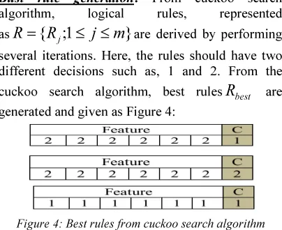
or a specific dissimilar constant.

Bust rule generation: From cuckoo search

algorithm, logical rules, represented

as

R

=

{

R

_j

;

1

≤

j

≤

m

}

are derived by performing

several iterations. Here, the rules should have two different decisions such as, 1 and 2. From the

cuckoo search algorithm, best rules

R

_best are

generated and given as Figure 4:

Figure 4: Best rules from cuckoo search algorithm

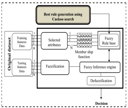
3.4.2 Classification using Neuro-Fuzzy:

Generation of fuzzy score using fuzzy system:

[image:7.595.92.288.572.689.2]

fuzzy interference system performs three dynamic functions as listed below:

• Fuzzification

• Rule Evaluation

• Defuzzification

[image:8.595.87.292.306.479.2]

Fuzzy inference is the unique procedure of generating a mapping from a prearranged input to the resultant output by the employment of a fuzzy logic. Thereafter, the mapping heralds a foundation and from this foundation appropriate decisions can be taken, and the patterns can be distinguished. The key task of fuzzy inference involves Membership Functions, Logical Operations, and If-Then Rules. The schematic graph of the fuzzy inference system (FIS) is vividly illustrated in Figure 5.

Figure 5: Fuzzy Inference System Structure

• Fuzzification

In fuzzification process, the crusty quantities are changed into fuzzy. In our proposed method, the fuzzification process is carried out by employing the features that are extracted in section 4.2.3. The

extracted features

are

F

T

F

NT

F

T

F

NT

F

T

and

F

NT

3 3

2 2 1

1

,

,

,

,

, for each

feature we perform fuzzification process. For the

fuzzification process, we collect all the

NT T

NT T NT T

F

and

F

F

F

F

F

3 3

2 2 1

1

,

,

,

,

features of the

training images and compute each feature minimum

(min) and maximum (max) values. The

fuzzification process is performed by the following equations.













−

+

=

3

min

max

min

]

[

₁T MinLimit

FL

(25)













−

+

=

3

min

max

]

[

FL

₁T MaxLimit

Max

Limt

(26)

In the above equations

[

FL

T₁

]

MinLimit and

Limit Max T

FL

]

[

₁ are the minimum and maximum

limit values of the feature

_F

₁T. The same equations

are used for the features

NT T

NT T NT T

F

and

F

F

F

F

F

3 3

2 2 1

1

,

,

,

,

to compute

the minimum and maximum limit values.

• Fuzzy Membership function:

The membership function of each and every input is recognized in this stage. The membership function is planned by selecting the appropriate membership function. One of the prominent challenges in all fuzzy sets involves the appropriate decision of fuzzy membership functions,

1) The membership function discharges its task

efficiently by performing the complete

demarcation of the fuzzy set.

2) A membership function furnishes an assessment

tool for estimating the level of resemblance of an element to a fuzzy set.

3) Membership functions may assume any shape;

however there occur certain general patterns which tend to emerge in bona fide applications.

• Rule Evaluation

Using cuckoo search algorithm, we already

generated the fuzzy rule set

}

,

1

;

{

R

j

m

T

R

_best

=

jbest

≤

≤

−

that are given in

the fuzzy rule base. The rule base contains a set of fuzzy rules.

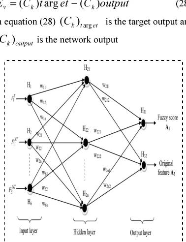
Neural network process: After the fuzzy

interference process, the fuzzy score is generated and assigned to the neural network output parameter. Totally, we have assigned two output classes (parameter), (i) fuzzy score (ii) original feature set. The neural network is well trained with these extracted features and different numbers of

unknown CT images are tested.The important steps

involved in neural network are shown in Figure 6, as follows,

Step 1: Put the input weights to every neuron except the neurons in the input layer. Here,

NT T

NT T NT T

F

and

F

F

F

F

F

3 3

2 2 1

1

,

,

,

,

are the input

of the network and

(

C

_k

)

output

is the decision result from the FIS and original feature set, i.e. output of the network.

Step 2: The neural network is designed with six

input layers,

_H

_ihidden layer, and two output layer.

The weights and then added to the neural network and it is biased.

Step 3: To the output layer the output of the activation function

f

(ln(

H

_i

))

is then broadcast all of the neurons:

)

(

)

(

1

2

C

n

W

output

C

l

N

n nl k

l

∑

=

+

=

η

(27)

Where

η

_i and

η

_k are the biases in the hidden layer and the output layer.

Step 4: Compute the error between the desired

output

C

_{k T et}

arg

)

(

and the output

₍

C

_k

₎

_output

produced by the feed-forward neural network, this is given by

output

C

et

t

C

E

_v

₌

(

_k

)

arg

₋

(

_k

)

(28)

In equation (28)

C

_{k t et}

arg

)

(

is the target output and

output k

C

₎

[image:9.595.94.283.410.656.2]

(

is the network output

Figure 6: Proposed neural network structure

In testing phase, the input testing feature

test

F

F

F

,

,

]

[

_{1 2 3} is given to fuzzy interference

system and corresponding fuzzy score is generated. This fuzzy score is given to the neural network. The resultant value of neural network’s output class is

represented as

A

₁and

A

₂, and this value is

compared with threshold value

T

₁.







≤

≥

=

1 2

1 1

;

;

Re

T

A

Normal

T

A

Abnormal

sult

₍₂₉₎

In this way the CT images are classified as normal and abnormal.

4. IMPLEMENTATION METHODOLOGY

This section presents the details about the simulation environment and the evaluation metrics are being discussed. The proposed approach of image denoising is experimented with the CT medical images and the result is evaluated with the PSNR and SDME. The obtained denoised image is then evaluated for the parameters sensitivity, specificity and accuracy for estimating the correctness of the image.

4.1 Simulation Environment

The proposed method is implemented in a Windows machine having a configuration of Intel (R) core I5 processor, 3.20 Ghz, 4 GB RAM and the operation system platform Is Microsoft Windows7 Professional. We have used Matlab latest version (7.12) for this proposed technique.

4.2 Evaluation Metrics

The formulae used to compute the evaluation metrics PSNR, SDME, sensitivity, specificity and accuracy values are given as follows.

4.2.1 Peak Signal to Noise Ratio (PSNR)

The formula for PSNR value computation is,

(

)

∑

−

×

×

=

_*

2 max 10

log

10

xy xy

h w

I

I

I

I

E

PSNR

Where, I_w and I_h Width and height of the

denoised image

Ixy Original image pixel value at

coordinate (x,y)

I*_xy Denoised image pixel value at

coordinate (x,y)

4.2.2 Second Derivative Measure of Enhancement (SDME)

The formula for SDME value computation [15] is, l k l k center l k l k l k center l k I I I I I I k k SDME , min; , , , max; , min; , , , max; 2 1 2 2 ln 20 1 + + + − − =

Where the denoised image is divided into (k_1×k₂₎

blocks with odd size,

I

max;_k,_l and

l k

I

min; , correspond to the maximum and minimum

values of pixels in each block whereas

_I

_center;_k,_lis

the value of the intensity of the pixel in the center of each block.

4.2.3 Sensitivity, Specificity and Accuracy

The evaluation of proposed technique in different CT images are carried out using the following metrics as suggested by below equations,

Sensitivity = negatives false of No positives true of No positives true of No . . . + Specificity = positives false of No negatives true of No negatives true of No . . . +

Accuracy = _{Nooftruepositives}Nooftrue_falsepositives_negativesnumber_trueof_negativestruenegatives_{falsepositives}

+ + + + . .

5. RESULTS AND DISCUSSION

In this paper, we have compared our proposed denoising technique against existing technique (Sachin D et al_{. [11]) with five CT images. The}

outcomes have shown that the performance of the proposed technique has significantly improved the PSNR and SDME compared with existing technique [11].

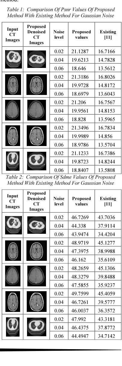
Table 1 shows the comparison values of Peak Signal to Noise Ratio (PSNR) for different noise variance levels for gaussian noise between the proposed method and the existing method.

Table 2 shows the comparison values of Second Derivative Measure of Enhancement (SDME) for different noise variance levels for gaussian noise between the proposed method and the existing method.

Table 3 shows the comparison values of Peak Signal to Noise Ratio (PSNR) for different noise variance levels for salt and pepper noise between the proposed method and the existing method.

[image:10.595.306.509.178.787.2]

Table 4 shows the comparison values of Second Derivative Measure of Enhancement (SDME) for different noise variance levels for salt and pepper noise between the proposed method and the existing method.

Table 1: Comparison Of Psnr Values Of Proposed Method With Existing Method For Gaussian Noise

Input CT Images Proposed Denoised CT Images Noise level Proposed values Existing [11]

0.02 21.1287 16.7166

0.04 19.6213 14.7828 0.06 18.646 13.5612 0.02 21.3186 16.8026 0.04 19.9728 14.8172 0.06 18.6979 13.6043

0.02 21.206 16.7567 0.04 19.9561 14.8153 0.06 18.828 13.5965 0.02 21.3496 16.7834 0.04 19.9989 14.856

[image:10.595.307.510.213.468.2]

0.06 18.9786 13.5704 0.02 21.1233 16.7386 0.04 19.8723 14.8244 0.06 18.8407 13.5808

Table 2: Comparison Of Sdme Values Of Proposed Method With Existing Method For Gaussian Noise

Input CT Images Proposed Denoised CT Images Noise level Proposed values Existing [11]

0.02 46.7269 43.7036 0.04 44.338 37.9114 0.06 43.9474 34.4204 0.02 48.9719 45.1277 0.04 47.3975 38.9988 0.06 46.162 35.6109

0.02 48.2659 45.1306 0.04 48.3279 39.8488 0.06 47.5855 35.9237 0.02 49.7599 45.4059 0.04 46.7261 39.5777

[image:11.595.91.290.154.401.2]

Table 3: Comparison Of Psnr Values Of Proposed

Method With Existing Method For Salt And Pepper Noise

Input CT Images

Proposed Denoised

CT Images

Noise level

Proposed values

Existing [11]

0.02 21.9445 21.634

0.04 21.0776 18.567 0.06 20.4357 17.0057 0.02 25.4193 21.8661 0.04 21.7599 18.918 0.06 20.5562 16.9189

0.02 22.5698 21.7306 0.04 21.2678 18.8978 0.06 20.5852 17.0635 0.02 22.1813 21.8897 0.04 21.4148 18.7489

[image:11.595.307.508.173.423.2]

0.06 20.8899 17.0178 0.02 21.7314 21.4638 0.04 21.1082 18.9884 0.06 19.9906 16.9854

Table 4: Comparison Of Sdme Values Of Proposed Method With Existing Method For Salt And Pepper Noise

Input CT Images

Proposed Denoised

CT Images

Noise level

Proposed Values

Existing [11]

0.02 69.9798 52.0768 0.04 64.9669 46.527 0.06 43.101 38.0931 0.02 67.5065 52.9996

0.04 65.2206 49.4154 0.06 44.0129 38.2141 0.02 67.9266 63.3859 0.04 64.7767 59.0446 0.06 43.7783 39.7519 0.02 64.3396 54.1842

0.04 68.8235 48.8421 0.06 43.8492 38.2939 0.02 65.8095 50.4402 0.04 63.1082 49.5018 0.06 42.0401 38.365

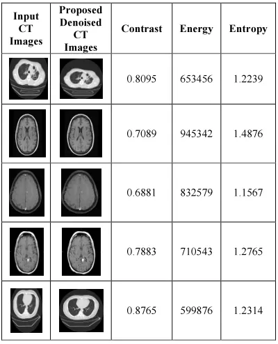
Table 5 shows the results after the extraction of features taking into consideration the parameters contrast, energy and entropy. The evaluation results

[image:11.595.308.508.175.422.2]

of the proposed against existing technique have shown better outcomes.

Table 5: Output Parameters After Feature Extraction

Input CT Images

Proposed Denoised

CT Images

Contrast Energy Entropy

0.8095 653456 1.2239

0.7089 945342 1.4876

0.6881 832579 1.1567

0.7883 710543 1.2765

0.8765 599876 1.2314

Sensitivity, Specificity and Accuracy graphs are shown in figure 7 to 9. In figure 7, the proposed approach achieved the sensitivity of about 96.3% whereas the existing approach achieved only 8.7% in training-testing ratio (70-30). In figure 8, the proposed technique achieved the specificity of 79.69% whereas the existing approach achieved only 72.27% in training-testing ratio (80-20). In figure 9, the proposed approach achieved the accuracy of about 79.89% whereas the existing approach achieved only 76.92% in training-testing ratio (90-10). Totally, the proposed tumour detection technique has obtained better performance evaluation when compared to the existing technique.

[image:11.595.94.291.441.689.2] [image:11.595.305.508.612.722.2]

[image:12.595.86.307.106.231.2]

Figure 8: Specificity graph of proposed with existing

Figure 9: Accuracy graph of proposed with existing

6. CONCLUSION

In this paper, we propose a new image denoising and classification technique using DTCWPT, EMD and CNF classifier. We have used two noises, Gaussian and salt & pepper for the proposed technique. The performance of the proposed image denoising technique is evaluated on the five CT images using the PSNR and SDME. For comparison analysis, our proposed denoising technique is compared with the existing work in various noise levels. The above calculations are being performed on an image of resolution 512×512 and work is being done to remove Gaussian and salt & pepper noise of the images and future plan is to make it valuable for different resolution and for different size of images. In the denoising phase Dual Tree Complex Wavelet Packets and Empirical Mode Decomposition are used for removing noise. In the segmentation process K-means clustering technique is employed. In classification, a modified technique called

Cuckoo-Neuro Fuzzy (CNF) algorithm is

developed and applied for detection of the tumour region. The cuckoo search algorithm is employed for training the neural network and the fuzzy rules are generated according to the weights of the training sets. Then, classification is done based on the fuzzy rules generated. From the obtained outcomes, we can conclude that the proposed denoising technique have shown better values for the SDME of 69.9798 and PSNR of 25.4193 for

salt & pepper noise which is very superior compared to existing methods. Moreover its performance was evaluated qualitatively and it has shown an accuracy of 96.3% which is much better when compared to existing methods.

REFERENCES:

[1] A.Velayudham, R.Kanthavel, “An Efficient Approach for Denoising of CT-Images Using EMD and Dual Tree Complex Wavelet Packets”, International Review on Computers and Software (IRECOS), Vol. 8 No. 9, pp 2088 – 2101, September 2013.

[2] O. Tischenko, C. Hoeschen, and E. Buhr, “An artifact-free structure saving noise reduction using the correlation between two images for

threshold determination in the wavelet

domain”, Medical Imaging 2005: Image Processing- Proceedings of the SPIE., J. M. Fitzpatrick and J. M. Reinhardt, Eds., vol. 5747, pp. 1066-1075, April 2005.

[3] Anja Borsdorf, Rainer Raupach, Thomas Flohr and Joachim Hornegger, “Wavelet based Noise Reduction in CT-Images using Correlation Analysis”, IEEE transactions on Medical Imaging, Vol. 27, No.12, 2008.

[4] N. Huang, Z. Shen, S. Long, M. Wu, H. Shih, Q. Zheng, N. Yen, C. Tung, H. Liu, “The empirical mode decomposition and Hilbert spectrum for nonlinear and non-stationary time series analysis”, Proceedings of the Royal Society of London, Vol. 454, pp: 903–995, 1998.

[5] G.Y. Chen,B.Kégl, “Image denoising with complex ridgelets”, Pattern Recognition, Vol. 40,pp.578-585, 2007.

[6] João M. Sanches, Jacinto C. Nascimento and Jorge S. Marques, “Medical Image Noise Reduction Using the Sylvester–Lyapunov Equation”, IEEE Transactions On Image Processing, Vol. 17, No. 9, September 2008. [7] Faten Ben Arfia, Mohamed Ben Messaoud,

Mohamed Abid, “A New Image denoising Technique Combining the Empirical Mode Decomposition with a Wavelet Transform Technique”, 17th International Conference on Systems, Signals and Image Processing, 2010. [8] Guangming Zhang,Zhiming Cui, Jianming Chen

and Jian Wu, "CT Image De-noising Model Based on Independent Component Analysis and Curvelet Transform”, Journal Of Software, Vol. 5, No. 9, September 2010.

[image:12.595.87.291.262.375.2]

Wavelet Transformation and Thresholding",

European Journal of Scientific

Research,Vol.48, No.2, pp.315-325, 2010. [10] G. Landi, E.Loli Piccolomini, "An efficient

method for nonnegatively constrained Total Variation-based denoising of medical images corrupted by Poisson noise," Computerized Medical Imaging and Graphics ,Vol.36, pp. 38- 46, 2012.

[11] Sachin D, Ruikar and Dharmpal D Doye, "Wavelet Based Image Denoising Technique", International Journal of Advanced Computer Science and Applications, Vol. 2, No. 3, pp. 49-53, 2011.

[12] Shanshan Wang, Yong Xia, Qiegen Liu, Jianhua Luo, Yuemin Zhu, David Dagan Feng, "Gabor feature based nonlocal means filter for textured image denoising", J. Vis. Commun. Image R., Vol.23, pp.1008-1018, 2012. [13] Ehsan Nadernejad, Mohsen Nikpour, "Image

denoising using new pixon representation based on fuzzy filtering and partial differential equations”, Digital Signal Process ing,Vol.22, pp.913-922, 2012.

[14] V Naga Prudhvi Raj, Dr T Venkateswarlu, "Denoising of medical images using dual tree

complex wavelet transform”, Procedia

Technology, Vol.4, pp.238-244, 2012.

[15] Karen Panetta, Yicong Zhou, Sos Agaian, and Hongwei Jia, "Nonlinear Unsharp Masking for

Mammogram Enhancement”, IEEE

Transactions On Information Technology In Biomedicine, Vol. 15, No. 6, November 2011. [16] Abdolhossein Fathi and Ahmad Reza

Naghsh-Nilchi, “Efficient Image Denoising Method Based on a New Adaptive Wavelet Packet Thresholding Function”, IEEE Transactions On Image Processing, Vol. 21, No. 9, September 2012.

[17] Sudipta Roy, Nidul Sinha, Asoke K. Sen, “A New Hybrid Image Denoising Method”,

International Journal of Information

Technology and Knowledge Management, Vol. 2, No. 2, pp. 491 - 497, December 2010. [18] Shutao Li, Leyuan Fang and Haitao Yin, “An

Efficient Dictionary Learning Algorithm and Its Application to 3-D Medical Image Denoising”, IEEE Transactions On Biomedical Engineering, Vol. 59, No. 2, February 2012. [19] Minakshi Sharma and Dr. Sourabh Mukharjee,

“Brain Tumour Segmentation using hybrid Genetic Algorithm and Artificial Neural Network Fuzzy Inference System (ANFIS),” International Journal of Fuzzy Logic Systems, vol.2, no.4, pp.(31-42), 2012.

[20] Jitendra malik, Serge belongie, Thomas leung and jianbo shi, “Contour and Texture Analysis for Image Segmentation,” International Journal of Computer Vision, vol.43, no.1, pp. 7-27, 2001.

[21] M. Rakesh, T. Rav, “Image Segmentation and Detection of Tumor Objects in MR Brain

Images Using Fuzzy C-Means (FCM)

Algorithm,” International Journal of

Engineering Research and Applications, vol.2, no.3, pp.2088-2094, 2012.

[22] Dr. H. B. Kekre and Ms. Saylee M. Gharge, “Image Segmentation using Extended Edge

Operator for Mammographic Images,”

International Journal on Computer Science and Engineering, vol.2, no.4, pp. (1086-1091), 2010.

[23] Jue Wu and Albert C.S Chung, “A novel framework for segmentation of deep brain structures based on Markov dependence tree”, NeuroImage, vol.46, pp. 1027-1036, 2009. [24] A.k.Qin and David A.Clausi, “Multivariate

Image Segmentation Using Semantic Region Growing with Adaptive Edge Penalty”, Image processing, IEEE Transaction, vol.19, no.8, pp.92157-2170), 2010.

[25] Tao Wang, I.Cheng and Basu, “Fluid Vector Flow and Applications in Brain Tumor Segmentation”, Biomedical Engineering IEEE Transactions, vol.56, no.3, pp. (781-789), 2009.

[26] Zafer Iscan, Zumray Dokur and Tamer olmez, “Tumor detection by using Zernike moments on segmented magnetic resonance brain images”, Expert Systems with Applications, vol.37, no.3, pp. (2540-2549), 2010.

[27] Reza Farjam,Hemant A.Parmar ,Douglas C.Noll ,Christina I.Tsien and Yue Cao,“ An approach for computer-aided detection of brain metastases in post-Gd T1-W MRI”, Magnetic Resonance Imaging, vol.30, no.6, pp. 824-836, 2012.

[28] A. K. Jain, “Data clustering: 50 years beyond K-means”, Pattern Recognition Letters, vol. 31, no. 8, pp. 651-666, 2010.

[29] R. Chitta and M. N. Murty, “Two-level K-means clustering algorithm for k-τ relationship establishment and linear-time classification”, Pattern Recognition, Vol. 43, no. 3, pp. 796-804, 2010.