Neural Pattern Similarity and Visual Perception

(1)

Neural pattern similarity and visual perception

Thesis by

Jonathan Harel

In Partial Fulfillment of the Requirements for the Degree of

Doctor of Philosophy

California Institute of Technology Pasadena, California

2012

(2)

(3)

(4)

Acknowledgments

Although my path at Caltech to the present moment has been circuitous, confusing, and difficult, along the way, I have had the privilege of being rewired and transformed by countless interactions with so many thoughtful people who challenged and impressed me. I would like to humbly offer here my deepest gratitude to my advisers, to whom I am forever indebted: Robert McEliece, for his unusual clarity of thought and crystalline explanations of information theory, for his seeing some potential in and offering me my first opportunity to research a problem (the practical workings of poset belief propagation), for inviting me to pursue a Ph.D. and generously continuing to support me even after I had decided on a change of direction; Pietro Perona, whose work in vision first interested me in the topic, and for our lengthy discussions deconstructing surprise and saliency; Christof Koch, who first interested me in neuroscience, for his enormous doctor-fatherly patience with me as I wended my way from visual attention to an interest in decoding brain activity, for his inspiring and invigorating full-throttle passion in the search for truth from all branches of human endeavor; Ralph Adolphs, whose talent in understanding, organizing, and managing of people is exemplary, for his generosity in guiding me through my last two years, and for his focused creativity and fruitful mentorship which contributed most significantly to originating and shaping the content of this thesis. I would also like to thank the chairman of my thesis committee, Jehoshua (Shuki) Bruck, for his time, effort, and support of my unconventional thesis topic for the department of Electrical Engineering.

(5)

taught me among many other things the importance of ridge regression, nonparametric hypothesis tests, and a patience with and reverence for the delicate, incremental findings born in the progression of experimental neuroscience.

Ronnie Bryan, a great and imaginative friend, directly contributed his code (keypoint annotation and face morphing), time, and ideas to the work in Part I, and Catherine Holcomb competently and diligently facilitated many, many hours of brain scans for me. Alex Huth deserves credit for introducing me to a beautiful experiment which would change my course towards neuroimaging1_{, for}

guiding me through my early encounters with its application, for helping me collect and retinotopize data for Chapter 4, and above all for expanding my social horizons and being an awesome friend. Cendri Hutcherson introduced me to SPM; Julien Dubois, Dan Kennedy, Jed Elison, and Mike Tyszka helped organize my thoughts about the results in Chapter 3 (Mike also has come to the rescue on many occasions with technical wizardry magnetic resonant); Melissa Saenz mentored me in my work with synesthetes, which became the basis for Chapter 5. I am thankful for these valuable contributions, without which this thesis would never have been possible.

I greatly enjoyed fraternizing with, and am most grateful for the encouragement I received from, Mortada Mehyar, Xiaodi Hou, Moran Cerf, and Kalen Jordan. These friendships have kept me sane and I will fondly remember all the foolish times together.

I would also like to thank the members of the Klab and the Adolphs Lab, and all the other quirky, clever, and adventurous people I’ve had the pleasure of meeting while at Caltech, including Sotiris Masmanidis, Himanshu Mishra, Uri Maoz, Rosemary Rohde, Costas Anastassiou, Amy Chou, Dirk Neumann, Alice Lin, Shuo Wang, Florian Mormann, Naotsugu Tsuchiya, Damian Stanley, Fatma Imamoglu, Kerry Fender, and Craig Countryman.

I wish to thank the subjects of my fMRI experiments, who bravely volunteered hours of their time to lie still in a dark, claustrophobic, and cacophonous tunnel, while I both annoyed and bored them with flashing images, in hopes of possibly understanding just a little bit more about what goes on in the brain during visual perception.

Finally, I wish to express my heartfelt gratitude to my family: to Anat and Kevin for all their love and warmth throughout the years, and for their intoxicatingjoie de vivre, and most importantly to my parents, whose scientific worldview set me on this trajectory long before I was able to appreciate it, and whose boundless love and endless support I am embarrassingly fortunate to have received.

(6)

Abstract

This thesis addresses the question of whether people actually see the same visual stimuli somehow diﬀerently, and under what conditions, if so. It is an experimental contribution to the basic un-derstanding of visual and especially face perception, and its neural correlates, with an emphasis on comparing patterns of neural activity driven by visual stimuli across trials and across individuals. We make extensive use of functional magnetic resonance imaging (fMRI); all inferences about neural activity are made via this intermediary. The thesis is organized into two parts:

In Part I, we investigate the nature of face familiarity and distinctiveness at perceptual and neural levels. We first address the question of how the faces of those people personally familiar to a viewer appear different than they would to an unfamiliar viewer. The main result is that they appear more distinctive, i.e., dissimilar to and distinguishable from other faces, and more so the higher the level of familiarity. Having established this connection between face familiarity and distinctiveness, we ask next what is different about the perception of such faces, as compared with indistinct and unfamiliar faces, at the level of brain activation. We find that familiar and distinctive faces are represented more consistently: compared with indistinct faces, which evoke slightly different patterns of activity with each new presentation, these faces evoke slightly similar patterns. Combined with the observation that consistency can enhance memory encoding (a result reported by Xue et al. [102]), this suggests a cyclic process for the learning of unfamiliar faces in which consistent representation and the presence of newly formed memories mutually feedback on each other.

(7)

related categories. We also show that one subject’s brain activity can be accurately modeled using another’s, and that this allows us to predict which image a subject is viewing based on his/her brain activity. Then, in a diﬀerent experiment investigating the perception of dynamic/video stimuli, we find evidence that when watching videos with sound, visual attention is likely blurred at times and transferred to audition; subjects relatively temporally decorrelate in visual areas compared to the muted case, in which the patterns of neural activity correlate across subjects at an average of 78% the level found with oneself later in time.

(8)

Introduction

Continually fluctuating streams of multicolored photons flow into the eye of an observer, lighting a grid of firing patterns among photoreceptive retinal neurons, sparking a chain reaction which spreads out into midbrain and through primary visual cortex, to higher reaches of the brain, where eventually a belief somehow emerges about the contents and configuration of the world. In between the cryptic and specific signals at the retina and the sweeping abstractions represented by individual neurons at high-level regions in the brain is a vast array of organized and back-feeding neural networks of increasingly general purpose. This thesis quantifies and compares the measurable activity of this process ofvision,across time and across individuals.

One motivation for implementing this particular research program was to come closer to un-derstanding how visual qualia, those internal experiences of conscious visual states, e.g., how the color red seems, compare across people. We can begin to provide some clues to the answer by quantitatively comparing visual cognition at its various levels, starting from its behavioral output and moving down to its cortical manifestations. To the extent that these subprocesses are similar across individuals, it is plausible that the accompanying qualia are too, as it seems unlikely that such similar physical processes could lead to very diﬀerent mental states; however, this relates to what David Chalmers calls the hard problem of consciousness [15], and philosophers may disagree on whether the question is ultimately tractable, especially in this way. But if we take the practicable view that qualia are defined by their physical or informatic relationships to other mental states, as in Tononi’s formalism [91], this style of investigation may prove fruitful.

(11)

MRI scanner with image projected

onto a screen in the back of the bore

MRI facility at Caltech

Subject-carrying table slides in

subject’s head goes here

Figure 1.1: Photographs of the human MR scanners at Caltech

humans and other animals. It is currently the best tool for achieving such whole-brain simultaneous coverage.

1.1 Neuroimaging with fMRI; visual cortex; faces

fMRI fMRI data are collected in MR scanners like the ones shown in Figure 1.1. An imaging subject enters the bore of the powerful and noisy superconducting magnet in the supine position for periods of 5 minutes to 1 hour at a time. During this time, bursts of radio-frequency energy are transmitted from a coiled antenna around the subject’s head at a frequency resonant with the precession of hydrogen nuclei inside the magnetic field. The energy in these bursts temporarily excites the hydrogen nuclei out of alignment with the main magnetic field, the aggregate eﬀect of which is magnetic flux through the transceiver head coil, inducing currents with characteristic relaxation time constants (such as T2*) which depend on the chemical environment (including relative concentration of deoxygenated hemoglobin) in which the hydrogen nuclei are embedded. Together with a systematic varying of the strength of the main magnetic field depending on the position in the scanner, and a frequency coding scheme, this endows the induced currents with information suﬃcient to reconstruct an image of the brain, one 2D slice at a time.

(12)

demands of the brain, it has nonetheless been repeatedly shown to significantly correlate with the actual activity of neurons, specifically their local field potentials, especially in the gamma range, and to a lesser extent with spiking activity (see, e.g., Logothetis [62], [61] for careful explanation). We will take this relationship between the fMRI signal and neural activity as an assumption when interpreting our results.

For our purposes, the useful data from an fMRI scan of one subject can be summarized as a matrix β where the rows index individual “voxels” (3D pixels), i.e. discrete points in the brain,

each of which may be assigned a regional label (such as “FFA” or “STS”), and the columns index either stimuli (Chapters 3 and 4) or equivalently time points for a single changing/dynamic stimulus (Chapter 5). Then βij = response to stimulusj at voxeli: a β or “beta” value is an estimate

of the hemodynamic response amplitude at a particular location (viz., a voxel) in the brain to a particular stimulus. For this reason, beta values will also be called response amplitudes, or response magnitudes. A column of thisβ matrix may be considered aspatial neural pattern, and a row may

be considered atemporal neural pattern (used only in Chapter 5).

Visual cortex For the work presented in this thesis, fMRI neuroimaging is mainly used to record

activity in visual cortex. Some of the distinct regions inside visual cortex can be organized into a hierarchy, like the one shown in Figure 1.2. This includes primary visual cortex (V1), where an individual neuron responds only to visual input from a very restricted part of the visual field, and specifically to simple features within this field such as a bar or grating oriented at a specific angle (see [45] for original work and [69] for a theoretical model of it). V2, V3, and V4 are outwardly spread from V1 on the cortical surface, and are associated with incrementally larger and more flexible receptive fields. In order to gain some intuition about the kinds of features represented by intermediate-level neurons, see Figure 1.3; Gallant et al. [28] found neurons in monkey V4 highly selective for such stimuli.

Faces are special We devote half of this thesis to just one category of visual stimulus, focusing

(13)

Figure 1.2: A schematic representation of the hierarchical processing stages through various regions in the primate visual cortex (adapted from [82]). The neurons in primary/low-level visual cortex (V1/V2) fire when simple visual features (such as oriented lines) occur in highly specific, small regions of the visual field (their receptive field sizes are small, 0.2₋1.1◦ _{of visual angle). These}

[image:13.612.110.543.56.411.2]

combine into progressively more generalized features until somewhere high in cortex (such as the prefrontal cortex), a specific label such as “animal” can be applied to the input.

Figure 1.3: Example stimuli (nonstandard gratings) used by Gallant et al. [27, 28] to characterize the tuning of neurons in macaque monkey visual area V4.

(14)

FACES

LEGEND NEURAL PATTERN

ACROSS SUBJECTS GENERAL VISUAL INPUT

static images from multiple categories

moving/dynamic images

WITHIN ONE SUBJECT

Chap 2

Chap 3

Chap 4

Chap 5 VISUAL STIMULUS INPUT

spatial pattern

temporal pattern

same stimulus, different trials

between different stimuli COMPARISON

familiar

distinctive

Figure 1.4: The visual stimuli and analyses used in each chapter are connected by logical arrows, meant to aid the reader to infer relationships such as “In Chapter 4, the spatially distributed neural patterns elicited by diﬀerent static images are compared within a subject, then these diﬀerences are compared across subjects.” or “In Chapter 2, a connection is established between familiar and distinctive faces.”

occipital, and frontal lobes (see [93, 94, 95, 65]). A very wide range of other brain areas have been found to be involved in the perception of faces as well [39, 31, 49, 55, 59, 60], including hippocampus and amygdala [26, 58], and even primary auditory cortex [43]. A stronger case could not be made for any other category of visual stimulus.

1.2 Organization of thesis

(15)

by using one element per time point then comparing the resultant temporal patterns in analogous brain locations.

1.2.1 Important brain regions mentioned throughout thesis

For reference, we provide a list of some important brain regions, their abbreviations, and associated functions:

� V1, primary visual cortex, also known as striate cortex [45, 18];

� V2, prestriate cortex, adjacent to and receiving feedforward connections from V1 [84];

� V3, third visual complex, a part of early visual cortex immediately adjacent to V2 [84];

� V4, part of extrastriate visual cortex, associated with intermediate visual features including

gratings [27, 28];

� MT, originally “medial temporal” (but not in humans), an area of visual cortex associated with the representation of visual motion [92];

� LO (orLOC), lateral occipital cortex/complex, associated with visual objects [35];

� Fusi, the fusiform gyrus, a ventral stream part of visual cortex associated with high level object representation including faces and words [63];

� FFA, the fusiform face area, an area in fusiform gyrus which is face-selective [50];

� STS, superior temporal sulcus, associated with many functions, including audio-visual

inte-gration [5];

� IT, inferior temporal cortex, associated with face processing and other high level vision [56];

� Cuneus, associated with basic visual processing and inhibition [36];

� Precuneus, associated with self-perception and memory [14];

� PostCing, posterior cingulate cortex, associated with many functions, including awareness,

memory retrieval, and familiarity [88];

� AntCing, anterior cingulate cortex, associated with motivation and attention [12];

(16)

Part I

(17)

Chapter 2

Personally familiar faces appear to be

more distinctive

Based on experiments involving ten human subjects, we conclude that faces which are familiar to a viewer appear to look more different from other faces than they do to unfamiliar viewers: that is, they appear more distinctive. Furthermore, we find evidence that faces which are entirely unfamiliar, merely similar in appearance to a familiar face, can be more easily distinguished than ones distant from any familiar face. These two effects taken together constitute a warping in the entire perceptual space around a learned face, pushing all faces in this region away from each other. We additionally show that the fact of familiarity with a face is predictable from performance level on a visual distinguishability task, and provide some preliminary results characterizing how facial features weigh differently when comparing familiar faces.

2.1 Previous work

(18)

Figure 2.1: An illustration of a 3-dimensional “face space” (adapted from Leopold [59]), including the origin, at which we find the most average looking face, and several faces along orthogonal directions. Caricatures are defined as faces extrapolated beyond their true position in this space to a position more distant from the origin but along the same direction: e.g., F2* is a caricature of F2, and F3* is a caricature of F3.

patterns of single neurons in the anterior infero-temporal cortex of macaque monkeys, supporting the norm-based view.

Several authors have written on the relationship between familiarity and distinctiveness. Valen-tine and Bruce [97] wrote, in the context of an earlier hypothesis: "If judgements of distinctiveness depend upon some mean of a large population of faces, familiarity with a particular face should not alter its perceived distinctiveness.” However, in their study, familiarity and distinctiveness were rated by two mutually exclusive sets of subjects respectively, so any reported relationship would bear on only memorability as an intrinsic property of a face, not on actual familiarity: they go on to provide data showing a positive but insignificant correlation between this independently rated familiarity of a face and its distinctiveness. Vokey and Read [99] found that familiarity and dis-tinctiveness were anti-correlated; however, in their study familiarity was actuallyentirely imagined

(subjects were misled to believe that some face stimuli were of people at the same school).

(19)

familiar face created a greater orientation after-eﬀect than an unfamiliar face. As we shall see, these last two studies are compatible with the findings reported in this chapter, insofar as familiar faces are associated with a kind of heightened perceptual acuity.

Under a strictly norm-based model of face coding, one would expect little or no systematic relationship between the distinctiveness of a face and its degree of familiarity. Perhaps as a face is in the process of being learned, its position in face space would slowly converge on a final position from an initially noisy estimate, but, on average, one would not expect it to end up systematically more nor less distant from the origin, that is, different in distinctiveness, than it started. Also, its contribution to shifting the global experiential average, and thus its effect on the perception of other faces, would be very minor or negligible. However, under the exemplar-based coding model, after a face is learned, it can be used to help resolve subtle differences between faces which were previously distant from any reference, by adding a new one inside a neighborhood of comparability.

The results in this chapter show what happens to the perceptual face space around a familiar face.

2.2 Basic experimental setup

70 75 80 85 90 95 100

1 2 3

Percent Correct (Bin)

Number of Subjects

Cambridge Face Memory Test Subject Performance Distribution

Figure 2.2: All ten participants scored in the normal range (score > 60) of face-recognition ability, as assessed by the Cambridge Face Memory Test ([23], http://www.faceblind.org/facetests/). Note, however, that one subject’s (S0’s) performance is a bit unusually low relative to the others.

(20)

them using keyboard inputs, explicitly and implicitly (see below). The subjects were all Caucasian females, a selection intended to eliminate gender and race eﬀects, which are known to influence face perception and which have already been extensively studied [13, 32, 68, 96, 3].

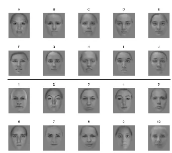
[image:20.612.147.489.166.471.2]

2.2.1 Participants

Figure 2.3: Each subject (A, B, ... J) is shown in the top half, with her sister occurring somewhere in the bottom half (1, 2, ... 10). Can you guess the 1:1 mapping between subjects and sisters? The answer key is given in Figure 2.48.

(21)

Whole Face

Inner Face

Figure 2.4: An example face from the dataset masked to include hair and jawline (left), and to only reveal inner features (right). The SimRate task was performed with both kinds of masks, but MorphDiscrim was performed only with inner faces.

2.2.2 Face stimuli

The face stimulus set consisted of forty “base” faces (the word “base” is used to distinguish these faces from “morph” faces, blended from these base faces and used in a later experiment described in Chapter 3). The faces were all emotionally neutral, front-facing, directly-gazing, Caucasian females organized as follows:

� 10 of the images were of the subjects themselves,

� 10 were of their sisters (one full biological sister per subject, age range 23 - 29, mean 26.3±

0.67 years), and

� 20 “extra stimuli”: eighteen were photographed in controlled conditions at Caltech1_{, and two}

were selected from the PUT Face Database [51].

All women in the stimulus set appeared to be in their twenties or early thirties at the time of their photograph. The pictures of the subjects’ sisters were obtained after sending them written instructions aimed at matching the conditions of the rest of the photographs (head-leveled camera, 5-6 feet away). Figure 2.5 shows all forty base faces used in the experiment, using a preparation hiding jaw and hairline, that is, including only inner face features (referred to later as “inner only”), Figure 2.3 shows the 10 subjects and 10 sisters stimuli2 _{in a preparation including jaw and hairline}

(“whole face”), and Figure 2.4 shows one stimulus in both preparations side-by-side. Importantly, 83 keypoints (e.g. left eye lateral extremity, or nose tip) were manually annotated on each face.

1_{thanks to Jan Glaescher for contributing some of these}

(22)

Figure 2.5: The forty base face stimuli, resized for equal proportions, and normalized for mean and standard deviation in luminance. Normalization beyond this (e.g., local contrast) was not carried out in order to allow some variability in low-level features. Subjects only viewed one face at a time at full scale (~355 pixels tall); faces are only combined here into a single image for spatial compactness.

Together with the pixel content of an image, this allowed us to compute objective distances between faces based on image content alone. See section 2.10.2 for additional details on stimulus preparation.

2.2.3 In this thesis, familiarity = personal familiarity

In this chapter and the next, we will refer to faces as familiar to a viewer, or reciprocally, a viewer as familiar with a face. Without exception, familiarity will herein mean, personal familiarity: the viewer will have had personal acquaintance with and knowledge of the person whose face they are said to be familiar with. All stimuli in the experiments are ultimately familiar in the less strict sense of having ever seen before in any context. The nature of the experiments was such that viewers saw all the faces many times by the end. The number of experimental trials during which a subject saw a face was not at all factored into level of familiarity at any point in the analysis.

Measuring degree of familiarity Because eight of the ten subjects and eighteen of the twenty

(23)

for 25th, 50th, and 75th percentiles of number of familiar faces among subjects including self and sister). The degree or level of personal familiarity each subject had with each person represented in the stimulus set was acquired through an interview with the author. Personal familiarity was assigned a

� 10 for self,

� 9 for sister,

� 8 for friend seen very frequently (every day),

� 7 for friend seen slightly less frequently, and so on, down to

� 1 for possibly seen around campus, and

� 0 for do not recall having ever seen before.

0 1 2 3 4 5 6 7 8 9 10

1 2 3 4 5 6 7 8 9 10

Familiarity Level

Number of Face Stimuli

Distribution of familiarity levels among subjects and stimuli

346 ..

Figure 2.6: Number of face stimuli, summed across subjects, at each level of familiarity. There are 54 total having level≥1, 45 having level > 1, and 36 total having level≥7.

In this chapter, unless otherwise specified, “familiar” as a category will mean familiarity > 1, and unfamiliar will mean familiarity ≤ 1 (i.e., the “possibly seen around campus” condition was

considered too weak to count as familiar).

2.2.4 Experimental Tasks

Two experimental tasks were employed, each measuring the visual similarity between face pairs as perceived by the subjects; we herein call these tasks “SimRate”, for Similarity Rating, and

(24)

InSimRate, the similarity between faces wasexplicitlyprovided by subjects using a numerical score from 1 (least) to 8 (most similar). InMorphDiscrim, the similarity between a pair of faces

was implicitly provided in the form of a confusability rate, measuring how frequently subjects

confused two distinct morphs (between a pair of faces) for two presentations of an identical face: the task was to tell whether a pair of morph stimuli were the same or different, when in half the trials they were actually the same. The rationale for this was that the more different the two base faces (from which the morphs were generated) appeared to look to the viewer, the easier a same/different discrimination between intermediate morphs would be to the subject, leading to a lower confusability rate.

In both experiments SimRate and MorphDiscrim, face pairs were never viewed simultaneously; instead, a base face or face morph centered on the screen was flashed for a brief interval (200 ms or less), followed by another face stimulus after a brief intervening visual “mask” to clear the space in between, followed by an interval during which the subject keyed in a response. See Section 2.10.4 for exact details about the trial structure used in these experiments.

Similarity scores across face pairs were Z-scored for each subject independently (that is, normal-ized to have sample mean 0 and sample standard deviation 1; see Section 2.10.1.1), and confusability scores were inferred from error rates in morph discrimination (see Eq. 2.2 for details). Among all subjects and face pairs, the similarity scores ranged from a minimum of -2.10 to a maximum 2.51. The minimum confusability score among all subjects and all face pairs was 0, and the maximum was 1.33. Distinguishability was defined as negative confusability (i.e., ranging from a minimum of -1.33 to a maximum 0).

(25)

2.2.5 RSMs and RDMs

The result of the SimRate and MorphDiscrim tasks can be completely summarized in what we will refer to as representational similarity matrix, RSM, or representational dissimilarity matrix, RDM (one for each subject, for each task). In the case of MorphDiscrim, the values are confusability for an RSM and distinguishability for an RDM. We will use these two somewhat interchangeably in some contexts as the only diﬀerence between them is that one is the negative of the other. The RSM is a symmetric matrixM whose entryMij is the similarity (or confusability) measure between stimulus

iand stimulusj.

0 0.1 0.2 0.3 0.4 0.5 0.6 0.7 0.8 0.9 1

Percent Trials Indicated Identical

Raw Performance on Morph Discrimination

0 1 2 3 4 5 6

7 8

9

identical mid ± 10% mid ± 20%

Morph Face Pair Type unique subject (avg. across face pairs)

0 0.1 0.2 0.3 0.4 0.5 0.6 0.7 0.8 0.9 1 Confusability Normalized Performance 0 1 2 3 4 5 6 7 8 9

identical mid ± 10% mid ± 20%

[image:25.612.116.538.245.460.2]

Morph Face Pair Type unique subject (avg. across face pairs)

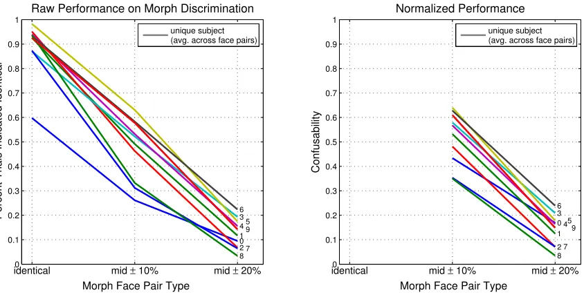
Figure 2.7: Each subject’s raw performance on MorphDiscrim is shown as an single line (subject number indicated at terminus), computed as the average over face pairs. Left: Each individual subject’s performance in the morph discrimination task is shown for the three levels used: (1) identical (faces actually the same), (2) mid ±10%, wherein each face was 10% removed from the

midpoint between the pair (in opposite directions), and (3) mid ± 20%, wherein each face in the

pair was 20% removed from the midpoint. Note that subject S0 appears to be an outlier in “identical condition”; she is also the outlier in Cambridge Memory – see Figure 2.32 for another comparison of Cambridge Memory score and experimental task performance. Right: A confusability metric is derived by dividing by fraction of trials indicated identical under the actually identical condition.

2.3 Raw performance results

(26)

Figure 2.7 confirms that subjects can more easily distinguish between faces on a morphing con-tinuum which are further apart. When the face morph stimuli are very similar (only 20% separated,

± 10% from the midpoint between a base pair), subjects perform at roughly chance level on

av-erage, indicating in about half the trials in which the faces are presented that they believe them to be identical. In the right panel of the same figure, we introduce aconfusability metric, which we define as the percentage of trials indicated identical when the faces are diﬀerent, divided by the percentage indicated identical when they actually are (see Eq. 2.2). This is computed separately for each face. We note here that when we refer to distinguishability or confusability, we will be referring to performance in the MorphDiscrim task, and when we refer to dissimilarity or similarity, we will be referring to performance in the SimRate task.

−1 −0.5 0 0.5 1 1.5

0 0.1 0.2 0.3 0.4 0.5 0.6 0.7 0.8

Subj Avg Morph Confusability

Subj Avg Reported Similarity

Reported Similarity vs. Confusability corr = 0.608

unique face pair

−0.6 −0.4 −0.2 0 0.2 0.4 0.6 0.8

0 1 2 3 4 5 6 7 8 9 10 11

Correlation (Indiv Var in Similarity v. Indiv Var in Confusability) (for single pairs rated > 0, excluding subj−sis pairs)

# face pairs

Individual Variability in Reported Similarity Corr’s with Individual Variability in Confusability

mean = 0.124, p

[image:26.612.111.531.280.510.2]

ttest=0.002 (n=53)

Figure 2.8: Subjects are consistent across the two types of face pair similarity tasks. Left: rela-tionship between subject-averaged similarity and confusability. Right: each point in the left panel corresponds to an average of 10 x- and y-coordinates, one per subject; each may be assigned a single-face-pair correlation between (i) subject variability in SimRate and (ii) subject variability in MorphDiscrim; the population of such correlations is shown for face pairs rated more similar than average (similarity in SimRate > 0) – it is significantly to the right of 0 by 1-sided t-test.

The left panel of Figure 2.8 shows that the subject-averaged similarity for a face pair in the SimRate task was correlated with the subject-averaged morph confusability, across the 118 face pairs for which both were measured, at a level of .608, with significancep <1.9×10−11_{, computed}

(27)

used extensively in this chapter and in this thesis; their p-values will often be denotedpshuﬀ. The

general method is described in Section 2.10.1.3. Figure 2.9 shows the correlation between subject-averaged dissimilarity and subject-subject-averaged confusability across face pairs, and compares this with distances based on low-level stimulus features.

Figure 2.9: The relationship between diﬀerent measures of inter-stimulus distance (first subject-averaged). We show the correlation between each such measure across face stimuli pairs. Distin-guishability and dissimilarity are most correlated (0.608), whereas pixel-based distance and keypoint-based distance are least (0.079). See Section 2.10.6 for methodological details and Section 2.9.4 for a comparison of distinctiveness measures.

(28)

left out of this analysis (right panel of Figure 2.8) the 10 pairs of subject-and-sister faces, due to an “insider information” eﬀect we shall discuss later (in Section 2.4.2.1). If subject-sister pairs are included in the right panel of Figure 2.8, the mean inter-individual correlation drops from 0.124 to .096, and the 1-sided t-test drops fromp <0.002 top <0.01.

2.4 Familiar faces are more distinct

−0.8 −0.7 −0.6 −0.5 −0.4 −0.3 −0.2 −0.1 0 0.1 0.2 −0.8 −0.7 −0.6 −0.5 −0.4 −0.3 −0.2 −0.1 0 0.1 0.2 S0 S1 S2 S3 S4 S5 S6 S7 S8S9

Face pairs are more distinguishable to familiar viewers ∆Dist

24 samples= 0.266 (pshuff = 7.4e−06, pbino = 1.8e−05)

Morph Distinguishability to Familiar Viewer (Fam

−

Fam)

Avg. Morph Distinguishability to Unfamiliar Viewers (UnFam−UnFam) (over other viewers)

7 other viewers

6

5

4

Unique Viewer, Fam. Stimulus Pair

Figure 2.10: A pair of faces, both familiar to a viewer, is more easily distinguished in MorphDiscrim than it is by viewers unfamiliar with either face in the pair (i.e., data falls above y=x line on average). The sizes of the circles correspond to the number of unfamiliar viewers averaged together for the x-coordinate (this number varies due to the familiarity structure between subjects and stimuli). The red colored circles correspond to the (self,sister) pairs of familiar faces, and are labeled with the corresponding subject number. The mean displacement above the diagonal across data point is 0.266 and is reported in the title.

(29)

2.4.1 Eﬀect on Morph Distinguishability

Figure 2.10 is the first in a series illustrating the enhanced distinctiveness of familiar faces. We see that pairs of faces, when they are both familiar to a viewer, are distinguished much more easily than when neither one of the faces if familiar to a viewer: the data lie above the y=x diagonal. In the same figure, we see that for all but subject S7, the pair of (self face, sister face) can be more easily distinguished by the subject viewing herself than by subjects unfamiliar with either.

Understanding the statistical significance values: The magnitude of the overall eﬀect is

highly significant, with an empirical significance ofpshuf f <7.4×10−6(again, see Section 2.10.1.3);

the null distribution is generated by randomly shuffling the occupied entries of the RDM while holding familiarity relationships constant. We tally the number of shuffled trials where at least as great an effect magnitude (in this case∆Dist24samples= 0.266) is observed, establishing an empirical

significance measure. For such plots, we also report a “binomial” significance value,pbino, which is

the probability of observing at least as many data points with y-coordinate>x-coordinate (in this case, distinguishability-to-familiar-viewer > distinguishability-to-unfamiliar-viewer) as we actually do, assuming the probability of each such event were 50%.

−0.8 −0.6 −0.4 −0.2 0 0.2

Face pairs are more distinguishable to half−familiar viewers

∆Dist

45 samples= 0.125 (pshuff = 2.9e−06, pbino = 2.7e−07)

Avg. Morph Distinguishability to Familiar Viewer (Fam

−

UnFam)

(over second faces)

Avg. Morph Distinguishability to Unfamiliar Viewers (UnFam−UnFam) (over second faces and other viewers)

50 second faces & viewers

35

20

5

[image:29.612.197.455.406.629.2]

Unique Viewer, Familiar Stimulus

(30)

We next investigate whether pairs of faces can be more easily distinguished even when only one face in the pair is familiar to the viewer; this is what we will refer to as a half-familiar viewer (or viewer only half-familiar with the pair). Figure 2.11 shows that such face pairs are indeed more easily distinguished, though the boost in distinguishability falls from 0.266 in the case of fully familiar pairs to 0.125 in the case of half familiar pairs. However, the eﬀect is highly significant under both empirical (pshuf f<2.9×10−6) and binomial tests (pbino<2.7×10−7).

−1.5 −1 −0.5 0 0.5 1 1.5

Face pairs are more dissimilar to familiar viewers ∆Dissim

67 samples= 0.294 (pshuff = 0.002, pbino = 0.0015) (Whole Face − Among all qualifying pairs)

Dissimilarity to Familiar Viewer (Fam

−

Fam)

Avg. Dissimilarity to Unfamiliar Viewers (UnFam−UnFam) (over other viewers)

8 other viewers

6

4

Unique Viewer, Fam. Stimulus Pair

Figure 2.12: A pair of faces, both familiar to a viewer, is rated more dissimilar than by viewers unfamiliar with either face in the pair. The sizes of the circles correspond to the number of unfamiliar viewers averaged together for the x-coordinate. (self,sister) pairs are excluded from this analysis due to “insider information” bias.

2.4.2 Eﬀect on Explicit Similarity Judgment

(31)

2.4.2.1 Insider information: influenced by the expectation of familial similarity

−0.50 0 0.5 1 1.5 2 2.5

1 2 3 4

self−reported sibling similarity −

avg. reported sibiling similarity among unfam. viewers

number of subjects (inside bin)

Self−reported facial similarity to sibling is too high (p<0.029)

Figure 2.13: “Insider information” The similarity between a subject’s own face and her sister’s is rated higher (to the right of 0 in the plot) than it is by entirely unfamiliar viewers likely due to knowledge of the familial relationship not known to the unfamiliar viewers. This eﬀect is significant by two-sided t-test (p <0.029).

(32)

2.4.2.2 Half-familiar face pairs are rated as more dissimilar

Next, we see in Figure 2.14 that, just as with the distinguishability of faces, their explicitly rated dissimilarity to others is greater even when only one of the two faces being compared is familiar to the viewer; that is, the half-familiar viewer perceives a pair of faces to be more diﬀerent looking than an entirely unfamiliar viewer. The average dissimilarity boost is smaller, at only 0.146, than was obtained for pairs of faces both familiar (0.294), but is highly significant: the probability of observing so many (viewer, familiar stimulus) combinations with trend going in the same bias direction is

pbino< 0.00019. We note that for this analysis, face pairs with dissimilarity > -0.25 (as rated by

others) are excluded. As we shall discuss later in Section 2.5.2, this is because fair pairs which are already very dissimilar looking do not becomeeven more dissimilar looking once when of them is familiar. However, this qualification is not necessary for the boost to be significant when considering ratings between inner faces only. See the Supplementary Figure 2.37 for this.

−1 −0.5 0 0.5 1

Face pairs are more dissimilar to half−familiar viewers

∆Dissim

44 samples= 0.146 (pshuff = 0.00028, pbino = 0.00019)

(Whole Face − Among more similar face pairs)

Avg. Dissimilarity to Familiar Viewer (Fam

−

UnFam)

(over second faces)

Avg. Dissimilarity to Unfamiliar Viewers (UnFam−UnFam) (over second faces and other viewers)

125 second faces & viewers

75

25

10

Unique Viewer, Familiar Stimulus

(33)

2.4.3 Eﬀect on neighborhood of familiar faces

familiar face

d₁ d2 d₃

Familiarity-induced expansions in face space

unfam. face

“fam neighborhood”-type expansion “fam-unfam”-type expansion

Figure 2.15: Illustration of changes in face space due to familiarity with a face stimulus. The unfamiliar faces are assumed to be in the neighborhood of faces which look similar to the familiar one, which we refer to as the “familiar anchor” of this region of face space, below.

We were interested in whether the expansion in face space around a familiar face (the perceptual distancing, in dissimilarity judgment and distinguishability) extends measurably beyond comparisons directly involving a familiar face. Figure 2.15 illustrates a second kind of change in face space we might expect: that between two unfamiliar faces merely close to a familiar face (termed a “fam

neighborhood” expansion and denoted with red arrows). The problem with assessing this kind of

eﬀect is establishing a perfect control subject, or contrasting case, because, based on the experimental limitations, we could not know whether two faces were actually in the neighborhood of a face familiar to a viewer, but one which was not in our stimulus set. Nonetheless, we could at least guarantee that the control subject not have a familiar face, from our stimulus set, close to the candidate pair of faces. We refer to this as theimperfect control condition. Below, we will refer to a viewer of a face pair, who is unfamiliar with both faces in the pair, but familiar with a face close to the pair (by some metric), as aquasi-familiar viewer.

(34)

−2 −1.5 −1 −0.5 0 0.5 1 1.5 −2 −1.5 −1 −0.5 0 0.5 1 1.5 ∆Dissim

218 samples= 0.261 (pshuff = 0.02, pbino = 2.9e−05) (famil>=9, among 3 closest faces)

Dissimilarity to Viewer in Fam. Neighborhood

Avg. Dissimilarity to Entirely Unfam. Viewers (over other viewers)

Unique (viewer, pair of unfam. faces close to a familiar one)

−2 −1.5 −1 −0.5 0 0.5 1 1.5

−2 −1.5 −1 −0.5 0 0.5 1 1.5 ∆Dissim

264 samples= 0.21 (pshuff = 0.06, pbino = 8.2e−05) (famil>=8, among 3 closest faces)

−2 −1.5 −1 −0.5 0 0.5 1 1.5

−2 −1.5 −1 −0.5 0 0.5 1 1.5 ∆Dissim

475 samples= 0.159 (pshuff = 0.08, pbino = 0.00024) (famil>=7, among 4 closest faces)

(35)

the top 60% of similarity, averaged across the 8 remaining subjects (not non- or quasi-familiar being compared). The eﬀect is most robust in the neighborhood of self face or sister’s face (eﬀect size: 0.261), corresponding to familiarity≥9, presumably because people have an especially great level

of expertise in this familial territory of face space, perhaps having other similar looking relatives whose faces they learned. The eﬀect size smoothly falls oﬀ to 0.210 when we include close friends and to 0.159 when we loosen the quasi-familiarity level further.

−1 −0.8 −0.6 −0.4 −0.2 0 0.2

−1 −0.8 −0.6 −0.4 −0.2 0 0.2 ∆Dist

(famil>=8, among 40% most confusable face pairs)

Morph Distinguishability to Viewer in Fam. Neighborhood

Morph Distinguishability to Entirely Unfam. Viewer Unique (viewer, pair of unfam. faces close to a familiar one)

−1 −0.8 −0.6 −0.4 −0.2 0 0.2

−1 −0.8 −0.6 −0.4 −0.2 0 0.2 ∆Dist

(famil>=7, among 40% most confusable face pairs)

Morph Distinguishability to Viewer in Fam. Neighborhood

Morph Distinguishability to Entirely Unfam. Viewer Unique (viewer, pair of unfam. faces close to a familiar one)

Figure 2.17: Distinguishability is relatively enhanced in the neighborhood of a familiar face. Left: Faces pairs are selected for analysis if the are each close to a familiarity-level 8 or greater face, where close means among 40% most confusable faces. Right: Faces pairs are selected for analysis if the are each close to a familiarity-level 7 or greater face. Each data point corresponds to a unique selection of (contrasting viewer, pair of faces being compared), but multiple data points can be produced by the same quasi-familiar viewer’s distinguishability; points are colored by unique quasi-familiar viewer.

(36)

size and significance. However, we found that by holding the RDM constant and instead shuffling the mapping between subject and stimulus familiarity, the empirical significance values improved: those are the ones reported in Figure 2.17 (and Figure 2.16). This is likely because, compared to shuffling the RDM, shuffling the familiarity mapping more completely disrupts the structure of distinctiveness biases. For each pair of faces in the fam neighborhood, a non-quasi-familiar viewer (represented by the x-coordinate in Figure 2.17) was qualified exactly as with SimRate above, except the face pair was required to not be in the top 25%, instead of 60%, of similarity in comparison with any face familiar to her (as rated by the other 8 subjects). The requirement was loosened in order to admit enough data points for analysis.

0 0.05 0.1 0.15 0.2 0.25 0.3 0.35 0.4 0.45 0.5 Both − Fam Half − Fam Quasi − Fam

Face Pair Dissimilarity Boost

dissim. (fam)

−

dissim. (unfam)

face pair familiarity type

0 0.05 0.1 0.15 0.2 0.25 0.3 0.35 0.4 Both − Fam Half − Fam Quasi − Fam

Face Pair Distinguishability Boost

disting. (fam)

−

disting. (unfam)

face pair familiarity type

Figure 2.18: A summary of dissimilarity and distinguishability boosts for diﬀerent categories of fa-miliar (or quasi-fafa-miliar) face pairs. Standard error bars are computed over unique subject-stimulus combinations (e.g., “unique viewer, familiar stimulus”), as described in the preceding section. Impor-tant note: To make the comparisons across all three categories of face pairs meaningful, familiarity was defined in each case (including quasi-familiar) to mean level≥7. Note that is diﬀerent from the scatter plots shown in the preceding section, which also include faces with lower familiarity levels, for completeness.

2.5 Factors aﬀecting the enhanced distinctiveness of familiar

faces

2.5.1 Degree of familiarity and distinctiveness boost

(37)

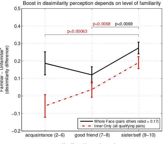
acquaintance (2−6) good friend (7−8) sister/self (9−10) −0.1

−0.05 0 0.05 0.1 0.15 0.2 0.25 0.3 0.35 0.4

p<0.00032 p<0.011

Familiar

−

Unfamiliar*

(distinguishability difference)

*familiar with exactly one face

Boost in distinguishability depends on level of familiarity

Figure 2.19: The degree of familiarity enhances distinguishability of faces (analysis is based on pairs of half-familiar pairs). p-values are based on 2-sided t-tests.

the boost in distinguishability when comparing with an unfamiliar face. We find that, on average, faces of oneself or one’s sister, or that of a good friend (familiarity 7 - 8), receive a larger boost in distinctiveness relative to less familiar faces. The result is shown in Figure 2.19, which is essentially the average displacement above the diagonal in Figure 2.11 by familiarity type, except leaving unique second viewers as unique data points for more statistical power. We note that we left out face pairs which had confusability score of less than 0.2 (33rd percentile), rated by the other 8 viewers, because, as we shall discuss shortly, face pairs which are already easily distinguished do not gain much in distinguishability from familiarity with one of them.

(38)

acquaintance (2−6) good friend (7−8) sister/self (9−10) −0.2

−0.1 0 0.1 0.2 0.3 0.4 0.5

p<0.00063

p<0.0069 p<0.0068

Familiar

−

Unfamiliar*

(dissimilarity difference)

Boost in dissimilarity perception depends on level of familiarity

[image:38.612.192.456.77.310.2]

Whole Face (pairs others rated > 0.17) Inner Only (all qualifying pairs)

(39)

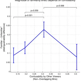
2.5.2 Baseline similarity/confusability and distinctiveness boost

0.15 0.2 0.25 0.3 0.35 0.4 0.45 0.5 0

0.05 0.1 0.15 0.2 0.25 0.3 0.35

p<0.021 p<0.059

p<0.068

Confusability by Other Viewers (Non−Overlapping Bins)

Familiar

−

Unfamiliar*

(distinguishability difference)

[image:39.612.191.460.112.381.2]

Magnitude of familiarity effect depends on confusability

Figure 2.21: The extent to which a face pair becomes more distinguishable to a familiar viewer depends on the underlying confusability of the pair.

(40)

face pair confusability, and so performance there floored, whereas face pairs near the middle of the confusability levels just admitted a broader performance range within which the familiarity eﬀect could be measured: this would suggest that perhaps the most similar looking face pairsactually are

most aﬀected by familiarity, both in terms of dissimilarity perception and distinguishability, but that the nature of our experimental setup prevented the accurate measuring of the latter. In either case, it is clear that the least confusable or similar face pairs are perceptually aﬀected least from familiarity.

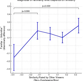
−0.4 −0.3 −0.2 −0.1 0 0.1 0.2 0.3

−0.3 −0.2 −0.1 0 0.1 0.2 0.3 0.4 0.5

p<0.088

p<0.039

Similarity Rated by Other Viewers (Non−Overlapping Bins)

Familiar

−

Unfamiliar*

(dissimilarity difference)

[image:40.612.191.460.225.490.2]

Magnitude of familiarity effect depends on similarity

Figure 2.22: The extent to which a face pair becomes more dissimilar to a familiar viewer depends on the underlying similarity of the pair.

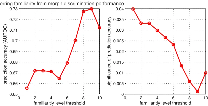
2.6 Predicting familiarity from distinguishability

(41)

0 2 4 6 8 10 0.65

0.66 0.67 0.68 0.69 0.7 0.71 0.72 0.73

prediction accuracy (AUROC)

familiaritiy level threshold

Inferring familiarity from morph discrimination performance

0 2 4 6 8 10

0 0.005 0.01 0.015 0.02 0.025 0.03 0.035 0.04

significance of prediction accuracy

[image:41.612.122.539.72.285.2]

familiaritiy level threshold

Figure 2.23: Based on the distinguishability of a pair of faces, it is possible to accurately predict, using a linear model, whether they are familiar at or above some threshold level. The familiarity of a pair is taken to be the maximum of the familiarity with either one of the faces in the pair.

Left: Average (across subjects) area-under ROC-curve showing the prediction performance level for each familiarity threshold,Right: statistical significance of each performance level determined using random shuﬄings of familiarity relationships.

the confusability by the test subject with possible familiarity:

M = [Cothers,meanCothers,minCself1], model: M w=F

whereCothers,mean is a column vector, one entry per face pair, containing the sample mean

confus-ability among subjects unfamiliar with the pair, Cothers,min is the minimum confusability among

these subjects, and Cself is the confusability as determined by the test subject. F is the column

vector of binarized familiarity. For each subject, we form a training data set by using data from all the remaining subjects, left out one at a time (leaving 8 possible others), as test subjects to form

Cself, and then find the optimalwwhich minimizes ||F−M w||via standard linear regression. We

then apply this learned w vector to the left-out subject’s ratings and assess the predictiveness of

M was an estimate ofF. The result is shown in Figure 2.23. The prediction performance associated

with the real-valued estimateM w of the binarized familiarityF was determined by an area-under

the ROC-curve (AUROC) analysis in which, for each thresholding ofM w, a true and false positive

(42)

to predict familiarity under a shuﬄed mapping of subject to stimulus familiarity. Higher levels of familiarity are easier to predict from distinguishability performance, but prediction accuracy peaks at separating self/sister (≥9) from all other types of familiarity (≤8). Separating the self face as

familiar from sister as unfamiliar, corresponding to threshold level 10, weakens prediction accuracy slightly. As one would intuitively expect, the average weight vectorweﬀectively subtracts the

con-fusability of the test viewer from that of unfamiliar viewers: the greater this diﬀerence, the more likely the subject is actually familiar: the entry inw corresponding to Cothers,mean is positive on

average (0.4), and the one corresponding toCself is negative (-0.8).

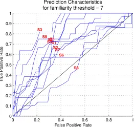
0 0.2 0.4 0.6 0.8 1

0 0.1 0.2 0.3 0.4 0.5 0.6 0.7 0.8 0.9 1

S0S1 S2 S3

S4S5

S6 S7

S8 S9

False Positive Rate

True Positive Rate

[image:42.612.194.458.243.493.2]

Prediction Characteristics for familiarity threshold = 7

Figure 2.24: ROC performance curves for predicting the familiarity (≥7) of each individual subject from distinguishability performance. Subject S8’s familiarity level is most diﬃcult to predict.

Predictability of familiarity from distinguishability and average familiarity eﬀect

size: There were some individual diﬀerences in the extent to which a subject exhibited a boost in

(43)

2.7 Factors contributing to face similarity perception

Although stimuli were relatively small (9◦_×₁₂◦ _{of visual angle) and briefly displayed (200 ms),}

thus discouraging both the need for and possibility of eye movements despite the experimental instructions to stay fixated at the center, naturally different subjects would occasionally move their eyes or covertly attend to different facial properties. In this section, we investigate how facial features, both holistic and localized, weigh differently in the perception of familiar faces relative to unfamiliar ones. We do this by modeling dissimilarity judgments between faces as driven by the inter-stimulus distances between single features, such as eye position or attractiveness. Refer to Section 2.10.5.2 for a detailed description of how a single feature is assigned a corrected significance level in modeling the dissimilarity judgments.

2.7.1 Independently-rated face properties and dissimilarity

An entirely separate set of 10 healthy adult subjects (7 male) participated in an online experiment,

FaceRate, in which each of the 40 face stimuli in our data set were rated for 18 holistic and localized features such as femininity, largeness of the eyes relative to average, and attractiveness. The face features were rated by subjects on a computer, in their own home, taking as much time as they wanted for each face, while being presented with the face stimulus (inner features only) on the screen, and a sliding-bar interface like the one shown in Figure 2.25.

Figure 2.25: A snapshot of part of sliding bar interface used by subjects in FaceRate. This was rendered in a browser and used by 10 participants to provide holistic and featural judgments about the 40 face stimuli.

(44)

[image:44.612.107.540.80.332.2]

Figure 2.26: Face dissimilarity judgments, between pairs of entirely unfamiliar faces, can be statistically significantly modeled using distances between single features. The significance values are written in the table and the color corresponds to −log10(p) . The values in the “All” row are

determined by modeling the subject-averaged dissimilarities.

metric for each of the face features. The rated face features are described in detail in Section 2.10.5.1, but they have mostly self-explanatory names.

Figures 2.26 and 2.27 show the result of modeling dissimilarity judgments in SimRate using the 18 face features provided by participants in FaceRate. Whereas in Figure 2.26 we model only those dissimilarity judgments between pairs of unfamiliar faces, in Figure 2.27 we model only the dissimilarity judgments between pairs in which at least one face is familiar. We see that for both kinds of comparisons, the size of the eyes relative to the face is an important: if one face has relatively smaller eyes, and the other relatively larger, this will on average be associated with a higher dissimilarity. This is likely in part explained by the fact that subjects were asked to fixate between the eyes.

The weights (−log10p)of features for the unfamiliar face pairs are on the whole positively

(45)

[image:45.612.109.539.79.332.2]

Figure 2.27: Face dissimilarity judgments, between half- or both-familiar face pairs, can be statistically significantly modeled using distances between single features. The significance values are written in the table and the color corresponds to −log10(p) . The values in the “All” row are

determined by modeling the subject-averaged dissimilarities (among those who are familiar).

qualitatively by examining the relatively higher scattering of brightness values on the right side of table showing weights for familiar comparisons. Also, whereas happiness does not significantly model unfamiliar comparisons (p <0.64), it does for familiar comparisons (p <0.0002). Although

the faces were all supposed to be emotionally neutral, inevitably subtle micro-expressions leaked through conveying some kind of nonzero emotional valence. The increased weighing of happiness in familiar comparisons is consistent with the hypothesis that we are more sensitive to detecting the emotional state of familiar faces.

2.7.2 Individual facial keypoints and dissimilarity

(46)

[image:46.612.110.540.117.588.2]

Figure 2.28: Face dissimilarity judgments, between pairs of entirely unfamiliar faces, can be statistically significantly modeled using distances between single features. The locations of keypoints which significantly model (viz., havingp_≤0.01) dissimilarity judgments betweenunfamiliar faces

are highlighted with a circular Gaussian kernel for illustration purposes. The standard deviation of this kernel (0.5◦of visual angle) was chosen to allow some fuzziness in the location of the underlying

(47)

[image:47.612.111.536.140.593.2]

Figure 2.29: Face dissimilarity judgments, between half- or both-familiar face pairs, can be statistically significantly modeled using distances between single features, shown highlighted where

(48)

For both comparisons involving familiar faces, and those which do not, we find individual facial keypoints which can statistically significantly model dissimilarity judgments. However, we find on average many more of these when modeling unfamiliar face comparisons. One possible simple reason might be that we have fewer data samples of dissimilarity judgments involving familiar pairs, so the average ratings are noisier and the individual ratings are sparse, making a significant fit more diﬃcult to achieve. However, this is unlikely because there were many examples of face features, rated in FaceRate and shown above, which significantly modeled only the familiar comparisons, not the unfamiliar ones, such as “nordicness” for subject S9, or “blemishedness” for subject S4, or happiness for several others. A more plausible explanation is that familiar faces are perceived and compared more holistically than unfamiliar faces, thereby eliminating a significant eﬀect of any one single keypoint location as our analysis here attempts to find for each individually. A related finding was reported by Heisz et al. [40], in which it was found that familiar faces (though not

personally familiar) under free viewing (3 seconds, compared to our≤0.2 seconds) were scanned by

eye movement less in some contexts (identity recall but not recognition of familiarity). If we suppose that eye movements are more diﬃcult to suppress or are otherwise more frequent for unfamiliar faces, this might mean that locally salient visual information plays a larger role in unfamiliar faces than for familiar faces.

The facial keypoint weightings in this subsection may be related to the independently-rated face features weightings, shown in the previous subsection; we list here several examples of consistency between the two: (1) subject S7 heavily weighs both nose-upturned-ness above, and nose keypoints here, in the case of familiar face pairs, (2) subject S6 weighs “archiness” (extent to which eyebrows are arched) heavily above, and eyebrow keypoints here, in the case of unfamiliar face pairs, (3) for subject S0, eye size is significant in unfamiliar face pairs above, but it is not for familiar ones, and the corresponding results are found with respect to eye keypoints here, (4) subject S8 heavily weighs face wideness above, and here keypoints along the side of the face which would cue face wideness, for unfamiliar face pairs, (5) the most significant rated feature above for subject S1 in the case of familiar face pairs is eyebrow archiness, and the only keypoint location we find significance for here is the tip of one of the eyebrows.

2.8 Discussion

(49)

entire neighborhood of faces around a familiar one. We summarize these eﬀects as a “distinctiveness boost” given to familiar faces. We also showed that it is possible to accurately predict whether a face is familiar based on a person’s ability to distinguish it from others. Lastly, we provided data suggesting that familiar faces are processed more holistically and with more attention to emotion.

We began the chapter with a discussion of norm-based coding vs exemplar-based coding in the brain. We discussed the implication that norm-based coding does not allow for familiar faces to look progressively more distinctive as they are learned. Now, it is easy to imagine how our results are consistent with the predictions ofexemplar-based codingof faces, wherein each new face is represented by its distances to familiar faces. If we assume that as a face is being learned its weighting in the distances-to-references representation increases, thus adding a new and stretching dimension to this face space, all faces would gradually push away from it, and from each other, leading to a perceptual expansion of the face space around it, consistent with the one we experimentally observe. That the eﬀect should be limited to only the neighborhood of a familiar face can be accounted for if we assume that reference faces beyond some threshold distance do not factor (e.g., one might not use an Asian male face reference to distinguish between two Caucasian females); analogously, in the brain, a neuron encoding a likeness to a reference face too dissimilar to the visual input may not fire at all, thus not contributing to its representation. However, although our results arenot compatible with strictly norm-based coding of faces in visual cortex, it is our view that visual cortex likely accommodates neurons implementing both norm-based and exemplar-based coding of faces.

It is easy to argue that the perception of familiar faces as more different looking confers an evolutionary advantage: for example, this would make it easier to pick out a familiar face in a crowd, thus facilitating more efficient acquisition of critical social information among competing or cooperating animals. The relative ease of visual search for such a stimulus was demonstrated in a classic paper by Duncan et al. [24], wherein it was shown that “[search] difficulty increases with increased similarity of targets to nontargets”. So a target face which is perceived to look dissimilar to nontargets would be found more easily. A related finding specific to faces was reported by Pilz et al. [71], who found that faces which were studied in motion, rather than as still images, were subsequently located more quickly in a visual search array.

Future directions: In defining familiarity, we did not account for number of stimulus

(50)

(51)

2.9 Supplementary results

(52)

2.9.1 There is consensus across subjects within tasks

0 0.2 0.4 0.6 0.8

Morph Confusability (by others)

Morph Confusability (by S0)

Subj S0 vs Others, Corr = 0.451

slope=0.801

0 0.2 0.4 0.6 0.8

slope=0.68

0 0.2 0.4 0.6 0.8

slope=0.965

0 0.2 0.4 0.6 0.8

slope=0.909

0 0.2 0.4 0.6 0.8

slope=1.07

0 0.2 0.4 0.6 0.8

slope=0.767

0 0.2 0.4 0.6 0.8

slope=1.08

0 0.2 0.4 0.6 0.8

slope=0.479

0 0.2 0.4 0.6 0.8

slope=0.559

0 0.2 0.4 0.6 0.8

[image:52.612.110.540.104.561.2]

slope=1.16

(53)

−1 −0.5 0 0.5 1 −1 −0.5 0 0.5 1

Similarity (by others)

Whole Face Similarity (by S0)

slope=0.643

−1 −0.5 0 0.5 1 −1

−0.5 0 0.5 1

slope=0.83

−1 −0.5 0 0.5 1 −1

−0.5 0 0.5 1

slope=0.642

−1 −0.5 0 0.5 1 −1

−0.5 0 0.5 1

slope=0.902

−1 −0.5 0 0.5 1 −1

−0.5 0 0.5 1

slope=0.751

−1 −0.5 0 0.5 1 −1

−0.5 0 0.5 1

slope=0.83

−1 −0.5 0 0.5 1 −1

−0.5 0 0.5 1

slope=0.964

−1 −0.5 0 0.5 1 −1

−0.5 0 0.5 1

slope=0.742

−1 −0.5 0 0.5 1 −1

−0.5 0 0.5 1

slope=0.97

−1 −0.5 0 0.5 1 −1

−0.5 0 0.5 1

[image:53.612.109.542.71.525.2]

slope=0.983

Neural Pattern Similarity and Visual Perception