A Novel Differential System Construction Method for Complex Surface Based on Aerodynamic Design

2019 International Conference on Computer Science, Communications and Big Data (CSCBD 2019) ISBN: 978-1-60595-626-8

A Novel Differential System Construction Method for Complex Surface

Based on Aerodynamic Design

Dan-lei YE

, Xin JIANG

, Guan-ying HUO

, Cheng SU

,

Ze-hong LU

, Bo-lun WANG

and Zhi-ming ZHENG

1

Key Laboratory of Mathematics, Informatics and Behavioral Semantics (LMIB), School of Mathematics and Systems Science, Beihang University, Beijing, China

2

Peng Cheng Laboratory, Shenzhen, China

3_{Beijing Advanced Innovation Center for Big Data and Brain Computing (BDBC), Beijing, China} 4

School of Mathematical Science, Peking University, Beijing, China

*Corresponding author

Keywords: High-dimensional truncation, Navier-Stokes equations, Nonlinear ordinary differential system.

Abstract. In this paper, a novel complex surface construction method for aerodynamic design is proposed based on differential system. In order to simplify the process of calculating and analyzing the flow field above the surface, we introduce a high-dimensional truncation method of Navier-Stokes equations to transform the complex partial differential system into an ordinary one. Concretely, we excute the Fourier expansion along some selected directions which are called wave vector sets, preserving the local properties of the solutions of Navier-Stokes equations. Further, we use the truncated ordinary differential system to describe the shape of complex surface. Experiments show that our differential system construction method for complex surface dedicated to aerodynamic design has better fitting results than the traditional linear fitting method.

Introduction

Complex surface modeling technology is one of the most critical branches of computer aided design (CAD). With the development of CAD/CAM technology, researchers have developed a lot of modeling technologies. It mainly focuses on the representation, design, display and analysis of curved surface under the environment of computer graphics system. After decades of development, it has now formed a geometric theory system with parameterized feature design represented by Bezier and b-spline method and implicit algebraic surface representation method as the main body and interpolation, fitting and approximation as the skeleton.

When modeling a complex surface based on aerodynamic design, we can use the surface flow field above the part to represent its shape. From a physical point of view, streamlines are the motion trajectories of air molecules, determined by a series of equations that control the motion of molecules, such as Navier-Stokes (NS) equations. These equations describe certain dynamic processes, which are rather complicated and difficult to solve. To avoid solving the NS equation directly, we simplify the original equation by using a truncation method, which is first induced in [2]. It transforms the NS equation into an ordinary differential equation (ODE), maintaining the primary properties [1,8-15].

High-dimensional Truncation of Navier-Stokes Equations

NS equation is a set of equations describing the motion of fluid substances such as liquid and air, which is a nonlinear partial differential equation. Consider the equations:

2 0 0 ( ) 0 0 T t u

u u p f u

t divu udx u u    _{      }       _    _ 



whereu





[0, 2 ] [0, 2 ]

T     ,p is the pressure, is the viscosity coefficient, and f is a periodic volume force. The equationdivu0 means that the fluid is incompressible.

We use the Fourier expansion onu f p, , in the original Navier-Stocks equation:

0 0 0 ( ) ( ) ( ) ( ) ik x k k ik x k k ik x k k k k

u x e

k

p x e p

k k

f x e f f

k k            _   _       







. (2)

in whichk( ,k k_{1 2}) is a wave vector and it is the basis for the Fourier expansion, which can be

thought as the frequency of the unfolded wave.k k₁, ₂ are integer components.k  ( k k₂, )₁ is the

vertical direction ofk._k,p_k, f_kand f_k are coefficients of the expansion.kLandLis the set of the whole wave vectors and their inverse vectors. The expansion of the vector field is equal to expand it in the direction tangent to the flow of the fluid. After a series of simplification, we can get the following form: 1 2 1 2 1 2 1 2 1 2 1 2 2 2

2 _{1 2 2 1}

0, 0 1 2

1 2 1 2 2 0, 0 _{1 2}

( )( )

2

( )( )

k k k k k

k k k k k

k k k k

k k k k k

k k k k

f k i

k k k

k k k k

p i f

k k k

                   _{  }         _{  }  





The system after truncation is a nonlinear system of ordinary differential equations with respect to_k. We select the classic Runge-Kutta approach. The entire process of the algorithm is as follows: (1) Given the lengtha of the sides of the square, find all the pairs of integer points in it. Eliminate redundant pairs of integers with the same slope. The rest of the set consists of the selected setLof wave vectors.

(2) Search for the pairs of integer points which satisfyk₁k₂ kinL and mark their positions in the set of wave vectors.

(3) Initialize the variables fk, , u₀, the iteration step lengthhand the maximum number of iterationsn.

(4) In each iteration, calculate the four coefficients of the classical Runge-Kutta method.

(5) Plug in the value of_kfor each step into the expansion ofuto get the curveu x

 

times.

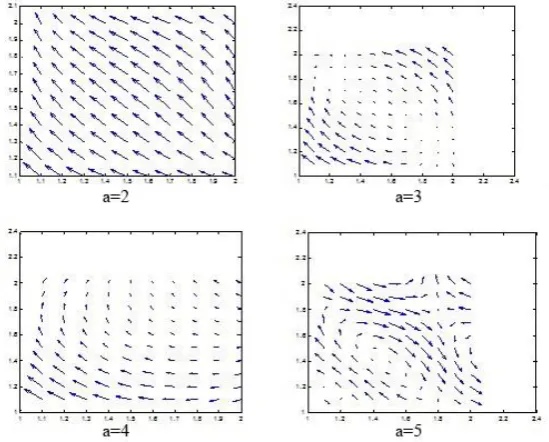
Fig.1 shows the change of flow field after truncation as the truncation radius gradually increases.

Figure 1. The change of flow field diagram with differenta.

It can be seen from Fig.1 that the truncated system basically maintains the flow field characteristics of the original system. However, as the truncation radius increases, some singularities (such as saddle points, as can be seen from the figure) gradually appear in the truncated system. It can be concluded that the flow field of the original system is well restored after truncation, but simply increasing the truncation radius cannot improve the approximate accuracy. By selecting appropriate wave vectors, the truncated equation can guarantee the properties of the original NS equation to a large extent. That is to say, the linear term and the quadratic cross term such asxy can preserve the complexity of NS equation. Therefore, we take the ordinary differential equation in the following form

1 2 1,2 k a k _{k k} k k

   



Differential System Construction Methods for Complex Surface

11 12 13 14 15 16

21 22 23 24 25 26

31 32 33 34 35 36

x

y

x a a a a a a

z

y a a a a a a

xy

z a a a a a a

xz yz          _{ }   _       _{ }        _{ }      

. (4)

wherex y z, , are the coordinates of a surface in three-dimensional Euclidean space. We use the simplest first-order difference scheme, and the original system becomes as follows:

1 11 12 13 14 15 16

1 21 22 23 24 25 26

1 31 32 33 34 35 36

n n n n n n n n n n n n n n n x y

x x a a a a a a

z

y y t a a a a a a

x y

z z a a a a a a

x z y z              _{ }  _ _{ }  _{ }    _{ }  _       _{ }      

. (5)

LetAbe the coefficient matrix and





1 1

1 1

1 1

1 1 1 1

1 1 1 1

1 1 1 1

n n n n n n n x x y y z z X

x y x y

x z x z

y z y z

                             

and multiply both sides of this equation byXT.XXTis positive definite when the set of data points satisfies certain conditions. By multiplying both sides of this equation by the inverseXXTand we obtain the following equation:





2 1 1

1

2 1 1

2 1 1

n n

T T

n n

n n

x x x x

tA y y y y X XX

z z z z

           _   _  _{ }   

. (6)

In this form, tA can be solved. By plugging in the first point in the curve, the whole curve can be reconstructed through Eq. 5. The process of the differential system fitting method is as following:

Step 1. Get the surface points. Denoise and filter the data points.

Step 2. Use the presented differential system construction method to fitN primitive curve.

Step 3. Construct the overall description of the surface. Each primitive curve is represented by a corresponding parameter matrix, and the curves between the two primitive curves are obtained by the nonlinear homotopy method.

Experiment

Comparison of the Two Construction Methods

We sample data points of a rotor blade of a certain type of compressor as the original data for comparison. The data set includes 15 groups, and 2 of each group form a closed curve.

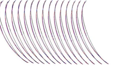
The fitting result pairs are shown in Fig.2. The red line shows the experimental data. The blue line and pink line respectively represent the fitting effect of the differential system under the first-order difference scheme and the second-order difference scheme. The green line represents the fitting effect of our method of differential system construction based on truncation. Obviously, the difference scheme basically does not affect the accuracy of fitting.

Figure 2. Two difference schemes of linear system and truncation system.

We fitted each set of leaves in the data. Matching the results, we find that the fitting method proposed in this paper performs obviously better than the general linear fitting method. To some extent, the truncation system represents the original NS system well. On the other hand, we can also see that the blade shape does follow the NS equation.

An Improved Method

The velocity distribution for each point in the flow field is inconsistent. In order to fit more closely to the flow field, we require that the velocity field of the two systems at the scatter position also fit well. In the previous experiment of rotor blade fitting, the time from the data point to the adjacent data points is taken as a unit step, and the step length between every two adjacent points is considered to be certain. By observing the original data points, we find that there are fewer sampling points in the places where the curve curvature is large, and more sampling points in the places where the curve curvature is small. Therefore, the method of selecting the step size mentioned above is to consider that the fluid has a high velocity at the place with a smooth curve and a low velocity at the place with a steep curve. If the step size in the fitting process is modified, the velocity distribution mode of the fitted system is changed. In the constant velocity field, the velocity is identical at every point, and the direction is not the same. The qualified formula is modified as follows:

1 1

1 2

i i i i

i i

X X X X

A

X X

s

 



 



 . (7)

wheresis the entire length of arc length. We select the scatter point on the stator blade for fitting and compare it with the original linear fitting result.

In Fig.3, the red line represents the original data, the black line is the fitted curve before the step size improvement, and the blue line is the fitted curve after the improvement. Obviously, the improved method is better than the original method in curve fitting. It also shows that the streamline velocity is almost constant on the stator blade.

Conclusion and Future Work

We have proposed a construction method of differential system for complex surface based on aerodynamic design. Through introducing a high-dimensional truncation of Navier-Stokes equations, we transform the complex partial differential system into an ordinary one. On the premise of preserving the local nature of the solutions, we propose a new method for selecting wave vector sets to simplify the expression of the equations. Finally, we use the truncated ordinary differential system to describe the shape of complex surface. Furthermore, we improved the step selection in the fitting method. Experimental results show that our method is superior to the traditional linear fitting method. Our future work may focus on the optimization and manufacture of compressor blades integrated with this model.

Acknowledgement

This work is supported by National Key Research and Development Program of China (Grant No.2018YFB1107402) and NSFC (Grant No.11290141).

References

[1] Boldrighini C, Franceschini V. A five-dimensional truncation of the plane incompressible Navier-Stokes equations[J]. Communications in Mathematical Physics, 1979, 64(2): 159-170.

[2] Lorenz E N. The mechanics of vacillation[J]. Journal of the atmospheric sciences, 1963, 20(5): 448-465.

[3] Bloor M I G, Wilson M J. Generating blend surfaces using partial differential equations[J]. Computer-Aided Design, 1989, 21(3): 165-171.

[4] Bloor M I G, Wilson M J. Using partial differential equations to generate free-form surfaces[J]. Computer-Aided Design, 1990, 22(4): 202-212.

[5] Ugail H, Bloor M I G, Wilson M J. Techniques for interactive design using the PDE method[J]. ACM Transactions on Graphics (TOG), 1999, 18(2): 195-212.

[6] Du H, Qin H. Dynamic PDE surfaces with flexible and general geometric constraints[C]//Proceedings the Eighth Pacific Conference on Computer Graphics and Applications. IEEE, 2000: 213-447.

[7] Castro G G, Ugail H, Willis P, et al. A survey of partial differential equations in geometric design[J]. The Visual Computer, 2008, 24(3): 213-225.

[8] May R M. Simple mathematical models with very complicated dynamics[M]//The Theory of Chaotic Attractors. Springer, New York, NY, 2004: 85-93.

[9] Franceschini V, Zanasi R. Three-dimensional Navier-Stokes equations truncated on a torus[J]. Nonlinearity, 1992, 5(1): 189.

[11] Jones D A, Titi E S. Upper bounds on the number of determining modes, nodes, and volume elements for the Navier-Stokes equations[J]. Indiana University Mathematics Journal, 1993: 875-887.

[12] Foias C, Manley O P, Temam R, et al. Number of modes governing two-dimensional viscous, incompressible flows[J]. Physical Review Letters, 1983, 50(14): 1031.

[13] Fang H P. Behavior of N-Mode Truncated Navier-Stokes Equations with External Force Acting on Various Modes[J]. Communications in Theoretical Physics, 1994, 21(3): 257.

[14] Jones D A, Titi E S. On the number of determining nodes for the 2D Navier-Stokes equations[J]. Journal of mathematical analysis and applications, 1992, 168(1): 72-88.