Stochastic Model of a Cold Stand by System with Waiting for Arrival & Treatment of Server

http://dx.doi.org/10.4236/ajor.2016.64031

Stochastic Model of a Cold-Stand by

System with Waiting for

Arrival & Treatment of Server

Rohtash K. Bhardwaj, Ravinder Singh

Department of Statistics, Punjabi University, Patiala, India

Received 29 February 2016; accepted 18 July 2016; published 21 July 2016

Copyright © 2016 by authors and Scientific Research Publishing Inc.

This work is licensed under the Creative Commons Attribution International License (CC BY).

http://creativecommons.org/licenses/by/4.0/

Abstract

The service facility or server is the key constituent to keep a system operational for desired period of time. As any eventuality with the system necessitates immediate presence of it (server) so the time point of arrival and treatment of server significantly affects the system performance. This paper works out the steady state behavior of a cold standby system equipped with two similar units and a server with elapsed arrival and treatment times following general probability distri-butions. It practices the theory of semi-Markov processes, regenerative point technique and Lap-lace transforms to derive the expressions for state transition probabilities, mean sojourn times, mean time to system failure, system availability, server busy period and expected frequencies of repairs and treatments. The profit function is also developed taking different costs and revenue in to account. For tracing wider applicability of the model for different reliability and cost-effective systems, a particular case study is also presented as an illustration.

Keywords

Stochastic Model, Cold-Standby System, Server Failure, Regenerative Point, Arrival and Treatment Times

1. Introduction

per-formance both in terms of reliability as well as availability, the proviso of standby redundancy is widely consi-dered in the literature [15]-[19]. The repairable systems are described with the feature that as soon as any com-ponent/unit fails it is either repaired or replaced by the service facility. So the service facility plays a key role in keeping a repairable system operational for longer period of time. In such cases, the failure of service facility interrupts the system performance in terms of availability, reliability and profit [20]-[22]. So the modeling of ar-rival and treatment times of server becomes essentially important to marginalize the loss due to system down time. Keeping these facts in view, the present paper investigates a cold-standby system taking account of wait-ing time for arrival and treatment of server subject to failure. The semi-Markov processes and regenerative point technique are used to obtain following measures of system performance in steady state:

a) Transition probabilities and mean sojourn times in different states. b) MTSF and reliability of the system.

c) System availability. d) Server busy period.

e) Expected number of repairs and treatments. f) And expected profit.

2. System Assumptions & States Description

2.1. Assumptions

To provide ease to the computational work, the model is developed using the following set of assumptions: a) The model consists of two identical units. Initially, one unit is in operation and another as cold-standby. b) The unit in standby mode can’t fail.

c) Upon failure of the operative unit the standby becomes operative instantly.

d) All the failures are repairable to be repaired by the server but the server takes some time to arrive. e) The server may fail while working but curable.

f) The server restoration subjects to treatment with some elapsed time. g) All the repairs, treatments and switching are perfect.

h) The system works as long as at least one unit remains working. i) All the random variables are assumed to be statistically independent.

j) All the random variables follow general probability distribution with different distribution functions.

2.2. States of the System

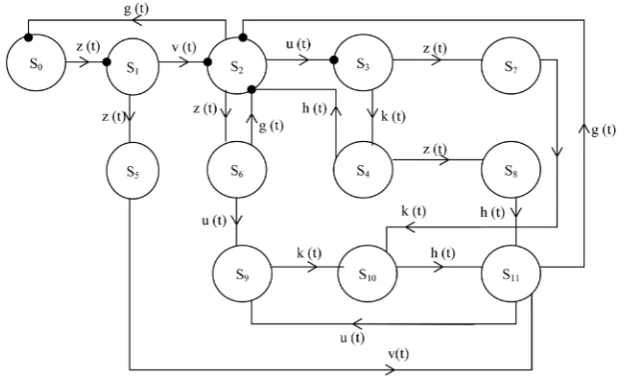
The system model comprises of regenerative and non-regenerative states. The states S i_i, =0,1,, 3 are rege-nerative whereas the states S ii, =4, 5,,11 are non-regenerative. The detailed description of all possible states is as follows:

0: System up. One unit is operating and another in cold standby mode.

S

1: System up. One unit is operating and another failed waiting for repair.

S

2: System up. One unit is operating and another under repair.

S

3: System up. One unit is operating, another waiting for repair and server waiting for treatment.

S

4: System up. One unit is operating, other continuously waiting for repair and server under treatment.

S

5: System down. Both units waiting for repair and server not present.

S

6: System down. One unit under continuous repair and another waiting for repair.

S

7: System down. Both units waiting for repair and the server continuously waiting for treatment.

S

8: System down. Both units waiting for repair/ continuous repair and server under continuous treatment.

S

9: System down. Both units waiting/continuously waiting for repair and server under treatment.

S

10: System down. Both units continuously waiting for repair and server under treatment.

S

11: System down. One unit under repair, another continuously waiting for repair.

S

3. Notations & Acronyms

( )

{

The system is in up-state at instant | the system entered regenerative state at 0 .

}

i

A t =P t i t=

( )

{

The server is busy in repair at an instant | the system entered regenerative state at 0 .

}

i

( )

Expected number of repairs of units in 0,

(

]

given that the system entered regenerative state at

i

D t = t i

0.

t=

( )

Expected number of server's treatments in 0, given that the system entered regenerative state at

(

]

i

T t = t i

0.

t=

( )

{

System is initially up in is up at without visiting other

}

.

i i j

M t =P S ∈E t S ∈E

( ) ( )

/

z t Z t : pdf/cdf of failure time of the unit.

( ) ( )

/

u t U t : pdf/cdfof failure time of the server.

( ) ( )

/

g t G t : pdf/cdf of repair time of the failed unit.

( ) ( )

/

h t H t : pdf/cdf of the treatment time of the server.

( ) ( )

/

k t K t : pdf/cdf of the waiting time of the server for treatment.

( ) ( )

/

v t V t : pdf/cdf of the arrival time of the server.

( )

( )

, / ,

i j i j

q t Q t : pdf/cdf of direct transition time from a regenerative state i to a regenerative state j without visiting any other regenerative state.

( )

( )

, . / , . i j k i j k

q t Q t : pdf/cdf of first passage time from a regenerative state i to a regenerative state j or to a failed state j visiting state k once in (0, t].

( )

( )

, . , / , . , i j k r i j k r

q t Q t : pdf/cdf of first passage time from regenerative state i to a regenerative state j or to a failed state j visiting state k, r once in (0, t].

( )

( )

, . , , / , . , , i j k r s i j k r s

q t Q t : pdf/cdf of first passage time from regenerative state i to a regenerative state j or to a failed state j visiting state k, r and s once in (0, t].

( )

i

W t : Probability that the server is busy in the state Si up to time ‘t’ without making any transition to any other regenerative state or returning to the same state via one or more non-regenerative states.

, i j

m : Contribution to mean sojourn time (µi) in state Si when system transit directly to state j.

{ }

, . n i j k lmn m

 : Contribution to mean sojourn time (µi) in state Siwhen system transit to state j via k and n times between , , ,l m n

(s)/(c): Stieltjes convolution/Laplace convolution.

~: Laplace Stieltjes Transform (LST). * Laplace Transform (LT).

I

L− : Inverse Laplace Transform.

4. The Model Development

4.1. The State Transition Diagram

Taking account of all possible transitions and the re-generative points a system schematic state transition dia-gram is constructed as given in Figure 1. The solid dots denote the regenerative epochs for various states of the model. The probability density functions of various random variables are also shown inFigure 1.

4.2. State Transition Probabilities

Simple probabilistic considerations, yields the following expressions for the non-zero elements

( )

₀

( )

d

ij ij ij

p =Q ∞ =

∫

∞q t t (1)

( )

( ) ( )

( ) ( )

_{( )}

( )

( )

0,1 ₀ d , 1,2 ₀ d , 1,5 ₀ d , _{1,2.5, 11,9,10}n 1,5 5,11 11,2,

p =

∫

∞z t t p =

∫

∞v t Z t t p =

∫

∞z t V t t p = p c p c p

( ) ( ) ( )

2,0 ₀ d ,

p =

∫

∞g t Z t U t t _2,3

( ) ( ) ( )

_2,6

( ) ( ) ( )

0 d , 0 d ,

p =

∫

∞u t Z t G t t p =

∫

∞z t G t U t t

( )

_{( )}

( )

( )

( )

( )

2,2.6 2,6 6,2, ,_{2,2.6, 9,10,11}n 2,6 6,9 9,10 10,11 11,2

p = p c p p =p c p c p c p c p

( ) ( )

( ) ( )

( )

3,4 ₀ d , d ,3,7 ₀ 3,2.4 3,4 4,2,

[image:4.595.158.476.85.279.2]

Figure 1. The schematic system state transition diagram.

( ) 3,4

( )

4,8

( )

8,11

( )

11,2

3,2.4,8, 11,9,10n ,

p = p c p c p c p p_{3,2.7, 10,11,9( )}n = p3,7

( )

c p7,10

( )

c p10,11

( )

c p11,2,

( )

( ) ( )

( ) ( )

3,8.4 3,4 4,8, 4,2 ₀ d , 4,8 ₀ d ,

p = p c p p =

∫

∞h t Z t t p =

∫

∞z t H t t

( )

( ) ( )

( ) ( )

( )

5,11 ₀ d , 6,9 ₀ d , 6,2 ₀ d , 7,10 ₀ d ,

p =

∫

∞v t t p =

∫

∞u t G t t p =

∫

∞g t U t t p =

∫

∞k t t

( )

( )

( )

8,11 ₀ d , 9,10 ₀ d , 10,11 ₀ d ,

p =

∫

∞h t t p =

∫

∞k t t p =

∫

∞h t t

( ) ( )

( ) ( )

11,2 ₀ d , 11,9 ₀ d

p =

∫

∞g t U t t p =

∫

∞u t G t t

For these Transition Probabilities, it can be verified that

( ) ( )

( ) ( )

0,1 1,2 1,5 1,2 _{1,2.5, 11,9,10} 2,0 2,3 2,6 2,0 2,3 2,2.6 _{2,2.6, 9,10,11}

3,4 3,7 3,2.4 _{3,2.4,8, 11,9,10 3,2.7, 10,11,9} 3,8.4 3,2.4 3,7 4,8 4,2

5,11 6,2 6,9 7,10 8,11 9,10 1

n n

n n

p p p p p p p p p p p p

p p p p p p p p p p

p p p p p p p

= + = + = + + = + + +

= + = + + = + + = +

= = + = = = = 0,11= p11,2+p11,9=1

4.3. Mean Sojourn Times

The Mean sojourn time µi in state Si are given by:

( )

₀

(

)

d ; 0,1, 2, 3.

i E t P T t t i

µ = =

_∫

∞ > = (2)

( )

( ) ( )

( ) ( ) ( )

( ) ( )

0 ₀ Z t d ,t 1 ₀V t Z t , 2 ₀ Z t U t G t d ,t 3 ₀ K t Z t dt

µ =

_∫

∞ µ =

_∫

∞ µ =

_∫

∞ µ =

_∫

∞

The unconditional mean time taken by the system to transit from any state Si when time is counted from epoch at entrance into state Sjis stated as:

( )

*

( )

d 0

ij ij ij

m =

∫

t Q t = −q′

( )

0,1 0, , 1,2 1,5 1 1,2 _{1,2.5, 11,9,10}n 1, 2,0 2,3 2,6 2,

m =µ m +m =µ m +m =µ′ m +m +m =µ

( )

2,0 2,3 2,2.6 _{2,2.6, 9,10,11}n 2, ,3,4 3,7 3

m +m +m +m =µ′ m +m =µ

( ) ( )

3,2.4 _{3,2.4,8, 11,9,10}n _{3,2.7, 10,11,9}n 3, 3,8.4 3,2.4 3,7 3,

4,8 4,2 4, ,5,11 5 6,2 6,9 6, 7,10 7,

m +m =µ m =µ m +m =µ m =µ

8,11 8, , , 9,10 9 10,11 10 11,2 11,9 11

m =µ m =µ m =µ m +m =µ

5. Stochastic Analysis

5.1. Reliability Measure

Let φ_i

( )

t be the c.d.f of the first passage time from regenerative state Si to a failed state. Regarding the failed state as absorbing state, we have the following recursive relations for φi

( )

t :

( )

{

,

( )

, .

( )

, .

( )

, .

( )

}

( ) ( )

,

( )

; 0,1, 2, 3

i i j i j k i j kl i j klm j i f

j f

t Q t Q t Q t Q t c t Q t i

φ =

∑

+ + + + _ φ +

∑

= (3)

where Sj is an un-failed regenerative state to which the given regenerative state Si can transit and Sk is failed state to which the state Sican transit directly.

Taking LST of Equation (3) and solving for φ0

( )

s , we get MTSF as follows:

( )

{

( )

}

(

)

(

)

0 *

0 0

0 1 2,3 3,2.4 1 2 2,3 1,2

0,1 1,2 2,0 2,3 3,2.4 1 lim lim 1 1 s s s

MTSF R s

s

p p p p

p p p p p

φ

µ µ µ µ

→ →  −    = =     ′′   + _ − _+ + = − − 

The reliability R(t) is given by

( )

₁

{

_*

( )

}

₁

{

1 0

( )

s

}

R t L R s L

s φ − − _ − _ = =     

5.2. Economic Measures

Let the system entered the regenerative state Si at t = 0. Considering Sj as a regenerative state to which the given regenerative state Si transits, the recursive relations for various profit measures in (0, t] are given as follow:

( )

( )

{

,

( )

, .

{

, .

( )

, .

( )

}

}

( ) ( )

; 0,1, 2, 3

i i i j i j kl i j k i j kl j

j

A t =M t +

∑

q t +δ _ q t +q t + c A t i= (4)

( )

( )

{

,

( )

, , ,

{

, .

( )

, .

( )

}

}

( ) ( )

; 0,1, 2, 3

i i i j i j k l i j k i j kl j

i

B t =W t +

∑

q t +δ _ q t +q t + c B t i= (5)

( )

{

( )

( )

}

{

, , . , . , .

}

( )

{

( )

}

( ) ; 0,1, 2, 3

i i j i j kl i j k i j kl j j

j

D t =

∑

Q t +δ _ Q t +Q t + s δ +D t i= (6)

( )

{

,

( )

, .

{

, .

( )

, .

( )

}

}

( )

{

( )

}

; 0,1, 2, 3

i i j i j kl i j k i j kl j j

j

T t =

∑

Q t +δ _ Q t +Q t + s δ +T t i= (7)

Here, 1; if there is a repair/treatment from to 0; Otherwise

i j

j

S S

δ _{= } 

And , . . , ,

1; if there is a transition from to via

0; Otherwise

i j k l

i j k l

S S S

δ _{= } 

 

Using LT/ LST, of Equations (4)-(7) and solving we get the results in steady state as below:

( )

(

)

(

0 1 0,1

)

2,0 2 3 2,3

*

0 0 _.

0

0 1 0,1 2,0 2 3 2,3 lim

s

p p p

A sA s

p p p

µ µ µ µ

µ µ µ µ

→ + + + = = ′ ′ + + +

( )

( )

(

)

* 2 *

0 0 _.

0

0 1 0,1 2,0 2 3 2,3

0 lim

s

W B sB s

p p p

µ µ µ µ

→

= =

′ ′

( )

₍

0,1 2,3

₎

3,2.4 0,1 2,0 1,2

0 ₀ 0 .

0 1 0,1 2,0 2 3 2,3

1 lim

s

p p p p p p D sD s

p p p

µ µ µ µ

→

− −

= =

′ ′

+ + +



( )

₍

2,2.4

₎

2,3 0,1

0 0 _.

0

0 1 0,1 2,0 2 3 2,3

lim

s

p p p T sT s

p p p

µ µ µ µ

→

= =

′ ′

+ + +



Further, using the values of above performance measures, the profit incurred to the system model in steady state is given as below.

Profit=Total Revenue generated−Total Expenses occured

0 o o 1 o 2 o 3 o

P =K A −C B −C D −C T

0 Revenue per unit up time of the system.

K =

1 Cost per unit time for which server is busy.

C =

2 Cost per unit time repair of the uint.

C =

3 Cost per unit time server treatment

C = and A B D T0, 0, 0, 0 are already defined.

6. Example (Particular Case of Exponential Distribution)

For the sake of convenience, let us suppose all the random variables follow the exponential distribution with the probability density functions given below.

( )

e t,

( )

e t,

( )

e t,

( )

e t,

( )

e t,

( )

e t

z t =λ −λ v t =ψ −ψ g t =α −α u t =γ −γ k t =ξ −ξ h t =β −β

We assume some particular values for various time rates and costs i.e.

Failure rate of server (γ) = 0.02 per unit time, Failure rate of unit (λ) = 0.008 per unit time. Repair rate of unit (α) = 0.3 per unit time, Treatment rate of server (β) = 0.05 per unit time. Server arrival rate (ψ) = 0.08 per unit time, Waiting treatment time (ξ) = 0.08 per unit time. And K0=20 ,K C1=500,C2=300,C3=900.

For this, we obtained the values for different measures of system performance as follows: MTSF = 1110.909 unit time, Availability = 0.977238, Busy period of server = 0.023716, Expected number of repairs = 0.000918, Expected number of treatments =0.000364 and System profit = 19532.31.

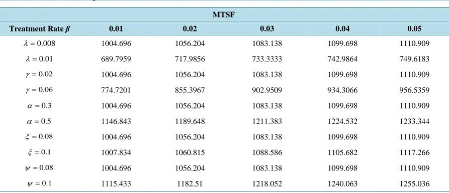
[image:6.595.90.538.527.720.2]

The detailed results are given in tabular form. Here Tables 1-3 respectively, illustrate the effect of server treatment rate for various combinations of parameters on Mean Time to System Failure (MTSF), availability and profit assuming

(

λ=0.008,γ =0.02,α=0.3,ξ =0.08,ψ =0.08

)

.

Table 1. Effect of various parameters on MTSF.

MTSF

Treatment Rate β 0.01 0.02 0.03 0.04 0.05

0.008

λ= 1004.696 1056.204 1083.138 1099.698 1110.909 0.01

λ= 689.7959 717.9856 733.3333 742.9864 749.6183

0.02

γ= 1004.696 1056.204 1083.138 1099.698 1110.909

0.06

γ= 774.7201 855.3967 902.9509 934.3066 956.5359 0.3

α= 1004.696 1056.204 1083.138 1099.698 1110.909 0.5

α= 1146.843 1189.648 1211.383 1224.532 1233.344

0.08

ξ= 1004.696 1056.204 1083.138 1099.698 1110.909

0.1

ξ= 1007.834 1060.815 1088.586 1105.682 1117.266

0.08

ψ= 1004.696 1056.204 1083.138 1099.698 1110.909

0.1

[image:7.595.85.541.104.347.2]

Table 2. Effect of various parameters on system availability.

Availability

Treatment rate β 0.01 0.02 0.03 0.04 0.05

0.008

λ= 0.936585 0.961641 0.970256 0.974611 0.977238

0.01

λ= 0.91928 0.949691 0.960247 0.965604 0.968842

0.02

γ= 0.936585 0.961641 0.970256 0.974611 0.977238

0.06

γ= 0.840416 0.908284 0.932934 0.94563 0.953361

0.3

α= 0.936585 0.961641 0.970256 0.974611 0.977238

0.5

α= 0.958533 0.973861 0.979065 0.981685 0.983261

0.08

ξ= 0.936585 0.961641 0.970256 0.974611 0.977238

0.1

ξ= 0.936889 0.961972 0.970594 0.974952 0.977581

0.08

ψ= 0.936585 0.961641 0.970256 0.974611 0.977238

0.1

[image:7.595.89.538.331.532.2]

ψ = 0.939355 0.964577 0.97325 0.977634 0.98028

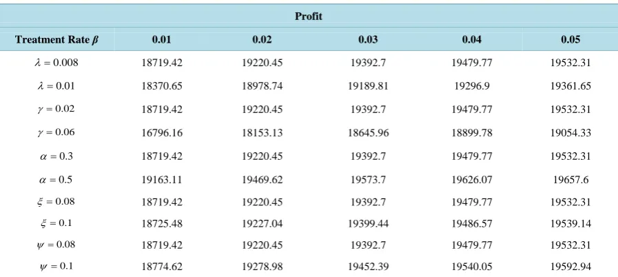
Table 3. Effect of various parameters on system profit.

Profit

Treatment Rate β 0.01 0.02 0.03 0.04 0.05

0.008

λ= 18719.42 19220.45 19392.7 19479.77 19532.31

0.01

λ= 18370.65 18978.74 19189.81 19296.9 19361.65

0.02

γ= 18719.42 19220.45 19392.7 19479.77 19532.31

0.06

γ= 16796.16 18153.13 18645.96 18899.78 19054.33

0.3

α= 18719.42 19220.45 19392.7 19479.77 19532.31

0.5

α= 19163.11 19469.62 19573.7 19626.07 19657.6

0.08

ξ= 18719.42 19220.45 19392.7 19479.77 19532.31

0.1

ξ= 18725.48 19227.04 19399.44 19486.57 19539.14

0.08

ψ= 18719.42 19220.45 19392.7 19479.77 19532.31

0.1

ψ= 18774.62 19278.98 19452.39 19540.05 19592.94

7. Discussion and Concluding Remark

A stochastic model for a repairable cold standby system, with waiting arrival and treatment times of server, is discussed in this paper. The theory of semi-Markov process and regenerative point technique is used to derive expressions for measures of reliability and profit. An example is given under the setup of exponential distribu-tion by assigning distinct values to various parameters and costs considered for the system model. The further numerical results (as given in Tables 1-3) indicate that MTSF, availability and the profit rise with increasing server treatment rate (β), repair rate of units (α) and server arrival time (ψ) but the trend reverts with increasing the failure rates of server (γ) and unit (λ). The persisting trend reveals that the waiting arrival and treatment times impact a lot on the system performance. Therefore, the study re-iterates the practicalities that a cold standby system served by a repairable server can be kept reliable and profitable by:

1) Using standard units with low failure rates. 2) Deploying efficient server with high repair rates. 3) Planning for higher arrival rate of server and,

The re-iteration of the true facts evidently proves the acceptability of the probabilistic model developed in this paper. The study may be inspiring and useful for system planners and reliability engineers for developing highly reliable and profitable systems to earn users’ satisfaction.

The study finds its application in diverse areas such as power generating systems with standby reservoirs, communication systems with redundant channels, remote sensing systems with alternate power backups etc.

Acknowledgements

This work is a part of Major Research Project F. N. 42-34/2013(SR) financially supported by UGC under MHRD, Govt. of India. The authors are grateful to anonymous referee for their valuable comments and sugges-tions.

References

[1] Osaki S. and Nakagawa T. (1976) Bibliography for Reliability and Availability of Stochastic Systems. IEEE Transac-tions on Reliability, 4, 284-287. http://dx.doi.org/10.1109/TR.1976.5219999

[2] Osaki, S. (1985) Stochastic System Reliability Modeling. World Scientific, Singapore City.

http://dx.doi.org/10.1142/0164

[3] Lindqvist, B.H. (1987) Monotone and Associated Markov Chains, with Applications to Reliability Theory. Journal of Applied Probability, 24,679-695. http://dx.doi.org/10.2307/3214099

[4] Aven, T. (1990) Availability Formulae for Standby Systems of Similar Units That Are Preventively Maintained. IEEE Transactions on Reliability, 39,603-606. http://dx.doi.org/10.1109/24.61319

[5] Birolini, A. (1994) Quality and Reliability of Technical Systems. Springer, New York.

http://dx.doi.org/10.1007/978-3-662-02970-1

[6] Gnedenko, B. and Ushakov, I.A. (1995) Probabilistic Reliability Engineering. Wiley Sons, New York. [7] Ebeling, C.E. (1997) An Introduction to Reliability and Maintainability Engineering. McGraw-Hill, Boston.

[8] Rausand, M. and Høyland, A. (2004) System Reliability Theory: Models, Statistical Methods, and Applications. 2nd Ed, John Wiley & Sons, Hoboken.

[9] Smith, W.L. (1958) Renewal Theory and Its Ramifications. Journal of the Royal Statistical Society, 20, 243-302.

[10] Pyke, R. (1961) Markov Renewal Processes: Definitions and Preliminary Properties. The Annals of Mathematical Sta-tistics, 32,1231-1242. http://dx.doi.org/10.1214/aoms/1177704863

[11] Limnios, N. and Oprişan, G. (2001) Semi-Markov Processes and Reliability; Statistics for Industry and Technology. Birkhäuser, Boston.

[12] Malefaki, S., Limnios, N. and Dersin, P. (2014) Reliability of Maintained Systems under a SEMI-MARKOV SETTING. Reliability Engineering & System Safety, 131, 282-290. http://dx.doi.org/10.1016/j.ress.2014.05.003

[13] Bhardwaj, R.K. and Singh, R. (2014) Semi Markov Approach for Asymptotic Performance Analysis of a Standby Sys-tem with Server Failure. International Journal of Computer Applications, 98,9-14.

[14] Bhardwaj, R.K. and Singh, R. (2015) Semi-Markov Model of a Standby System with General Distribution of Arrival and Failure Times of Server. American Journal of Applied Mathematics and Statistics, 3, 105-110.

[15] Gupta, S.M., Jaiswal, N.K. and Goel, L.R. (1982) Reliability Analysis of a Two-Unit Cold Standby Redundant System with Two Operating Modes. Microelectronics Reliability, 22, 747-758.

http://dx.doi.org/10.1016/S0026-2714(82)80191-1

[16] Subramanian, R. and Anantharaman, V. (1995) Reliability Analysis of a Complex Standby Redundant Systems. Relia-bility Engineering & System Safety, 48, 57-70. http://dx.doi.org/10.1016/0951-8320(94)00073-W

[17] Bhardwaj, R.K. and Malik, S.C. (2011) Asymptotic Performance Analysis of 2oo3 Cold Standby System with Con-strained Repair and Arbitrary Distributed Inspection Time. International Journal of Applied Engineering Research, 6, 1493-1502.

[18] Bhardwaj, R.K. and Kaur, K. (2014) Reliability and Profit Analysis of a Redundant System with Possible Renewal of Standby Subject to Inspection. International Journal of Statistics and Reliability Engineering, 1, 36-46.

[19] Bhardwaj, R.K., Kaur, K. and Malik, S.C. (2015) Stochastic Modeling of a System with Maintenance and Replacement of Standby Subject to Inspection. American Journal of Theoretical and Applied Statistics, 4, 339-346.

http://dx.doi.org/10.11648/j.ajtas.20150405.14

[21] Bhardwaj, R.K. and Singh, R. (2015) An Inspection-Repair-Replacement Model of a Stochastic Standby System with Server Failure. Mathematics in Engineering, Science & Aerospace (MESA), 6,191-203.

[22] Bhardwaj, R.K. and Singh, R. (2015) A Cold-Standby System with Server Failure and Delayed Treatment. Interna-tional Journal of Computer Applications, 124,31-36. http://dx.doi.org/10.5120/ijca2015905823

Submit or recommend next manuscript to SCIRP and we will provide best service for you:

Accepting pre-submission inquiries through Email, Facebook, LinkedIn, Twitter, etc. A wide selection of journals (inclusive of 9 subjects, more than 200 journals) Providing 24-hour high-quality service

User-friendly online submission system Fair and swift peer-review system

Efficient typesetting and proofreading procedure

Display of the result of downloads and visits, as well as the number of cited articles Maximum dissemination of your research work