Density Based Regression for Inhomogeneous Data: Application to Lottery Experiments

Munich Personal RePEc Archive

Density Based Regression for

Inhomogeneous Data: Application to

Lottery Experiments

Kontek, Krzysztof

Artal Investments

21 April 2010

Online at

https://mpra.ub.uni-muenchen.de/22268/

Krzysztof Kontek1

Artal Investments, Warsaw2

This paper presents a regression procedure for inhomogeneous data characterized by

varying variance, skewness and kurtosis or by an unequal amount of data over the estimation

domain. The concept is based first on the estimation of the densities of an observed variable

for given values of explanatory variable(s). These density functions are then used to estimate

the relation between all the variables. The mean, quantile (including median) and mode re&

gression estimators are proposed, with the last one appearing to be the maximum likelihood

estimator in the density based approach. The paper demonstrates the advantages of the pro&

posed methodology, which eliminates most of the estimation problems arising from data in&

homogeneity. These include the computational inconveniences of the standard quantile and

mode regression techniques. The proposed methodology, when applied to lottery experiments,

makes it possible to confirm and to extend the previously presented conclusion (Kontek,

2010) that lottery valuations are only nonlinear with respect to probability when medians and

means are considered. Such nonlinearity disappears once modes are considered. This means

that the most likely behavior of a group is fully rational. The regression procedure presented

in this paper is, however, very general and may be applied in many other cases of data inho&

mogeneity and not just lottery experiments.

: C01, C13, C16, C21, C46, C51, C81, C91, D03, D81, D87

Density Distribution; Least Squares, Quantile, Median, Mode, Maximum Likeli&

hood Estimators; Lottery experiments; Relative Utility Function; Prospect Theory.

1

The author is grateful to Stefan Traub from the Department of Economics, University of Bremen, Ulrich Schmidt from the Department of Economics, University of Kiel and Katarzyna Idzikowska from the Center of Economic Psychology and Decision Sciences, Kozminski University, Warsaw, for making the results of their experiments available. This paper would never have been written without their data.

2

!"

!"!" There are at least three ways in which data can be inhomogeneous. The first, fre& quently referred to as heterogeneity in the micro&economics literature, is encountered when

the object or system described consists of multiple items having a large number of structural

variations.

The second type is when the observed variable changes its properties over the estima&

tion domain. An example of this is heteroskedasticity, meaning that variance varies over time.

This type of inhomogeneity is, however, broader in meaning as higher moments of the distri&

bution (in particular skewness and kurtosis) may vary as well. An example of this is changes

in stock market indexes, which are usually negatively skewed during declines and positively

skewed during gains. In this paper, the term inhomogeneity refers to this second type of in&

homogeneity unless otherwise stated.

The third type of inhomogeneity is encountered when the data are not uniformly dis&

tributed in the estimation domain. This can occur when there are different amounts of data for

given values of explanatory variables and/or when the distribution of explanatory variable

values is non&uniform. For example, the amount of data on hourly wages can differ for differ&

ent values of the explanatory variable “Years of Schooling” (see Cameron, Trivedi, 2005,

Figure 9.3). Obviously this type of inhomogeneity can result from the nature of the phenome&

non under observation and can be deliberate in experiments as in the case of stratified sam&

pling.

All these types of inhomogeneity have to be carefully checked and addressed using

proper econometric methods in order to derive the correct relationships between the observed

and explanatory variables.

!"#" Each type of data inhomogeneity presented above is encountered in experiments determining the certainty equivalents of lotteries. This was considered in detail in another

paper by Kontek (2010), although the term “inhomogeneity” did not appear there.

To recapitulate, certainty equivalents are typically determined in lottery experiments

for several combinations of outcomes and for several probabilities of winning. A wide range

of certainty equivalent values was observed for specific probabilities in two analyzed sets of

data. This points to very diverse risk attitudes among the examined subjects. Different risk

attitudes were stated earlier by Tversky and Kahneman (1992) and by other researchers.

substantially with probability. The most striking results were observed for skewness. The data

are positively skewed for low probabilities, negatively skewed for high probabilities and not

skewed for medium probabilities. These results point to the second type of inhomogeneity

described in point 1.1.

Finally, different numbers of lotteries are examined for specific probabilities in every

set of data under consideration. Moreover, those probabilities are non&uniformly distributed in

the range [0,1]. This is an example of the third type of inhomogeneity described in point 1.1.

!"$" Kontek (2010) presented a wide range of regression methods in use for lottery ex& perimental data. These include standard least squares (mean), quantile (including median),

and mode estimators, all performed parametrically and nonparametrically.

Despite presenting several important conclusions, standard regression methods were

not able to dispel all of the doubts regarding the interpretation of the obtained results. The

standard procedures assume variance to be constant over the estimation domain. Varying

variance, or heteroskedasticity, requires more advanced procedures like weighted, generalized

or feasible generalized least squares estimators (Cameron, Trivedi, 2005). However, the prob&

lem of varying skewness or kurtosis is not considered even in the advanced textbooks on re&

gression methods as in the one mentioned above. This makes it difficult to predict how the

stated inhomogeneity of the data will impact the estimation results. For example, in one of the

examined sets, the median and mode regression estimations are practically the same but the

mean estimation is different. As all these estimations should be different when the data are

skewed, this can raise some objections as to the result.

Additionally the standard median and (especially) mode estimators are characterized

by computational inconveniences, which may lead to difficulties in finding the global opti&

mum. This raises the question of whether, and if so how, these inconveniences might be over&

come. The important question of how to define the maximum likelihood estimator for the data

considered has also been left open.

!"%" In view of the above, a novel approach is proposed in this paper, an approach based on parametrical estimation of densities of certainty equivalents (observed variable) for

given probability values (explanatory variable). These density distributions are later used for

mean, quantile and mode estimations of the relationship between the two variables. As shown,

the proposed methodology results in the maximum likelihood estimator being the mode esti&

mator. The paper compares the regression results obtained using the proposed approach with

The paper demonstrates the advantages of the proposed methodology, which elimi&

nates most of the estimation problems resulting from the inhomogeneity of the data. These

include the computational problems of the standard quantile and mode regression estimators.

As the concept presented here is very general, it can easily be applied to other cases of data

inhomogeneity and is not limited to lottery experiments.

Clearly, this method cannot be used when there are few data points for each value of

the explanatory variable. One disadvantage of the proposed method is that determining the

data densities requires an intermediate step. The accuracy of the density estimation therefore

has a vital impact on the final result. Another disadvantage is the additional computation time

required. On the other hand, determining the distributions will speed up the regression proce&

dure considerably. This method additionally comes with the nice feature of being able to pre&

dict the error distribution before the regression procedure, as the data distributions are already

known.

!"&" The presented methodology, when applied to lottery experiments, makes it possi& ble to confirm and extend the previously presented conclusion that lottery valuations are only

nonlinear with respect to probability when medians and means are considered. Such nonlin&

earity is not confirmed by the mode (maximum likelihood) estimator. This means that the

most likely behavior of a group is fully rational.

To the best of the author’s knowledge, this is the first paper to present a true maximum

likelihood estimation for lottery experiments where “true” is to be understood as meaning

based on the properly defined distribution of the observed variable (the typically assumed

normal error distribution reduces the maximum likelihood to a standard least squares proce&

dure).

!"'" An extensive number of estimation methods presented in this and the former pa& per were made possible by using the relative utility model which, in contrast to the Prospect

Theory model, adopts a classical econometric approach to data description. This model is

briefly outlined in Point 2. Point 3 presents the data sets examined in the present research.

Point 4 demonstrates calculated densities of the relative certainty equivalents for given prob&

abilities, which are then used for mean (Point 5), quantile (Point 6), and mode (Point 7) re&

#" ( ) *

#"!" The relative utility model assumes a direct relationship between probability and the relative certainty equivalents for a two outcome lottery:

( )

,

p=Q r (2.1)

where p denotes probability, Q denotes a relative utility function, which should have the form

of a cumulative density function defined over the range [0,1], and r denotes the relative cer&

tainty equivalent defined as:

, ce A r

P A

− =

− (2.2)

where ce denotes the certainty equivalent, P = Max(x) is the maximum lottery outcome, and A

= Min(x) is the minimum lottery outcome. The relationship described by (2.2) ensures that r

assumes values from the range [0, 1], even in the case of lotteries with a risk free component.

#"#" As probability p is a single&variable function of the relative certainty equivalent r, r can be easily represented as a function of p:

( )

1

,

r=Q− p (2.3)

where Q1 is the inverse form of the relative utility function. Because there are certainty equi&

valents which are typically determined in experiments rather than probabilities, the inverse

form (2.3) of the relative utility function will be mostly used throughout the paper.

#"$" It is possible to propose several functional forms for the relative utility function Q. Beta distribution is the only one used in this paper, as it is the best known and most widely

used distribution defined over the interval [0,1]. Hence, the function Q is described using

Cumulative Beta Distribution as follows:

( )

(

; ,

)

,

p=Q r =I r

α β

(2.4)

where I denotes the regularized incomplete beta function. The curve is S&shaped for α > 1 and

β > 1, inversed S&shaped for 0 < α < 1 and 0 < β < 1, J&shaped for α > 1 and 0 < β < 1, and

inverse J&shaped for 0 < α < 1 and β > 1. For α = 1 and β = 1 the curve is linear. The inversed

form of (2.4) is:

( )

(

)

1 1

; , ,

r=Q− p =I− p

α β

(2.5)

where I1 denotes the inverse of the regularized incomplete beta function. More on the relative

$" +

$"!" Two data sets are considered in the present study.

Set 1 & the experimental data presented by Traub and Schmidt (2009), whose research con&

cerned the relationship between WTP (Willingness to Pay) and WTA (Willingness to Accept).

Twenty four subjects participated in the experiment. Only that subset of the data covering the

certainty equivalents of two outcome lotteries was used in further analyses.

Set 2 & the experimental data of Idzikowska (2009), whose research concerns the question of

whether the form in which probability is presented has any impact on the shape of the prob&

ability weighting function. Twenty five subjects participated in the experiment but some of

the responses were disregarded by Idzikowska on account of their inconsistency. The present

research uses that subset of the data related to experimentally learned probabilities.

$"#"It is noted that the amount of collected data differs for specific probabilities. This is shown in Tables 3.1 and 3.2.

Probability .15 .17 .20 .25 .30 .40 .50 .60 .65 .80 .85 .90 Total

No of data 24 24 48 48 72 24 144 48 24 96 24 24 600

, $"!" Number of data for Set 1.

Probability .01 .05 .10 .25 .50 .75 .90 .95 .99 Total

No of data 54 53 57 55 116 61 54 58 60 568

, $"#" Number of data for Set 2.

The greatest number of data in both sets exists for the probability of 0.5. Additionally,

the data count is pretty high in Set 1 for probabilities 0.8 and 0.3. This means that these data

can dominate the data concerning the remaining probabilities during the estimation procedure,

which can have undesirable effects. A similar example of inhomogeneity may be found in

Tversky and Kahneman’s data (1992), which is presented in Table 3.3.

Probability .01 .05 .10 .25 .50 .75 .90 .95 .99

No of lotteries 2 3 3 3 6 3 3 3 2

, $"$" Number of lotteries having the given probability of winning the main prize.

It should be obvious that determining the densities of the relative certainty equivalents

for given probabilities solves the problem of unequal amounts of data. There is one density

%" ( - . (

%"!" In order to estimate a density function, its functional form must first be specified. There are a few possibilities, although not as many as in the case of unbounded distributions.

As in the case of the relative utility function, we will concentrate further on beta distribution

and its generalization3.

%"!"!" Beta distribution (bt) is defined as:

(

)

(

)

1 1 ₁ ( ; , ) . , r r bt r B δ γ γ δ γ δ − − ₋ = (4.1)

%"!"#" There are several generalizations of beta distribution (Gupta, Nadarajah, 2004) with 3, 4 or even 5 parameters. It should be noted that the number of parameters here is not a

problem and need not be limited. This is because determining the density function is only an

intermediate result where high accuracy is of great importance. The most adequate seems to

be the generalization gbt of Libby and Novick (1982):

(

)

(

)

₍

₎

1 1 1 ( ; , , ) .

, _{1 1}

r r gbt r B _r δ γ γ γ δ λ γ δ λ

γ δ _λ

− − + − = − +     (4.2)

%"#" Knowing the density function allows the characteristic points of the distribution to be determined analytically. The mean value of the gbt is4_:

(

; , ,

)

,

Mean gbt r

γ δ λ

γ

ϕ

m

γ δ

= =

 

  ₊ (4.3)

where

(

)

2F1 1, ;1 ;1 ,

ϕ

=

δ

+ +

γ δ

−

λ

(4.4)

denotes the hypergeometric function. For λ = 1, (4.3) reduces to the known formula for the

mean value of the beta distribution:

(

; ,

)

.

Mean bt r

γ δ

γ

γ δ

=

 

  ₊ (4.5)

The gbt mode (and anti&mode) is given by:

3

γ, δ, and λ are used throughout the paper to denote the parameters of the density function, whereas α and β are used to describe the relative utility function. Distribution written with small letters like bt, gbt or d denote den& sity functions, whereas written with capital letters like GBT or D denote cumulative density functions.

4

(

)

(

₍

₎

)

(

)(

)

2

3 3 8 1 1

; , , .

4 1

Mode gbt x

γ δ λ

γ λ δ λ

γ λ δ λ

γ

λ

λ

+ + − + + − − − − =     ₋ ∓ (4.6)

For λ = 1, (4.6) reduces to:

(

; ,

)

1 , 2

Mode bt r

γ δ

γ

γ δ

− =

 

  _{+ −} (4.7)

which is the beta distribution mode. The cumulative generalized beta distribution is defined

as:

(

; , ,

)

₍

₎

; , ,

1 1

r

GBT r I

r

λ

γ δ λ

γ δ

λ

 

= _{ − +} _

  (4.8)

where I denotes the regularized incomplete beta function. For λ = 1, (4.8) simplifies to the

cumulative beta distribution:

(

; ,

)

(

; ,

)

.

BT r

γ δ

=I r

γ δ

(4.9)

After inverting (4.8), the gbt quantile can be determined from:

(

)

(

)

1 1 , ; , , , 1 ; , Quantile q gbt r

I q

γ δ λ

λ λ γ δ − =     − + (4.10)

which, for λ = 1, expresses the beta distribution quantile:

(

)

1

(

)

, ; , ; , .

Quantile q bt r_ γ δ _=I− q γ δ (4.11)

In the special case where q = 0.5, the gbt median is given by:

(

)

(

)

1 1 ; , , . 1 0.5; , Median gbt r

I

γ δ λ

λ λ γ δ − =     − + (4.12)

The gbt variance is given by:

(

)

{

(

) (

)

(

)

(

)

}

(

) (

)

(

)(

)

(

)

2 2

2

1 1 1

; , ,

1

1 1

1

Variance gbt r

m m m m

var,

γ

γ δ

γ δ

γ

δ

λ φ γ

λ ϕ

γ δ λ

γ δ

λ

γ

δ λ

λ

+ − + _ + + − _ + − =     _{+ −} − − + − − = = − (4.13)

(

)

(

) (

2

)

; , .

1

Variance bt r γ δ γ δ

γ δ γ δ

=

 

  _{+ + +} (4.14)

%"$" Estimating densities is commonly achieved using the maximum likelihood estima& tor. The likelihood principle involves choosing the parameter vector θ that maximizes the

likelihood of observing the actual sample. The likelihood function is expressed by LN(θ|y,x)

and is a function of θ given the data (y, x). Maximizing LN(θ) is equivalent to maximizing the

(conditional) log&likelihood function:

( )

(

)

1

ln ln | , ,

N

N i i

i

L θ d y x θ

=

=

∑

(4.15)

where d denotes a (conditional) density function. The log&likelihood function for gbt is:

(

) (

)

(

)

(

)

(

)

(

)

(

)

1 1

1

ln , , 1 ln 1 ln 1 ln ,

ln ln 1 1 ,

N N

N i i

i i

N

i i

L r r N B

N r

γ δ λ γ δ γ δ

γ λ γ δ λ

= =

=

= − + − − −

+ − + _ − + _

∑

∑

∑

(4.16)

and for bt reduces to:

(

) (

)

(

)

(

)

(

)

1 1

ln , 1 ln 1 ln 1 ln , .

N N

N i i

i i

L γ δ γ r δ r N B γ δ

= =

= −

∑

+ −

∑

− − (4.17)

%"%" A problem was encountered during the estimation procedure in that r sometimes assumed a value of 0 or 1 in Set 1. This resulted from providing certainty equivalents equal to

the minimum or maximum outcomes of the lottery (for instance certainty equivalents of $0 or

$40 for a $0&40 lottery with a 0.5 probability of winning). These seemingly illogical answers

were possible because of the way in which the experiment was set up, i.e. responses were not

checked for inconsistencies. The values on the bounds of the density function make maximum

likelihood estimation impossible as one of the first two elements in (4.16) or (4.17) is infinite.

A similar case was encountered in Set 2. Although values 0 and 1 were prohibited there, a

number of minimum (1/200) and maximum (199/200) values, which were close to the bounds

distorted the shape of the estimated density curve. It was therefore decided to exclude all val&

ues in the vicinity of the bounds from the estimation procedure, but to nevertheless consider

them in subsequent analyses. The technical details are given in Appendix 1, as this problem

does not appear to greatly improve our knowledge on the main subject of this paper.

the specific probabilities in Set 1.

/ %"!" Densities of r for respective probabilities in Set 1 for gbt (red) and bt (red, dashed). The values of gbt and bt indicate the maximized log&likelihood value for the respective density function. The parentheses contain the characteristic points m of the distributions: the mode, median and mean calculated using the formulas presented in 4.2.

and 1. This is indicated by the maximized log&likelihood values. The better estimation results

for gbt are not surprising because it has one more parameter than bt. It should be noted, how&

ever, that the estimated density functions do not fit the histograms exactly, even when gbt is

used. The histograms show that the data are characterized by high peakedness, which con&

firms the high kurtosis values calculated using standard distribution moment measures. This

may mean that gbt and bt are not the best functions to estimate such peaked distributions.

/ %"#" Densities of r for Set 2. The description as in Figure 4.1.

In any case, it can be observed that the distributions are positively skewed for low

probabilities, negatively skewed for high probabilities, and roughly symmetric for medium

probabilities. This is confirmed by the characteristic points of the distributions. For lower

probabilities, the mode is less than the median, which is less than the mean. For higher prob&

similar values. It is important to note that the mode values for both gbt an bt estimations are

very similar to the values of probabilities. This means that the most likely certainty equiva&

lents correspond with the expected values of lotteries.

Figure 4.2 presents the densities of the relative certainty equivalents r in Set 2. Here,

the data are more scattered and the histograms are flatter. This confirms the results obtained

using standard distribution moments. In this case, gbt performs much better than bt. For prob&

abilities 0.01, 0.05, 0.95, and 0.99, bt was unable to detect the peak, and has an inverse J&

shape for the first two probabilities and a J&shape for the remaining two. Peaks are, however,

to be expected as the density at the bounds should have a value of 0. The maximized log&

likelihood values for bt confirm that these estimations are much worse than those with peaks

obtained using gbt.

The presented estimations confirm the conclusions drawn for Set 1. The distributions

are positively skewed for low probabilities and negatively skewed for high probabilities. The

values of modes for gbt are almost identical with the values of probabilities.

%"'" It is interesting to compare all the density functions obtained using gbt on a single graph (Figure 4.3). Quite clearly, the densities gradually change its character from being posi&

tively to negatively skewed. The correspondence of the probability values with the values of

corresponding modes is readily observed.

/ %"$" Densities obtained using gbt for Sets 1 and 2 plotted together. The numbers indicate the respective probabilities for which the estimations were made.

%"0" Despite providing worse estimation results, bt has some computational advantages over gbt. First, it requires much less time to find the optimum. Second, it is more robust & es&

pecially for probabilities approaching 0 and 1. Finally, it does not require performing high

precision calculations, as is the case with gbt. It may therefore be advantageous to use bt first

&" *

&"!" The means of density functions can easily be calculated using (4.3) or (4.5). These values have already been presented in Figures 4.1 and 4.2. According to the methodology

proposed in 1.4, the mean regression estimator should minimize the distances of the estimated

relative utility curve from those mean values. Using a square error loss function results in:

( )

(

)

2

1

,

M d

mean j j

j

S

θ

m r

=

=

∑

− (5.1)

where superscript d denotes an approach based on densities, j = 1… M denotes consecutive

probabilities pj, mj denotes the mean of the density distribution for probability pj, and rj is the

value of the relative utility function for probability pj. Smeand is a function of the relative utility

parameters θ because rj Q 1

(

pj;θ

)

−

= (cf. (2.3)). It is natural to express the squares of the er&

rors in relative terms to minimize the impact of the differences in variances for consecutive

probabilities:

( )

(

)

2 1 , M j j d mean j j m r S var θ = −

=

∑

(5.2)

where varj is the variance of the density distribution for probability pj. This is an extremely

easy method of eliminating the problem of heteroskedasticity, as the variance can be deter&

mined analytically from the density function. Substituting var with (4.13) and r with (2.5)

results, in the case of gbt, in:

(

)

(

) (

)

(

)(

)

(

)

2 1

1

; , 1

, ,

1 1

M

j j j

d mean

j _{j j j j j j j}

m I p

S

m m m m

α β λ

α β

γ δ λ

− =  −  −   = − − + − −

∑

(5.3)

where m is given by (4.3) and γj , δj , λj denote the density function parameters for probability

pj . Similarly the result for bt is:

(

)

(

) (

) (

)

2 1

1

1 ; ,

, .

M

j j j j j j

d mean

j j j

I p

S

α β

γ

δ

γ

δ

α β

γ

γ δ

−

=

 

+ + _ + − _

=

∑

(5.4)

&"#" The value ofSmeand is expressed in terms of normalized variances. The fit error is

therefore given by:

where M & k specifies the number of degrees of freedom resulting from M density functions

and k parameters of the relative utility function Q. The error (5.5) is expressed in terms of the

normalized distance which is the square root of the variance.

&"$" Figure 5.1 presents the mean regression estimations obtained using densities of r. The shapes of the relative utility curve for Set 1 and Set 2 are almost the same as those ob&

tained using the standard least squares regression procedure. The results presented in boxes

show that the average error is equal to 12 percent of the square root of the variance for Set 1

and 15 percent for Set 2.

/ &"!" Mean regression estimations based on densities of r. The gbt densities were used for opti& mization. The dashed curves are those obtained using the standard least squares regression method.

'" 1

'"!" The density quantile for a given value of r can easily be calculated using the cu& mulative density distributions (4.8) or (4.9). According to the methodology presented, the qth

quantile regression estimator should therefore result in a curve which is as close as possible to

the assumed qth quantile of the density functions. One possible way of using the absolute er&

ror loss function results in:

( )

(

)

1

; ,

M

d d

q j j

j

S

θ

q D r

θ

=

=

∑

− (6.1)

where q denotes the quantile under consideration, D denotes the cumulative density distribu&

tion having parameters d j

θ for probability pj, and which value expresses the quantile at rj. Sqd

clearer than the standard formula for quantile regression (Cameron, Trivedi, 2005, Kontek,

2010), because it directly shows the interest in the minimization of the distance expressed in

quantiles rather than in absolute values of r. However, the loss function is not smooth in this

case and this estimator shares the adverse feature of the standard regression estimator in try&

ing to force the estimated curve to pass through any two quantile points (for a two&parameter

Q) exactly. This runs the risk of failing to find a global minimum. For this reason, it is more

practical to use the squares of quantile distances:

( )

(

)

2

1

; .

M

d d

q j j

j

S

θ

q D r

θ

=

 

=

∑

_ − _ (6.2)

It is important to note that, despite using the least squares procedure, this remains the quantile

regression estimator as it minimizes the quantile distances. Considering the functional form of

the density functions gives in case of gbt :

(

)

(

1

(

)

)

2

1

, ; , ; , , ,

M d

q j j j j

j

S

α β

q GBT I− p

α β γ δ λ

=

 

=

∑

_ − _ (6.3)

and in case of bt:

(

)

(

1

(

)

)

2

1

, ; , ; , .

M d

q j j j

j

S

α β

q BT I− p

α β γ δ

=

 

=

∑

_ − _ (6.4)

'"#" The minimum value of d q

S obtained by the minimization procedure is the square of the quantile distances. The fit error is therefore given by:

( )

,

d q d

q

Min S err

M k

=

− (6.5)

and expresses the average quantile distance of the relative utility function from the quantile

considered.

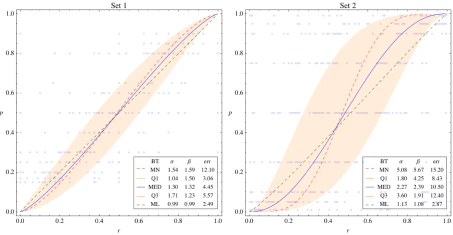
'"$" The quantile regression estimations using densities of r are shown in Figure 6.1. A few observations are in order. The most important is that the median regression for Set 1 is no

longer a straight line as for standard quantile regression, but a slightly S&shaped curve. This is

confirmed by the beta distribution parameters, which are greater than 1 (α = 1.3, β = 1.32).

The range between the lower and upper quantiles is wider than for the standard quantile re&

gression. This may partially be the result of gbt having imperfectly estimated the peaked den&

/ '"!" Quantile regressions based on the densities of r. The gbt densities were used for optimiza& tion. The dashed curves are those obtained using the standard quantile regression estimators.

The results for Set 2 also differ slightly from those obtained using standard regression

estimator. Examining the plots for Set 2 gives the impression that the fit is not the best. The

possibility that the inexactness in the estimation is caused by the functional form of the rela&

tive utility function Q cannot be excluded. This impression, however, also arises from being

accustomed to minimization of the distance expressed in absolute terms of r whereas the

quantile distance does not correspond with this value. The results presented in the boxes show

that the average error is between 3.06 and 5.57 quantiles for Set 1 and between 8.43 and 12.40

quantiles for Set 2, depending on whether lower, median or upper quartile is considered.

0" * 2* 3 4

0"!" The modes of the density functions can be easily calculated using (4.6) or (4.7), and have already been presented in Figures 4.1 and 4.2. The mode regression estimator should

therefore result in r values of the relative utility function which are as close as possible to the

modes of the distributions. One possibility is to proceed similarly as with mean regression and

to use (5.2) with the mean values replaced with the modes. This would result in minimizing

the distances of the estimated curve from the modes. However, a more interesting possibility

is the ratio of the density at the point assumed by the relative utility function to the density at

the mode (where it achieves its maximum). This would produce a function which should be

( )

₍

(

)

₎

1 _mode, ; , ; d M j j d mode d

j _{j j}

d r S d r θ θ θ =

=

∏

(7.1)

where j = 1… M denotes consecutive probabilities pj, d denotes the density function having

parameters d j

θ for probability pj, rj is the value of the relative utility function for this probabil&

ity, and rmode,j denotes the value at the mode for density j.

d mode

S is a function of the relative

utility parameters θ becauser_j =Q−1

(

p_j;θ

)

. As the denominator of (7.1) has no impact on the

maximization procedure, (7.1) may be presented as:

( )

(

)

1

; ,

M

d d

mode j j

j

S θ d r θ

=

=

∏

(7.2)

where the right&hand side may be recognized as the joint probability of observing rj values

given parameters θ. On the other hand, it can also be seen as a function of θ given the densi&

ties d for the respective probabilities. In this way, (7.2) can be recognized as the likelihood of

observing the actual densities of r. Maximizing (7.2) with respect to θ therefore leads to an

estimator of the relative utility function which maximizes the likelihood of observing the

stated densities of r. The mode regression estimator thus appeared to be the maximum likeli&

hood estimator, which is one of the most interesting results of this paper.

0"#"The logarithm of the likelihood function (7.2) yields:

( )

(

)

1

ln ln ; ,

M

d d

j j

j

L

θ

d r

θ

=

=

∑

(7.3)

where Smoded was replaced by d

L . As the density function is described by gbt and the relative

utility function Q by cumulative beta distribution, we obtain:

(

)

(

(

)

)

(

)

(

)

(

)

(

(

)

)

(

)

(

) (

) (

)

1 1 1 1 1 1 1 1

ln , ln ; , ; , ,

1 ln ; , 1 ln 1 ; , ln ,

ln 1 ; , 1 ln .

M d

j j j j

j

M M

j j j j j j

j j

N

j j j j j j

i

L gbt I p

I p I p M B

I p M

α β

α β γ δ λ

γ

α β

δ

α β

γ δ

γ

δ

λ

α β

γ

λ

− = − − = = − = = = − + − − −   − + _ − + +_

∑

∑

∑

∑

(7.4)

0"$" Let Lo denote the maximum value of the likelihood function which can be

achieved as a result of the estimation. The mode can be calculated from (4.6) or from (4.7), so

0 mode, 1

log ln ( ; ).

M

d

j j

j

L d r r

θ

=

=

∑

= (7.5)

The Goodness of Fit measure χ2, which resembles other pseudo&R2 measures, can be given:

2 1 0 log , log e ml L L

χ

= (7.6)

where Le is the maximized likelihood function. The meaning of the measure when presented

in this way, however, is not clear. Bearing in mind that the likelihood function determines

probability, the (geometric) mean ratio of obtained to possible probability (cf. (7.1)) can be

written as:

(

)

(

)

0 0 log log log 1 1 2 2 log

1 mode, 0

; . ; e e L

d _{L L}

M M

j j _{M e M M}

ml d L

j j j M

d r _{L e}

e L d r e θ χ θ − =   _{ }   = =_{ } = =     

∏

 (7.7)

A penalty for the number of parameters of the relative utility function can be introduced:

0 log log 2 3 . e L L M k ml e χ − − = (7.8)

This measure can be expressed as an error:

2 3

1 .

d

ml ml

err = −χ (7.9)

0"%" The results of the estimation are presented in Figure 7.1 along with the values of the distribution modes.

As can be seen, the obtained function is almost linear for both sets of data. These re&

sults confirm the earlier observation achieved using the nonparametric and parametric ap&

proaches and are of great importance. It transpires that the most likely value of the relative

certainty equivalent equals the probability of winning the lottery.

5" +

[image:20.595.72.525.320.555.2]

5"!" Figure 8.1 shows the joint estimation results obtained in Points 5, 6, and 7. This figure can be compared to the results of the nonparametric and parametric regression estima&

tions (Kontek, 2010). In Set 1, the mode regression is almost linear while the median and

mean exhibit some curvature. The graphs for Set 2 are similar. This means that the most likely

lottery valuation is close to its expected value in both cases. Another way of saying this is that

the most likely behavior of the examined groups was fully rational.

/ 5"!" Mean, quantile, and mode regression estimations plotted together.

5"#"This paper concentrated on presenting a regression methodology for inhomogene& ous data encountered in lottery experiments. The paper covered mean, quantile (including

median), and mode (maximum likelihood) regression estimators based on densities of ob&

served variable. The proposed methodology would appear to have several advantages over the

standard procedures. First and foremost, it enables the estimation problems caused by the in&

homogeneity of the data (like heteroskedascicity) to be easily eliminated. Second, the compu&

tational inconveniences of the median and (especially mode) estimators can be eliminated.

Third, it represents errors in a meaningful way (e.g. in terms of quantiles in the quantile re&

mined.

It is not possible to cover all the details and the other subjects related to those already

mentioned in one paper. Some of the subjects touched on require a deeper analysis. These

include other functional forms of density functions especially suited to peaked densities, other

functional forms of the relative utility function, assessing data at the individual level, and es&

timating the relative utility function for multi&prize lotteries. The results presented in this pa&

per should obviously be confirmed for other data sets as well. All this is left for future papers.

5"$" This paper nevertheless proves that inhomogeneity of data has to be taken into ac& count during analysis and evidences the usefulness of the proposed estimation methods. The

proposed methodology seems to have much wider application in econometric research than

just lottery experiments.

!

As stated in 4.6, there appeared to be cases in Set 1 where relative certainty equiva&

lents assumed values of either 0 or 1. This made it impossible to perform the maximum likeli&

hood procedure. In Set 2, relative certainty equivalents which were close to the bounds of the

density function domain distorted the shape of the estimated density curve. These values were

disregarded during the estimation procedure so as to eliminate this problem, but were then

used in further analyses.

If, in a subset of data related to a specific probability, there are k1 data items with a

value of 0, k2 data items with values in the range (0,1), and k3 data items with a value of 1,

then the densities may be defined as follows:

3

1 2

1 , 2 , and 3 ,where 1 2 3 .

k

k k

k k k K

K K K

ρ = ρ = ρ = + + = (A1.1)

The new properties of bt may be given:

(

)

2

2, 3, ; , 3,

m Mean ρ ρ bt r γ δ γ ρ ρ

γ δ

= _ _= +

+ (A1.2)

(

)

(

)

2

(

)

3

2 3

1 1

, , ; , ,

1

m m

var Variance ρ ρ bt r γ δ γ γ δ δ ρ

γ δ

+ − + + +

= _ _=

+ + (A1.3)

(

) (

)

(

)

(

)

2 2

3

1

,

1 1

m r loss

m m

γ δ

γ γ δ δ ρ

− + +

=

gbt properties are as follows:

(

)

2

2, 3, ; , , 3,

m Mean ρ ρ gbt r γ δ λ γ ρ ϕ ρ

γ δ = _ _= + + (A1.5)

(

)

(

)

(

)

(

)

2 3 2

3 2 3

, , ; ,

1 1 1

, 1

var Variance bt r

m m

ρ ρ

γ δ

λ

γ

δ

λ

δ λ ρ

γ ρ

ρ

λ

= _ _ − − _ + + − _+ + + = − (A1.6)

(

) (

)

(

)

(

)

(

)

2 2

3 2 3

1

,

1 1 1

m r loss

m m

λ

λ

γ

δ

λ

δ λ ρ

γ ρ

ρ

− −

=

− − _ + + − _+ + + (A1.7)

which respectively replace (4.3), (4.13) and the loss function inside (5.3).

In the case of the densities based quantile estimator, the quantile qr is calculated as:

(

)

1

1 2 1 1 2

1 2

0 ,

; ,

1 .

d

r j j

if q

q D r if q

if q

ρ

ρ

ρ

θ

ρ

ρ

ρ

ρ

ρ

≤ 



=_ + < < +

 _{≥ +}



(A1.8)

This value is then used in (6.3).

1. Cameron, A. C., Trivedi, P. K., (2005). Microeconometrics. Methods and Applications, Cambridge University Press.

2. Gupta, A. K., Nadarajah, S., (2004), Handbook of Beta Distribution and Its Applications, Marcel Dekker, Inc, New York.

3. Idzikowska, K., (2009). Determinants of the probability weighting function, presented under name Katarzyna Domurat at SPUSM22 Conference, Rovereto, Italy, August 2009, paper Id = 182,

http://discof.unitn.it/spudm22/program_24.jsp .

4. Kontek, K., (2010). Mean, median or Mode? A Striking Conclusion from Lottery Experiments, MPRA Paper http://mpra.ub.uni&muenchen.de/21758/, Available at SSRN:

http://ssrn.com/abstract=1581436

5. Kontek, K., (2009). Lottery Valuation Using the Aspiration / Relative Utility Function, Warsaw School of Economics, Department of Applied Econometrics Working Paper no. 39. Available at SSRN: http://ssrn.com/abstract=1437420 and RePec:wse:wpaper:39.

6. Libby, D. L., Novick, M. R., (1982). Multivariate generalized beta distributions with applications to utility assessment, Journal of Educational Statistics, 7, pp 271&294.

7. Traub, S., Schmidt, U., (2009). An Experimental Investigation of the Disparity between WTA and WTP for Lotteries, Theory & Decision 66 (2009), pp 229&262.