A Matching Method with Panel Data

Munich Personal RePEc Archive

A Matching Method with Panel Data

Nguyen Viet, Cuong

25 April 2010

Online at

https://mpra.ub.uni-muenchen.de/36756/

A Matching Method with Panel Data

Nguyen Viet Cuong1

Abstract

Difference-in-differences with matching is a popular method to measure the impact of an

intervention in health as well as social sciences. This method requires baseline data, i.e.,

data before interventions, which are not always available in reality. Instead, panel data

with two time periods are often collected after interventions begin. In this paper, a simple

matching method is proposed to measure impact of an intervention using two-period

panel data after the intervention.

Keywords: Impact evaluation, difference-in-differences, matching, propensity score,

panel data

JEL classification: H43; C21; J41

1

1. Introduction

Difference-in-differences with matching is a widely-used method to measure impact of

interventions such policies, programs and treatments. However, this method requires

baseline data, i.e., data before interventions, which are not always available for impact

evaluation in reality. Instead, panel data with two time periods are often collected after

interventions begin. When there are panel data without baseline data, one can use

parametric fixed-effect regressions. Compared to matching methods, parametric

regressions have limitation that they must impose functional assumptions on outcome.

The objective of this paper is to discuss identification and estimation of impact of

an intervention using a matching method with two-period panel data after the

intervention. The impact parameter of interest is Average Treatment Effect on the Treated

(ATT).

The paper is structured in four sections. The second section discusses the

matching method using two-period panel data. The third section illustrates this matching

method by an empirical study on impact evaluation of health insurance in Vietnam.

Finally, the fourth section concludes.

2. Matching using Panel Data

The main objective of impact evaluation of an intervention is to assess the extent to

which the intervention has changed outcome of subjects. To make definition explicit,

suppose that there is an intervention of interest, and denote by D the binary variable of

participation in the intervention, i.e. D=1 if one participates in the intervention, and

0

=

D otherwise. Let Y denote observed outcome. This variable can receive two values

depending on D: Y =Y1 if D=1, and Y =Y0 if D=0. The most popular parameter in

impact evaluation is ATT,which is defined as (Heckman et al., 1999):2

) 1 (

) 1

( ₁ = − ₀ =

=E Y D E Y D

ATT . (1)

One can be interested in ATT conditional on observed variables X:

( )=E(Y1|X,D=1)−E(Y0|X,D=1)

ATT_X . (2)

In (2), E(Y₀|X,D=1) which is the expected conditional outcome of the

participants had they not received the intervention is not observed. Thus, estimation of

) (X

ATT is not straightforward. The following sections discuss how to estimate ATT₍X₎ and

ATT using matching methods with panel data.

2.2. Difference-in-differences with Matching

When panel data on participants and non-participants before and after an intervention are

available, ATT can be estimated using a method of difference-in-differences with

matching. The basic idea of matching is to find a control group that has similar

2

distribution of X as the treatment group.3 Matching is combined with

difference-in-difference estimation to allow intervention selection to be based on unobserved variables.

However, this method requires the unobserved variables be time-invariant.

Let Y0F denote pre-intervention outcome. After the intervention, let Y1S and Y0S

denote potential outcomes in states of intervention and no-intervention, respectively.4

(X)

ATT after the intervention is defined as:

) |X, D ) - E(Y |X, D

E(Y

ATT_(X) = _1S =1 _0S =1 (3)

The difference-in-differences with matching method relies on an assumption that

conditional on X, difference in outcome expectations between the participants and

non-participants is time-invariant:

) 0 , | ( ) 1 , | ( ) 0 , | ( ) 1 , |

(Y₀ X D= −E Y₀ X D= =E Y₀ X D= −E Y₀ X D=

E _{F F S S} . (4)

Then, ATT(X) can be identified, since:

[

]

[

]

[

] [

]

) |X,D E(Y ) |X,D E(Y ) |X,D E(Y ) |X,D E(Y )- |X, D ) - E(Y |X, D E(Y ATT F F S S S S F F S S (X) 0 1 0 1 0 1 0 1 1 1 0 0 0 1 0 0 0 0 0 1 = − = = = = = − = + = − = = = = (5)

ATT is also identified, since:

= = = 1 1 X|D (X) ) dF(X|D ATT

ATT . (6)

The matching estimator is based on equation (5). It is equal to difference in

differences in outcomes between the treatment and control groups before and after the

intervention.

3

There is large literature on matching methods, e.g., Rubin (1979), Rosenbaum and Rubin (1983), and Smith and Todd (2005).

4

2.3. Matching using Panel Data without Baseline Data

In reality, baseline data are not always available for intervention evaluation. Instead,

panel data with two time periods are often collected after the intervention begins. An

intervention can take place continuously. There can be not only people leaving but also

ones newly entering the intervention. Assume that there are two time periods, and let D1

and D2 denote the binary variables of the intervention status in the first and second

periods, respectively. In the first period, let Y1F and Y0F denote potential outcomes with

and without the intervention, respectively. Further, let Y1S and Y0S denote the potential

outcomes with and without the intervention in the second period, respectively. Suppose

that we are interested in ATT(X) in the second period, which is expressed as follows:

) 1 , | ( ) 1 , |

( _{1 2 0 2}

)

( =E Y X D = −E Y X D =

ATTS_{X S S} . (7)

Note that we cannot observe E(Y0S | X,D2 =1). The single matching method assumes

that: ) 0 , | ( ) 1 , |

(Y0 X D2 = =EY0 X D2 =

E _{S S} , (8)

which eliminates any correlation between the intervention and unobserved variables

affecting the outcomes. Using panel data, we can identify the intervention impact without

the assumption specified by (8). Rewrite (7) as follows:

[

]

[

]

) 1 , | 0 Pr( ) 1 , 1 , | ( ) 1 , 1 , | ( ) 1 , | 1 Pr( 2 1 0 2 1 1 2 1 2 1 0 2 1 1 2 1 ) ( = = − = = = = + = = − = = = = = D D X Y E D D X Y E D X D D D X Y E D D X Y E D X D ATT S S S S S X (9)

[

]

[

]

) 0 , 0 , | ( ) 1 , 0 , | ( 2 1 0 2 1 0 2 1 0 2 1 0 = = − = = = = = − = = D D X Y E D D X Y E D D X Y E D D X Y E F F S S (10)

[

]

[

]

) 1 , 1 , | ( ) 1 , 1 , | ( 2 1 1 2 1 0 2 1 1 2 1 0 = = − = = = = = − = = D D X Y E D D X Y E D D X Y E D D X Y E F S F S (11)

The first assumption means that difference in the no-intervention outcome (conditional on

X) between people who do not participate in the intervention in both periods and those

who participate in the intervention only in the second period is unchanged overtime. This

assumption is similar to the assumption of the method of difference-in-differences with

matching. The second assumption means that difference between the no-intervention

outcome in the second period and the intervention outcome in the first period is the same

for people who participate in the intervention in both periods and those who participate in

the intervention in the first period but not in the second one.

Substitute (10) and (11) into (9) and rewrite (9) as follows:

[

]

{

[

]}

[

]

{

[

]}

) 0 , 0 , | ( ) 1 , 0 , | ( ) 1 , | 0 Pr( ) 0 , 1 , | ( ) 1 , 1 , | ( ) 0 , 1 , | ( ) 1 , 1 , | ( ) 1 , | 1 Pr( 2 1 0 2 1 0 2 1 0 2 1 1 2 1 2 1 1 2 1 1 2 1 0 2 1 1 2 1 ) ( = = − = = = = − = = = = + = = − = = = = − = = = = = D D X Y E D D X Y E D D X Y E D D X Y E D X D D D X Y E D D X Y E D D X Y E D D X Y E D X D ATT F F S S F F S S S X (12)

Now, S X

ATT_{( )}is identified since all terms in (12) can be observed. The unconditional

parameter is also identified by (6). Matching can be performed according to (12): (i)

people who participate in the intervention in both periods are matched with those who

participate in the intervention only in the first period, (ii) people who participate in the

intervention only in the second period are matched with those who do not participate in

To find the control groups who have similar variables X, we requires common

support assumptions as follows:

1 ) 1 , | 1 (

0<P D₂= X D₁= < (13)

1 ) 0 , | 1 (

0<P D₂= X D₁= < (14)

These assumptions mean that given the intervention status in the first period there are

non-participants who have the X variables similar to those of the participants in the

second period.

A problem is how to match non-participants with participants. Since a paper by

Rosenbaum and Rubin (1983), the matching is often conducted based on the probability

of being assigned into the intervention, which is called the propensity score.5 In our case,

the propensity score is the probability of participating in the intervention in the second

period given variables X and D1. We can use logit or probit regressions to predict

) | 1 ( ˆ

2 X

D

P = in the separate samples of people with D₁=1 and D₁=0.

After the treatment and control groups are constructed, ATT can be estimated by

differences in outcomes between the treatment and control groups as specified by (12).

The standard errors are calculated using bootstrap techniques.

Finally, one can be interested in ATT_(X)for the first period:

) 1 , | ( ) 1 , |

( _{1 1 0 1}

)

( =E Y X D = −E Y X D =

ATTF_{X F F} . (15)

which is estimated very similarly by reversing the first and second periods in the

estimation of S X ATT_{( )}.

5

3. Empirical Example

This section illustrates estimation of impact of health insurance on the number of annual

healthcare contacts in Vietnam using the matching method. In Vietnam, health insurance

has been implemented since 1992, and there are no baseline data for health insurance. To

measure impacts of health insurance, the paper uses data from Vietnam Household Living

Standard Surveys (VHLSS) in 2004 and 2006. These surveys were conducted by General

Statistical Office of Vietnam. These surveys set up panel data, which are representative

for national, rural and urban levels. The number of individuals in the panel data used is

16685.

Table 1 presents the distribution of sample individuals in the panel data of the

surveys by health insurance. Not all Vietnamese people were covered by health

insurance. There were 4802 and 6337 people having health insurance in 2004 and 2006,

respectively. There were 3401 people having health insurance in both 2004 and 2006.

Table 1: Distribution of sampled individuals by health insurance

Uninsured in 2004

Insured in 2004 Total

Uninsured in 2006 8947 1401 10348

Insured in 2006 2936 3401 6337

Total 11883 4802 16685

Source: Estimation from panel data of VHLSS 2004-2006.

To estimate the intervention impact, we construct two treatment groups and two

control groups. The first treatment group includes people having health insurance in both

2004 and 2006. This group is matched with a control group who include people having

health insurance in 2004 but not 2006. The second treatment group are those who are

uninsured in both 2004 and 2006. The treatment and control groups are matched based on

the closeness of the propensity score. The propensity score are the probability of being

insured in 2006, which are estimated from two logit regressions: the first using the

sample of people insured in 2004, and the second using the sample of people uninsured in

2004. Control variables in the logit regressions include per capita income in 2004 and

2006, age in 2004, sickness in 2004 and 2006, educational degree in 2004, regional

dummy variables, and urbanity. Once the treatment and control groups are setup, the

intervention impacts can be estimated by differences in outcome between the treatment

and control groups overtime (see equation (12)).

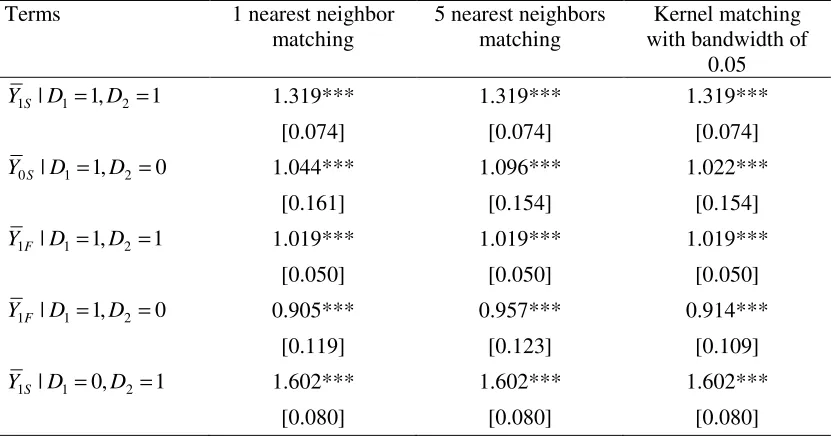
Table 2 presents impact estimates of health insurance on the number of annual

healthcare contacts of the insured people in 2006. It presents all the estimates which are

used to compute ATT. All the three matching estimators give similar results. The impact

estimates of ATT are statistically significant at 10%. Health insurance helped the insured

people increase the number of annual healthcare contacts by around 0.17 in 2006.

Table 2: Impacts of Health Insurance

Terms 1 nearest neighbor matching

5 nearest neighbors matching

Kernel matching with bandwidth of

0.05 1

, 1

| _{1 2}

1 D = D =

Y_S 1.319*** 1.319*** 1.319***

[0.074] [0.074] [0.074]

0 , 1

| _{1 2}

0 D = D =

Y_S 1.044*** 1.096*** 1.022***

[0.161] [0.154] [0.154]

1 , 1

| _{1 2}

1 D = D =

Y_F 1.019*** 1.019*** 1.019***

[0.050] [0.050] [0.050]

0 , 1

| _{1 2}

1 D = D =

Y_F 0.905*** 0.957*** 0.914***

[0.119] [0.123] [0.109]

1 , 0

| _{1 2}

1 D = D =

Y_S 1.602*** 1.602*** 1.602***

Terms 1 nearest neighbor matching

5 nearest neighbors matching

Kernel matching with bandwidth of

0.05 0

, 0

| _{1 2}

0 D = D =

Y_S 1.231*** 1.227*** 1.229***

[0.095] [0.103] [0.112]

1 , 0

| _{1 2}

0 D = D =

Y_F 1.251*** 1.251*** 1.251***

[0.083] [0.083] [0.083]

0 , 0

| _{1 2}

0 D = D =

Y_F 1.054*** 1.087*** 1.068***

[0.098] [0.096] [0.094]

1 ˆ_T T

A 0.161* 0.160* 0.191*

[0.095] [0.091] [0.110]

0 ˆ_T T

A 0.173* 0.211* 0.190*

[0.108] [0.123] [0.119]

) 1 | 1

Pr(D₁= D₂ = 0.537*** 0.537*** 0.537***

[0.010] [0.010] [0.010]

T T

Aˆ 0.166* 0.184* 0.190*

0.097 [0.108] [0.113]

Note:

[

] [

]

ˆ

2 1 1 2

1 1 2

1 0 2

1 1

1= Y D = D = − Y D = D = - Y D = D = − Y D = D =

T T

A _{S S F F}

[

] [

]

2 1 0 2

1 0 2

1 0 2

1 1

0= Y D = D = − Y D = D = - Y D = D = − Y D = D =

T T

A _{S S F F}

0 2

1 1

2

1 1| 1) ˆ Pr( 0| 1) ˆ

Pr(

ˆ_{T D D ATT D D ATT}

T

A = = = + = =

Figures in brackets are standard errors, which are corrected for sampling weights and estimated using non-parametric bootstrap with 500 replications.

* significant at 10%; ** significant at 5%; *** significant at 1% Source: Estimation from panel data of VHLSS 2004-2006.

4. Conclusion

In impact evaluation of an intervention, baseline data are not always available. Thus, the

method of difference-in-differences with matching cannot be applied straightforward.

Two-period panel data can be collected after interventions start. This paper discusses the

identification and estimation of ATT using the matching with two-period panel data. It is

be measured as a weighted average of intervention impacts on groups with different

intervention statuses in the two periods.

References

Heckman, J., R. Lalonde and J. Smith, 1999. The Economics and Econometrics of Active

Labor Market Programs. Handbook of Labor Economics, Volume 3, Ashenfelter, A. and

D. Card, eds., Elsevier Science.

Rosenbaum, P. and R. Rubin, 1983. The Central Role of the Propensity Score in

Observational Studies for Causal Effects. Biometrika 70 (1), 41-55.

Rubin, D., 1979. Using Multivariate Sampling and Regression Adjustment to Control

Bias in Observational Studies. Journal of the American Statistical Association. 74, 318–

328.

Smith, J. and P. Todd, 2005. Does Matching Overcome LaLonde’s Critique of