Newton-Stein Method:
An Optimization Method for GLMs via Stein’s Lemma
Murat A. Erdogdu [email protected]
Department of Statistics Stanford University
Stanford, CA 94305-4065, USA
Editor:Qiang Liu
Abstract
We consider the problem of efficiently computing the maximum likelihood estimator in
Generalized Linear Models (GLMs) when the number of observations is much larger than the number of coefficients (n p 1). In this regime, optimization algorithms can immensely benefit from approximate second order information. We propose an alternative way of constructing the curvature information by formulating it as an estimation problem and applying aStein-type lemma, which allows further improvements through sub-sampling and eigenvalue thresholding. Our algorithm enjoys fast convergence rates, resembling that of second order methods, with modest per-iteration cost. We provide its convergence analysis for the general case where the rows of the design matrix are samples from a sub-Gaussian distribution. We show that the convergence has two phases, a quadratic phase followed by a linear phase. Finally, we empirically demonstrate that our algorithm achieves the highest performance compared to various optimization algorithms on several data sets.
Keywords: Optimization, Generalized Linear Models, Newton’s method, Sub-sampling
1. Introduction
Generalized Linear Models (GLMs) play a crucial role in numerous statistical and machine learning problems. GLMs formulate the natural parameter in exponential families as a linear model and provide a miscellaneous framework for statistical methodology and supervised learning tasks. Celebrated examples include linear, logistic, multinomial regressions and applications to graphical models (Nelder and Baker, 1972; McCullagh and Nelder, 1989; Koller and Friedman, 2009).
In this paper, we focus on how to solve the maximum likelihood problem efficiently in the GLM setting when the number of observations n is much larger than the dimension of the coefficient vector p, i.e., n p 1. GLM optimization task is typically expressed as a minimization problem where the objective function is the negative log-likelihood that is denoted by `(β) where β ∈ Rp is the coefficient vector. Many optimization algorithms
are available for such minimization problems (Bishop, 1995; Boyd and Vandenberghe, 2004; Nesterov, 2004). However, only a few uses the special structure of GLMs. In this paper, we consider updates that are specifically designed for GLMs, which are of the from
β ←β−γQ∇β`(β), (1)
For the updates of the form Equation 1, the performance of the algorithm is mainly determined by the scaling matrixQ. ClassicalNewton’s method andnatural gradient descent
can be recovered by simply taking Q to be the inverse Hessian and the inverse Fisher’s information at the current iterate, respectively (Amari, 1998; Nesterov, 2004). Second order methods may achieve quadratic convergence rate, yet they suffer from excessive cost of computing the scaling matrix at every iteration. On the other hand, if we takeQto be the identity matrix, we recover the standard gradient descent which has a linear convergence rate. Although the convergence rate of gradient descent is considered slow compared to that of second order methods such as Newton’s method, modest per-iteration cost makes it practical for large-scale optimization.
The trade-off between convergence rate and per-iteration cost has been extensively stud-ied (Bishop, 1995; Boyd and Vandenberghe, 2004; Nesterov, 2004). In np 1 regime, the main objective is to construct a scaling matrix Qthat is computational feasible which also provides sufficient curvature information. For this purpose, several Quasi-Newton meth-ods have been proposed (Bishop, 1995; Nesterov, 2004). Updates given by Quasi-Newton methods satisfy an equation which is often called theQuasi-Newton relation. A well-known member of this class of algorithms is theBroyden-Fletcher-Goldfarb-Shanno (BFGS) algo-rithm (Broyden, 1970; Fletcher, 1970; Goldfarb, 1970; Shanno, 1970).
In this paper, we propose a Newton-type algorithm that utilizes the special structure of GLMs by relying on a Stein-type lemma (Stein, 1981). It attains fast convergence rates with low per-iteration cost. We call our algorithmNewton-Stein method which we abbreviate as
NewSt. Our contributions can be summarized as follows:
• We recast the problem of constructing a scaling matrix as an estimation problem and apply a Stein-type lemma along with the sub-sampling technique to form a computa-tionally feasibleQ.
• Newton-Stein method allows further improvements through eigenvalue shrinkage, eigen-value thresholding, sub-sampling and various other techniques that are available for covariance estimation.
• Excessive per-iteration cost ofO(np2+p3) of Newton’s method is replaced byO(np+
p2) per-iteration cost and a one-time O(|S|p2) cost, where|S|is the sub-sample size. • Assuming that the rows of the design matrix are i.i.d. and have bounded support (or sub-Gaussian), and denoting the iterates of Newton-Stein method by {βˆt}t, we prove
a bound of the form
βˆt+1−β∗
2 ≤τ1
βˆt−β∗
2+τ2
βˆt−β∗
2
2, (2)
whereβ∗ is the true minimizer andτ1,τ2 are the convergence coefficients. The above bound implies that the local convergence starts with a quadratic phase and transitions into linear as the iterate gets closer to the true minimizer. We further establish a global convergence result of Newton-Stein method coupled with a line search algorithm.
The rest of the paper is organized as follows: Section 1.1 surveys the related work and Section 1.2 introduces the notations we use throughout the paper. Section 2 briefly discusses the GLM framework and its relevant properties. In Section 3, we introduce Newton-Stein method, develop its intuition, and discuss the computational aspects. Section 4 covers the theoretical results and in Section 4.4 we discuss how to choose the algorithm parameters. Section 5 provides the empirical results where we compare the proposed algo-rithm with several other methods on four data sets. Finally, in Section 6, we conclude with a brief discussion along with a few future research directions.
1.1 Related Work
There are numerous optimization techniques that can be used to find the maximum like-lihood estimator in GLMs. For moderate values of n and p, the classical second order methods such as Newton’s method (also referred to as Newton-Raphson) are commonly used. In large-scale problems, data dimensionality is the main factor while determining the optimization method, which typically falls into one of two major categories: online and batch methods. Online methods use a gradient (or sub-gradient) of a single, randomly selected observation to update the current iterate (Robbins and Monro, 1951). Their per-iteration cost is independent ofn, but the convergence rate might be extremely slow. There are several extensions of the classical stochastic descent algorithms, providing significant improvement and improved stability (Bottou, 2010; Duchi et al., 2011; Schmidt et al., 2013; Kolte et al., 2015).
On the other hand, batch algorithms enjoy faster convergence rates, though their per-iteration cost may be prohibitive. In particular, second order methods enjoy quadratic convergence, but constructing the Hessian matrix generally requires excessive amount of computation. To remedy this issue, most research is focused on designing an approximate and cost-efficient scaling matrix. This idea lies at the core of Quasi-Newton methods such as BFGS (Bishop, 1995; Nesterov, 2004).
Another approach to construct an approximate Hessian makes use of sub-sampling tech-niques (Martens, 2010; Byrd et al., 2011; Vinyals and Povey, 2011; Erdogdu and Montanari, 2015; Roosta-Khorasani and Mahoney, 2016a,b). Many contemporary learning methods rely on sub-sampling as it is simple and it provides significant boost over the first order meth-ods. Further improvements through conjugate gradient methods and Krylov sub-spaces are available. Sub-sampling can also be used to obtain an approximate solution, with certain large deviation guarantees (Dhillon et al., 2013).
There are many composite variants of the aforementioned methods, that mostly com-bine two or more techniques. Well-known composite algorithms are the combinations of sub-sampling and Quasi-Newton (Schraudolph et al., 2007; Byrd et al., 2016), stochastic and deterministic gradient descent (Friedlander and Schmidt, 2012), natural gradient and Newton’s method (Le Roux and Fitzgibbon, 2010), natural gradient and low-rank approx-imation (Le Roux et al., 2008), sub-sampling and eigenvalue thresholding (Erdogdu and Montanari, 2015).
1.2 Notation
Let [n] ={1,2, ..., n} and denote by |S|, the size of a setS. The gradient and the Hessian of f with respect to β are denoted by ∇βf and ∇2
βf, respectively. The j-th derivative of
a function f(w) is denoted by f(j)(w). For a vector x and a symmetric matrix X, kxk 2 and kXk2 denote the `2 and spectral norms of x and X, respectively. kxkψ2 denotes the sub-Gaussian norm, which will be defined later. Sp−1 denotes the p-dimensional sphere. PC denotes the projections onto the setC, and Bp(R)⊂Rp denotes the p-dimensional ball of radius R. For a random variable x and density f, x ∼ f means that the distribution of x follows the density f. Multivariate Gaussian density with mean µ ∈ Rp and
covari-ance Σ ∈ Rp×p is denoted as N
p(µ,Σ). For random variables x, y, d(x, y) and D(x, y)
denote probability metrics (will be explicitly defined) measuring the distance between the distributions ofx and y. N[](· · ·) andT denote the bracketing number and -net.
2. Generalized Linear Models
Distribution of a random variable y ∈ R belongs to an exponential family with natural parameterη ∈Rif its density can be written as
f(y|η) =eηy−φ(η)h(y),
where φis the cumulant generating function and h is the carrier density. Let y1, y2, ..., yn
be independent observations such that ∀i∈ [n], yi ∼ f(yi|ηi). Denoting η = (η1, ..., ηn)T,
the joint likelihood can be written as
f(y1, y2, ..., yn|η) = exp ( n
X
i=1
[yiηi−φ(ηi)]
) n
Y
i=1
h(yi). (3)
We consider the problem of learning the maximum likelihood estimator in the above expo-nential family framework, where the vector η∈Rn is modeled through the linear relation,
η =Xβ,
for some design matrix X ∈ Rn×p with rows xi ∈ Rp, and a coefficient vector β ∈ Rp. This formulation is known asGeneralized Linear Models (GLMs) with canonical links. The cumulant generating functionφdetermines the class of GLMs, i.e., for ordinary least squares (OLS)φ(z) =z2/2, for logistic regression (LR)φ(z) = log(1+ez), and for Poisson regression (PR)φ(z) =ez.
Finding the maximum likelihood estimator in the above formulation is equivalent to minimizing the negative log-likelihood function`(β),
`(β) = 1
n
n X
i=1
[φ(hxi, βi)−yihxi, βi], (4)
and the Hessian of`(β) can be written as:
∇β`(β) = 1
n
n X
i=1
h
φ(1)(hxi, βi)xi−yixi i
, ∇2
β`(β) =
1
n
n X
i=1
φ(2)(hxi, βi)xixTi . (5)
For a sequence of scaling matrices {Qt}t>0 ∈Rp×p, we consider iterations of the form
ˆ
βt+1 = ˆβt−γtQt∇β`( ˆβt)
where γt is the step size. The above iteration is our main focus, but with a new approach
on how to compute the sequence of matrices {Qt}t>0. We will formulate the problem of finding a scalableQtas an estimation problem and apply a Stein-type lemma that provides us with a computationally efficient update rule.
3. Newton-Stein Method
Classical Newton-Raphson (or simply Newton’s) method is the standard approach for train-ing GLMs for moderately large date sets. However, its per-iteration cost makes it imprac-tical for large-scale optimization. The main bottleneck is the computation of the Hessian matrix that requiresO(np2) flops which is prohibitive whennp1. Numerous methods have been proposed to achieve the fast convergence rate of Newton’s method while keeping the per-iteration cost manageable. To this end, a popular approach is to construct a scaling matrixQt, which approximates the inverse Hessian at every iterationt.
The task of constructing an approximate Hessian can be viewed as an estimation prob-lem. Assuming that the rows of X are i.i.d. random vectors, the Hessian of the negative log-likelihood of GLMs with a cumulant generating function φ has the following sample average form
Qt−1= 1
n
n X
i=1
xixTi φ(2)(hxi, βi)≈E[xxTφ(2)(hx, βi)].
We observe that
Qt−1
is just a sum of i.i.d. matrices. Hence, the true Hessian is nothing but a sample mean estimator to its expectation. Another natural estimator would be the sub-sampled Hessian method which is extensively studied by Martens, 2010; Byrd et al., 2011; Erdogdu and Montanari, 2015; Roosta-Khorasani and Mahoney, 2016a. Therefore, our goal is to propose an estimator for the population level Hessian that is also computationally efficient. Since nis large, the proposed estimator will be close to the true Hessian.
We use the following Stein-type lemma to find a more efficient estimator to the expec-tation of the Hessian.
Lemma 1 (Stein-type lemma) Assume that x ∼ Np(0,Σ) and β ∈ Rp is a constant
vector. Then for any function f :R→R that is twice “weakly”differentiable, we have
ExxTf(hx, βi)=E[f(hx, βi)]Σ+E
h
Algorithm 1 Newton-Stein Method Input: βˆ0,|S|, ,{γt}t≥0.
1. Estimate the covariance using a random sub-sample S ⊂[n]:
b
ΣS = |S1|Pi∈SxixTi.
2. while βˆt+1−βˆt
2 > do ˆ
µ2( ˆβt) = n1 Pni=1φ(2)(hxi,βˆti), µˆ4( ˆβt) = n1Pni=1φ(4)(hxi,βˆti),
Qt= 1 ˆ
µ2( ˆβt)
"
b
Σ−S1−
ˆ
βt[ ˆβt]T ˆ
µ2( ˆβt)/µˆ4( ˆβt) +hΣbSβˆt,βˆti #
,
ˆ
βt+1 = ˆβt−γtQt∇β`( ˆβt),
t←t+ 1.
3. end while Output: βˆt.
identityxg(x|Σ)dx=−Σdg(x|Σ) and write
E[xxTf(hx, βi)] =
Z
xxTf(hx, βi)g(x)dx,
=Σ
Z
f(hx, βi)g(x|Σ)dx+
Z
βxTf(1)(hx, βi)g(x|Σ)dx
,
=Σ
E[f(hx, βi)] +
Z
ββTf(2)(hx, βi)g(x|Σ)dxΣ
,
=E[f(hx, βi)]Σ+E
h
f(2)(hx, βi)iΣββTΣ.
The right hand side of Equation 6 is a rank-1 update to the first term. Hence, its inverse can be computed with O(p2) cost. Quantities that change at each iteration are the ones that depend onβ, i.e.,
µ2(β) =E[φ(2)(hx, βi)], and µ4(β) =E[φ(4)(hx, βi)].
Note that µ2(β) and µ4(β) are scalar quantities and they can be estimated by their cor-responding sample means ˆµ2(β) and ˆµ4(β) (explicitly defined at Step 2 of Algorithm 1) respectively, with only O(np) computation.
To complete the estimation task suggested by Equation 6, we need an estimator for the covariance matrix Σ. A natural estimator is the sample mean where, we only use a sub-sample of the indices S ⊂ [n] so that the cost is reduced to O(|S|p2) from O(np2). Sub-sampling based sample mean estimator is denoted by ΣbS = |S1|
P
−4 −3 −2 −1 0
0 100 200 300 400
Dimension (p)
lo
g10
(
Estimation error
)
Randomness Bernoulli Gaussian Poisson Uniform Difference between estimated and true Hessian
−3 −2 −1 0
0 10 20 30 40 50
Iterations
lo
g10
(
E
rr
o
r
)
Sub−sample size NewSt:S=1000 NewSt:S=10000 Convergence Rate
Figure 1: The left plot demonstrates the accuracy of proposed Hessian estimation over different distributions. Number of observations is set to be n = O(plog(p)). The right plot shows the phase transition in the convergence rate of Newton-Stein method (NewSt ). Convergence starts with a quadratic rate and transitions into linear. Plots are obtained usingCovertype data set.
widely used in large-scale problems (Vershynin, 2010). We highlight the fact that Lemma 1 replacesO(np2) per-iteration cost of Newton’s method with a one-time cost ofO(np2). We further use sub-sampling to reduce this one-time cost toO(|S|p2), and obtain the following Hessian estimator at β
Qt−1
| {z }
∈Rp×p
= ˆµ2(β)
| {z }
∈R
b
ΣS |{z}
∈Rp×p
+ ˆµ4(β)
| {z }
∈R
rank-1 update
z }| {
b
ΣSββTΣbS
| {z }
∈Rp×p
(7)
We emphasize that any covariance estimation method can be applied in the first step of the algorithm. There are various estimation techniques most of which rely on the concept of shrinkage (Cai et al., 2010; Donoho et al., 2013). This is because, important curvature information is generally contained in the largest few spectral features (Erdogdu and Monta-nari, 2015). In particular, for a given thresholdr, we suggest to use the largestreigenvalues of the sub-sampled covariance estimator ΣbS, and setting rest of them to (r+ 1)-th
eigen-value. This operation helps denoising and provides additional computational benefits when inverting the covariance estimator (Erdogdu and Montanari, 2015).
Inverting the constructed Hessian estimator can make use of the low-rank structure. First, notice that the updates in Equation 7 are based on rank-1 matrix additions. Hence, we can simply apply Sherman–Morrison inversion formula to Equation 7 and obtain an explicit equation for the scaling matrixQt(Step 2 of Algorithm 1). This formulation would impose another inverse operation on the covariance estimator. We emphasize that this operation is performed once. Therefore, instead ofO(p3) per-iteration cost of Newton’s method due to inversion, Newton-Stein method (NewSt) requiresO(p2) per-iteration and a one-time cost of O(p3). Assuming that Newton-Stein and Newton methods converge inT1 andT2 iterations respectively, the overall complexity of Newton-Stein is O npT1+p2T1+ (|S|+p)p2
O npT1+p2T1+|S|p2
whereas that of Newton is O(np2T2+p3T2). We show both em-pirically and theoretically that the quantitiesT1 and T2 are close to each other.
The convergence rate of Newton-Stein method has two phases. Convergence starts quadratically and transitions into linear rate when it gets close to the true minimizer. The phase transition behavior can be observed through the right plot in Figure 1. This is a consequence of the bound provided in Equation 2, which is the main result of our theorems on the local convergence (given in Section 4).
Even though Lemma 1 assumes that the covariates are multivariate Gaussian random vectors, in Section 4, the only assumption we make on the covariates is either bounded support or sub-Gaussianity, both of which cover a wide class of random variables including Bernoulli, elliptical distributions, bounded variables etc. The left plot of Figure 1 shows that the estimation is accurate for many distributions. This is a consequence of the fact that the proposed estimator in Equation 7 relies on the distribution ofxonly through inner products of the form hx, vi, which in turn results in an approximate normal distribution due to the central limit theorem. To provide more intuition, we explain this through zero-biased transformationswhich is a general version of Stein’s lemma for arbitrary distributions (Goldstein and Reinert, 1997).
Definition 2 Let z be a random variable with mean 0 and varianceσ2. Then, there exists a random variable z∗ that satisfiesE[zf(z)] =σ2E[f(1)(z∗)], for all differentiable functions
f. The distribution of z∗ is said to be the z-zero-bias distribution.
The normal distribution is the unique distribution whose zero-bias transformation is itself (i.e. the normal distribution is a fixed point of the operation mapping the distribution of z
to that ofz∗). The distribution ofz∗ is referred to asz-zero-bias distribution and is entirely determined by the distribution ofz. Properties such as existence can be found, for example, in Chen et al., 2010.
To provide some intuition behind the usefulness of Lemma 1 even for arbitrary distri-butions, we use zero-bias transformations. For simplicity, assume that the covariate vector
x has i.i.d. entries from an arbitrary distribution with mean 0, and variance 1. Then the zero-bias transformation applied twice to the entry (i, j) of matrix E[xxTf(hx, βi)] yields
E[xixjf(hx, βi)] =
E[f(βix∗i + Σk6=ixkβk)] +βi2E
f(2)(βix∗∗i + Σk6=ixkβk)
if i=j,
βiβjEf(2)(βix∗i +βjx∗j+ Σk6=i,jxkβk)
if i6=j,
where x∗i and x∗∗i have xi-zero-bias and x∗i-zero-bias distributions, respectively. For each
entry (i, j) at most two summands ofhx, βi= Σkxkβkchange their distributions. Therefore,
if β is well spread andp is sufficiently large, the sums inside the expectations will behave similar to the inner product hx, βi. Correspondingly, the above equations will be close to their Gaussian counterpart as given in Equation 6.
4. Theoretical Results
4.1 Preliminaries
Hessian estimation described in the previous section relies on a Gaussian approximation. For theoretical purposes, we use the following probability metric to quantify the gap between the distribution ofxi’s and that of a normal vector.
Definition 3 Given a family of functions H, and random vectorsx, y∈Rp, forHand any
h∈ H, define
dH(x, y) = sup
h∈H
dh(x, y) where dh(x, y) =
E[h(x)]−E[h(y)] .
Many probability metrics can be expressed as above by choosing a suitable function class H. Examples include Total Variation (TV), Kolmogorov and Wasserstein metrics (Gibbs and Su, 2002; Chen et al., 2010). Based on the second and the fourth derivatives of the cumulant generating function, we define the following function classes:
H1=nh(x) =φ(2)(hx, βi) :β ∈ Co, H2=nh(x) =φ(4)(hx, βi) :β ∈ Co,
H3 =
n
h(x) =hv, xi2φ(2)(hx, βi) :β ∈ C,kvk2= 1
o
,
where C ∈ Rp is a closed, convex set that is bounded by the radius R. Exact calculation
of such probability metrics are often difficult. The general approach is to upper bound the distance by a more intuitive metric. In our case, we observe that dHj(x, y) for j = 1,2,3,
can be easily upper bounded by dTV(x, y) up to a scaling constant, when the covariates have bounded support.
In our theoretical results, we rely on projected updates onto a closed convex setC, which are of the form
ˆ
βt+1 =Pt
C
ˆ
βt−γQt∇β`( ˆβt) where the projection is defined as Pt
C(β) = argminw∈C12kw−βk2Qt−1, with C bounded by R. This is a special case of proximal Newton-type algorithms and further generalization is straightforward (See Lee et al., 2014). We will further assume that the covariance matrix has full rank and its smallest eigenvalue is lower bounded by a positive constant.
4.2 Bounded Covariates
We have the following per-step bound for the iterates generated by the Newton-Stein method, when the covariates are supported on a ball.
Theorem 4 (Local convergence) Assume that the covariatesx1, x2, ..., xnare i.i.d.
ran-dom vectors supported on a ball of radius √K with
E[xi] = 0 and ExixTi
=Σ.
Further assume that the cumulant generating function φ has bounded 2nd-5th derivatives and that the set C is bounded by R. For βˆt t>0 given by the Newton-Stein method for γ = 1, define the event
E=
inf kuk2=1
µ2( ˆβ
t)hu,Σui+µ4( ˆβt)hu,Σβˆti2 >2κ
−1 ∀t, β ∗ ∈ C
for some positive constantκ, and the optimal value β∗. Ifn,|S|and pare sufficiently large,
then there exist constantsc, c1, c2 depending on the radiiK, R, P(E) and the bounds onφ(2)
and |φ(4)|such that conditioned on the event E, with probability at least 1−c/p2, we have
βˆt+1−β∗
2 ≤τ1
βˆt−β∗
2+τ2
βˆt−β∗
2
2, (9)
where the coefficients τ1 and τ2 are deterministic constants defined as
τ1 =κD(x, z) +c1κ
r p
min{p/log(p)|S|, n/log(n)}, τ2=c2κ, (10)
and D(x, z) is defined as
D(x, z) =kΣk2 dH1(x, z) +kΣk 2
2R2 dH2(x, z) +dH3(x, z), (11)
for a multivariate Gaussian random variablez with the same mean and covariance as xi’s.
The bound in Equation 9 holds with high probability, and the coefficients τ1 and τ2 are deterministic constants which will describe the convergence behavior of the Newton-Stein method. Observe that the coefficientτ1 is sum of two terms: D(x, z) measures how accurate the Hessian estimation is, and the second term depends on the sub-sampling size |S| and the data dimensionsn, p.
Theorem 4 shows that the convergence of Newton-Stein method can be upper bounded by a compositely converging sequence, that is, the squared term will dominate at first pro-viding us with a quadratic rate, then the convergence will transition into a linear phase as the iterate gets close to the optimal value. The coefficientsτ1 andτ2 govern the linear and quadratic terms, respectively. The effect of sub-sampling appears in the coefficient of linear term. In theory, there is a threshold for the sub-sampling size|S|, namelyO(n/log(n)), be-yond which further sub-sampling has no effect. The transition point between the quadratic and the linear phases is determined by the sub-sampling size and the properties of the data. The phase transition behavior can be observed through the right plot in Figure 1.
Using the above theorem, we state the following corollary.
Corollary 5 Assume that the assumptions of Theorem 4 hold. For a constant δ≥P EC,
and a tolerance satisfying
≥20Rc/p2+δ , and for an iterate satisfyingEkβˆt−β∗k2
> , the following inequality holds for the iterates of Newton-Stein method,
E
h
kβˆt+1−β∗k2
i
≤τ˜1E
h
kβˆt−β∗k2
i
+τ2E
h
kβˆt−β∗k22
i
,
where τ˜1 =τ1+ 0.1 and τ1, τ2 are as in Theorem 4.
are valid for linear and logistic regressions. An example that does not fit in our scheme is
Poisson regression with φ(z) = ez. However, we observed empirically that the algorithm still provides significant improvement.
The following theorem characterizes the local convergence behavior of a compositely converging sequence.
Theorem 6 Assume that the assumptions of Theorem 4 hold withτ1<1and forϑ=
βˆ0−
β∗
2 define the interval Ξ =
τ1ϑ 1−τ2ϑ, ϑ
. Conditioned on the event E ∩
ϑ <(1−τ1)/τ2 ,
there exists a constantcsuch that with probability at least1−c/p2, the number of iterations to reach a tolerance of cannot exceed
inf
ξ∈ΞJ(ξ) := log2
log (τ1+τ2ξ) log ((τ1/ξ+τ2)(1−τ1)/τ2)
+ log(/ξ) log(τ1+τ2ξ)
, (12)
where the constants τ1 and τ2 are as in Theorem 4.
The expression in Equation 12 has two terms: the first one is due to the quadratic phase whereas the second one is due to the linear phase. To obtain the properties of local con-vergence, a locality constraint is required. We note that τ1 <1 is a necessary assumption, which is satisfied for sufficiently largenand |S|.
In the following, we establish the global convergence of the Newton-Stein method coupled with a backtracking line search—which is explicitly given in Section 4.4.
Theorem 7 (Global Convergence) Assume that the assumptions of Theorem 4 hold and at each step, the step size γt of the Newton-Stein method is determined by the backtracking
line search with parametersaandb. Then conditioned on the eventE, there exists a constant c such that with probability at least 1−c/p2, the sequence of iterates {βˆt}t>0 generated by
the Newton-Stein method converges globally.
4.3 Sub-Gaussian Covariates
In this section, we carry our analysis to the more general case, where the covariates are sub-Gaussian vectors.
Theorem 8 (Local convergence) Assume thatx1, x2, ..., xnare i.i.d. sub-Gaussian
ran-dom vectors with sub-Gaussian norm K such that
E[xi] = 0, E[kxik2] =µ and ExixTi
=Σ.
Further assume that the cumulant generating function φ is uniformly bounded and has bounded 2nd-5th derivatives and thatC is bounded byR. Forˆ
βt
t>0 given by the
Newton-Stein method and the event E in Equation 8, if we haven,|S|and p sufficiently large and n0.2/log(n)&p,
then there exist constants c1, c2, c3, c4 depending on the eigenvalues of Σ, the radius R, µ, P(E) and the bounds onφ(2)and|φ(4)|such that conditioned on the eventE, with probability
at least 1−c1e−c2p, the bound given in Equation 9 holds for constants
τ1 =κD(x, z) +c3κ
r p
min{|S|, n0.2/log(n)}, τ2=c4κp
1.5, (13)
The above theorem is more restrictive than Theorem 4. We requirento be much larger than the dimension p. Also note that a factor of p1.5 appears in the coefficient of the quadratic term. We also notice that the threshold for the sub-sample size reduces to n0.2/log(n).
We have the following analogue of Corrolary 5.
Corollary 9 Assume that the assumptions of Theorem 8 hold. For a constant δ≥P EC
, and a tolerance satisfying
≥20Rpc1e−c2p+δ,
and for an iterate satisfying Ekβˆt−β∗k2
> , the iterates of Newton-Stein method will satisfy,
E
h
kβˆt+1−β∗k2
i
≤τ˜1E
h
kβˆt−β∗k2
i
+τ2E
h
kβˆt−β∗k22
i
,
where τ˜1 =τ1+ 0.1 and τ1, τ2 are as in Theorem 8.
When the covariates are in fact multivariate normal, we haveD(x, z) = 0 which implies that the coefficient τ1 is smaller. Correspondingly, the quadratic phase lasts longer providing better performance.
We conclude this section by noting that the global convergence properties of the sub-Gaussian case is very similar to the previous section where we had bounded covariates.
4.4 Algorithm Parameters
Newton-Stein method takes two input parameters and for those, we suggest near-optimal choices based on our theoretical results. We further discuss the choice of a covariance estimation method which provides additional improvements to the proposed algorithm.
• Sub-sample size: Newton-Stein method uses a subset of indices to approximate the covariance matrix Σ. Corollary 5.50 of Vershynin, 2010 proves that a sample size of O(p) is sufficient for sub-Gaussian covariates and that of O(plog(p)) is sufficient for arbitrary distributions supported in some ball to estimate a covariance matrix by its sample mean estimator. In the regime we consider,np, we suggest to use a sample size of |S|=O(plog(p)) for this task.
• Covariance estimation method: Many methods have been suggested to improve the estimation of the covariance matrix and almost all of them rely on the concept of
et al., 2013. The suggested method requires a single timeO(rp2) computation and re-duces the cost of inversion fromO(p3) toO(rp2). We highlight that the Newton-Stein method was originally presented with the eigenvalue thresholding in an early version of this paper (Erdogdu, 2015).
• Step size: Step size choices for the Newton-Stein method are quite similar to those of Newton-type methods (i.e., see Boyd and Vandenberghe, 2004). In the damped phase, one should use a line search algorithm such as backtracking with parameters
a∈(0,0.5) and b∈(0,1). Defining the modified gradient (or composite gradient Lee et al., 2014) Dγ( ˆβt) = γ1
ˆ
βt− Pt
C( ˆβt−γQt∇`( ˆβt)) , we compute the step size via γ = ¯γ; while: `βˆt−γDγ( ˆβt)
> `( ˆβt)−aγh∇`( ˆβt), Dγ( ˆβt)i, γ ←γb.
The above line search algorithm leads to global convergence with high probability as stated in Theorem 7.
The step size choice for the local phase depends on the use of eigenvalue thresholding. If no shrinkage method is applied, line search algorithm should be initialized with ¯
γ = 1. If a shrinkage method (e.g. eigenvalue thresholding) is applied, then choosing a larger local step size may provide faster convergence. If the data follows ther-spiked model, the optimal step size will be close to 1 if there is no sub-sampling. However, due to fluctuations resulting from sub-sampling, starting with ¯γ = 1.2 will provide faster local rates. This case has been explicitly studied in a preliminary version of this work (Erdogdu, 2015). A heuristic derivation and a detailed discussion can also be found in Section E in the Appendix.
5. Experiments
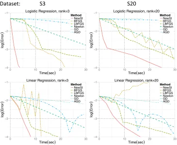
In this section, we validate the performance of Newton-Stein method through extensive numerical studies. We experimented on two commonly used GLM optimization problems, namely,Logistic Regression (LR) and Linear Regression (OLS). LR minimizes Equation 4 for the logistic function φ(z) = log(1 +ez), whereas OLS minimizes the same equation for φ(z) = z2/2. In the following, we briefly describe the algorithms that are used in the experiments:
• Newton’s Method (NM) uses the inverse Hessian evaluated at the current iterate, and may achieve local quadratic convergence. NM steps requireO(np2+p3) computation which makes it impractical for large-scale data sets.
• Broyden-Fletcher-Goldfarb-Shanno (BFGS) forms a curvature matrix by cultivating the information from the iterates and the gradients at each iteration. Under certain assumptions, the convergence rate is locally super-linear and the per-iteration cost is comparable to that of first order methods.
S3
Dataset:
S20
−4 −3 −2 −1
0 10 20 30
Time(sec)
log
(
E
rr
o
r
)
Method NewSt BFGS LBFGS Newton GD AGD
Logistic Regression, rank=3
−4
−3
−2
−1
0 10 20 30
Time(sec)
log
(
E
rr
o
r
)
Method
NewSt BFGS LBFGS Newton GD AGD Logistic Regression, rank=20
−4 −3 −2 −1
0 10 20 30
Time(sec)
log
(
E
rr
o
r
)
Method NewSt BFGS LBFGS Newton GD AGD
Linear Regression, rank=3
−4 −3 −2 −1
0 10 20 30
Time(sec)
log
(
E
rr
o
r
)
Method NewSt BFGS LBFGS Newton GD AGD Linear Regression, rank=20
Figure 2: Performance of various optimization methods on two different simulated data sets. Red straight line represents the Newton-Stein method (NewSt ). y and x
axes denote log10(kβˆt−β∗k2) and time elapsed in seconds, respectively.
• Gradient Descent (GD) update is proportional to the negative of the full gradient evaluated at the current iterate. Under smoothness assumptions, GD achieves a locally linear convergence rate, withO(np) per-iteration cost.
• Accelerated Gradient Descent (AGD) is proposed by Nesterov (Nesterov, 1983), which improves over the gradient descent by using a momentum term. Performance of AGD strongly depends of the smoothness of the function.
For all the algorithms, we use a constant step size that provides the fastest convergence. We use the Newton-Stein method with eigenvalue thresholding as described in Section 4.4. The parameters such as sub-sample size |S|, and rank r are selected by following the guidelines described in Section 4.4. The rank threshold r (which is an input to the eigenvalue thresholding) is specified at the title of each plot.
5.1 Simulations With Synthetic Data Sets
CT Slices
Dataset:
Covertype
−4
−3
−2
−1
0
0.0 2.5 5.0 7.5 10.0
Time(sec)
log
(
E
rr
o
r
)
Method NewSt BFGS LBFGS Newton GD AGD Logistic Regression, rank=40
−4
−3
−2
−1
0
0 10 20 30
Time(sec)
log
(
E
rr
o
r
)
Method NewSt BFGS LBFGS Newton GD AGD Logistic Regression, rank=2
−4 −3 −2 −1 0 1 2
0 1 2 3 4 5
Time(sec)
log
(
E
rr
o
r
)
Method
NewSt BFGS LBFGS Newton GD AGD Linear Regression, rank=40
−4 −3 −2 −1
0 1 2 3 4 5
Time(sec)
log
(
E
rr
o
r
)
Method NewSt BFGS LBFGS Newton GD AGD Linear Regression, rank=2
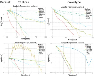
Figure 3: Performance of various optimization methods on two different real data sets ob-tained from Lichman, 2013. Red straight line represents the Newton-Stein method (NewSt ). y and x axes denote log10(kβˆt−β∗k2) and time elapsed in seconds, respectively.
for S20. To generate the covariance matrix, we first generate a random orthogonal matrix, sayM. Next, we generate a diagonal matrix Λthat contains the eigenvalues, i.e., the first
r diagonal entries are chosen to be large, and rest of them are equal to 1. Then, we let Σ =MΛMT. For dimensions of the data sets, see Table 2. We also emphasize that the data dimensions are chosen so that Newton’s method still does well.
The simulation results are summarized in Figure 2. Further details regarding the exper-iments can be found in Table 1. We observe that Newton-Stein method (NewSt) provides a significant improvement over the classical techniques.
5.2 Experiments With Real Data Sets
We experimented on two real data sets where the data sets are downloaded from UCI repository (Lichman, 2013). Both data sets satisfy n p, but we highlight the difference between the proportions of dimensions n/p. See Table 2 for details.
We observe that Newton-Stein method performs better than classical methods on real data sets as well. More specifically, the methods that come closer to NewSt is Newton’s method for moderate nand p and BFGS whenn is large.
The optimal step-size for Newton-Stein method will typically be larger than 1 which is mainly due to eigenvalue thresholding operation. This feature is desirable if one is able to obtain a large step-size that provides convergence. In such cases, the convergence is likely to be faster, yet more unstable compared to the smaller step size choices. We observed that similar to other second order algorithms, Newton-Stein method is also susceptible to the step size selection. If the data is not well-conditioned, and the sub-sample size is not sufficiently large, algorithm might have poor performance. This is mainly because the sub-sampling operation is performed only once at the beginning. Therefore, it might be good in practice to sub-sample once in every few iterations.
Data set S3 S20
Type LR LS LR LS
Method Time(sec) Iter Time(sec) Iter Time(sec) Iter Time(sec) Iter NewSt 10.637 2 8.763 4 23.158 4 16.475 10 BFGS 22.885 8 13.149 6 40.258 17 54.294 37 LBFGS 46.763 19 19.952 11 51.888 26 33.107 20 Newton 55.328 2 38.150 1 47.955 2 39.328 1 GD 865.119 493 155.155 100 1204.01 245 145.987 100 AGD 169.473 82 65.396 42 182.031 83 56.257 38
Data set CT Slices Covertype
Type LR LS LR LS
Method Time(sec) Iter Time(sec) Iter Time(sec) Iter Time(sec) Iter NewSt 4.191 32 1.799 11 16.113 31 2.080 5 BFGS 4.638 35 4.525 37 21.916 48 2.238 3 LBFGS 26.838 217 22.679 180 30.765 69 2.321 3 Newton 5.730 3 1.937 1 122.158 40 2.164 1 GD 96.142 1156 61.526 721 194.473 446 22.738 60 AGD 96.142 880 45.864 518 80.874 186 32.563 77
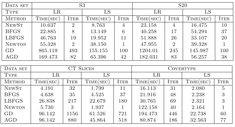
Table 1: Details of the experiments presented in Figures 2 and 3.
Data set n p Reference, UCI repo (Lichman, 2013) CT slices 53500 386 Graf et al., 2011
Covertype 581012 54 Blackard and Dean, 1999
S3 500000 300 3-spiked model, (Donoho et al., 2013) S10 500000 300 10-spiked model, (Donoho et al., 2013) S20 500000 300 20-spiked model, (Donoho et al., 2013)
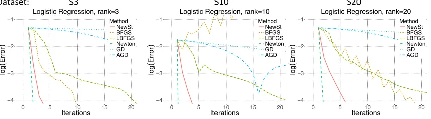
5.3 Analysis of Number of Iterations
We provide additional plots to better understand the convergence behavior of the algo-rithms. Plots in Figure 4 show the decrease in log10(kβˆt −β0k2) error over iterations (instead of time elapsed).
S3
Dataset: S10 S20
−4 −3 −2 −1
0 5 10 15 20
Iterations
log
(
E
rr
o
r
)
Method NewSt BFGS LBFGS Newton GD AGD Logistic Regression, rank=3
−4 −3 −2 −1
0 5 10 15 20
Iterations
log
(
E
rr
o
r
)
Method NewSt BFGS LBFGS Newton GD AGD Logistic Regression, rank=10
−4
−3
−2
−1
0 5 10 15 20
Iterations
log
(
E
rr
o
r
)
Method NewSt BFGS LBFGS Newton GD AGD Logistic Regression, rank=20
Figure 4: Figure shows the convergence behavior over the number of iterations. y and x
axes denote log10(kβˆt−β∗k2) and the number iterations, respectively.
We observe from the plots that Newton’s method enjoys the fastest convergence rate as expected. The one that is closest to Newton’s method is the Newton-Stein method. This is because the Hessian estimator used by Newton-Stein method better approximates the true Hessian as opposed to Quasi-Newton methods. We emphasize thatx axes in Figure 4 denote the number of iterations whereas in figures shown previously in this sectionx axes were the time elapsed.
6. Discussion
In this paper, we proposed an efficient algorithm for training GLMs. We call our algorithm Newton-Stein method (NewSt ) as it takes a Newton-type step at each iteration relying on a Stein-type lemma. The algorithm requires a one time O(|S|p2) cost to estimate the co-variance structure andO(np) per-iteration cost to form the update equations. We observe that the convergence of Newton-Stein method has a phase transition from quadratic rate to linear rate. This observation is justified theoretically along with several other guaran-tees for the bounded as well as the sub-Gaussian covariates such as per-step convergence bounds, conditions for local rates and global convergence with line search, etc. Parame-ter selection guidelines of Newton-Stein method are based on our theoretical results. Our experiments show that Newton-Stein method provides significant improvement over the classical optimization methods.
Acknowledgments
The author is grateful to Mohsen Bayati and Andrea Montanari for stimulating conversa-tions on the topic of this work. The author would like to thank Bhaswar B. Bhattacharya and Qingyuan Zhao for carefully reading this article and providing valuable feedback.
Appendix A. Preliminary Concentration Inequalities
In this section, we provide several concentration bounds that will be useful throughout the proofs. We start by defining a special class of random variables.
Definition 10 (Sub-Gaussian) A random variable x ∈ R is called sub-Gaussian if it satisfies
E[|x|m]1/m≤K √
m, m≥1,
for some finite constant K. The smallest such K is the sub-Gaussian norm of x and it is denoted by kxkψ2. Similarly, a random vector y∈R
p is called sub-Gaussian if there exists
a constantK0>0 such that
sup
v∈Sp−1
khy, vikψ2 ≤K 0
.
Definition 11 (Sub-exponential) A random variable x ∈R is called sub-exponential if
it satisfies
E[|x|m]1/m≤Km, m≥1,
for some finite constant K. The smallest such K is the sub-exponential norm of x and it is denoted by kxkψ1. Similarly, a random vector y ∈ Rp is called sub-exponential if there
exists a constant K0 >0 such that
sup
v∈Sp−1
khy, vikψ1 ≤K 0
.
We state the following Lemmas from Vershynin, 2010 for the convenience of the reader (i.e., See Theorem 5.39 and the following remark for sub-Gaussian distributions, and The-orem 5.44 for distributions with arbitrary support):
Lemma 12 (Vershynin, 2010) Let S be an index set and xi ∈ Rp for i ∈ S be i.i.d.
sub-Gaussian random vectors with
E[xi] = 0, E[xixTi] =Σ, kxikψ2 ≤K.
There exists constants c, C depending only on the sub-Gaussian norm K such that with probability 1−2e−ct2,
ΣbS−Σ
2 ≤max δ, δ 2
where δ=C
r
p
|S|+
t
p
|S|.
Remark 13 We are interested in the case whereδ <1, hence the right hand side becomes
max δ, δ2
= δ. In most cases, we will simply let t = √p and obtain a bound of order
p
The following lemma is an analogue of Lemma 12 for covariates sampled from arbitrary distributions with bounded support.
Lemma 14 (Vershynin, 2010) Let S be an index set and xi ∈ Rp for i ∈ S be i.i.d.
random vectors with
E[xi] = 0, ExixTi
=Σ, kxik2≤ √
K a.s.
Then, for some absolute constant c, with probability 1−pe−ct2, we have
bΣS−Σ
2≤max
kΣk12/2δ, δ2 where δ=t
s
K
|S|.
Remark 15 We will choose t = p3 log(p)/c which will provide us with a probability of
1−1/p2. Therefore, if the sample size is sufficiently large, i.e., |S| ≥ 3Klog(p)
ckΣk2 =O(Klog(p)/kΣk2),
we can estimate the true covariance matrix quite well for arbitrary distributions with bounded support. In particular, with probability 1−1/p2, we obtain
bΣS−Σ
2 ≤c 0
s
log(p) |S| ,
where c0 =p3KkΣk2/c.
In the following, we will focus on empirical processes and obtain uniform bounds for proposed Hessian approximation. To that extent, we provide a few basic definitions which will be useful later in the proofs. For a more detailed discussion on the machinery used throughout the next section, we refer reader to Van der Vaart, 2000.
Definition 16 On a metric space (X, d), for > 0, T ⊂ X is called an -net over X if
∀x∈X, ∃t∈T such that d(x, t)≤.
In the following, we will useL1distance between two functionsf andg, namelyd(f, g) =
R
|f−g|. Note that the same distance definition can be carried to random variables as they are simply real measurable functions. The integral takes the form of expectation.
Definition 17 Given a function class F, and any two functions l and u (not necessarily in F), the bracket [l, u] is the set of all f ∈ F such that l ≤ f ≤u. A bracket satisfying l≤u and R|u−l| ≤is called an -bracket in L1. The bracketing number N[](,F, L1) is
the minimum number of different -brackets needed to cover F.
Appendix B. Main Lemmas
B.1 Concentration of Covariates With Bounded Support
Lemma 18 Let xi ∈ Rp, for i = 1,2, ..., n, be i.i.d. random vectors supported on a ball
of radius √K, with mean 0, and covariance matrix Σ. Further, let f : R → R be a
uniformly bounded function such that for someB >0, we havekfk∞< Bandf is Lipschitz
continuous with constant L. Then, for sufficiently large n, there exist constants c1, c2, c3
such that
P sup
β∈Bp(R)
1 n n X i=1
f(hxi, βi)−E[f(hx, βi)]
> c1
r
plog(n)
n
!
≤c2e−c3p,
where the constants depend only on the bound B.
Proof We start by using the Lipschitz property of the function f, i.e., ∀β, β0∈Bp(R),
f(hx, βi)−f(hx, β0i)
≤Lkxk2kβ−β0k2,
≤L√Kkβ−β0k2,
where the first inequality follows from Cauchy-Schwartz. Now letT∆be a ∆-net overBp(R).
Then∀β ∈Bp(R),∃β0 ∈T∆such that the right hand side of the above inequality is smaller than ∆L√K. Then, we can write
1 n n X i=1
f(hxi, βi)−E[f(hx, βi)]
≤ 1 n n X i=1
f(hxi, β0i)−E[f(hx, β0i)]
+ 2∆L
√
K. (14)
By choosing
∆ = 4L√K,
and taking supremum over the corresponding β sets on both sides, we obtain the following inequality
sup
β∈Bn(R)
1 n n X i=1
f(hxi, βi)−E[f(hx, βi)]
≤ max
β∈T∆
1 n n X i=1
f(hxi, βi)−E[f(hx, βi)]
+ 2.
Now, since we havekfk∞≤B and for a fixedβ andi= 1,2, ..., n, the random variables f(hxi, βi) are i.i.d., by the Hoeffding’s concentration inequality, we have
P 1 n n X i=1
f(hxi, βi)−E[f(hx, βi)]
> /2
!
≤2 exp
−n 2 8B2
.
Combining Equation 14 with the above result and a union bound, we easily obtain
P sup
β∈Bn(R)
1 n n X i=1
f(hxi, βi)−E[f(hx, βi)]
> !
≤P max
β∈T∆
1 n n X i=1
f(hxi, βi)−E[f(hx, βi)]
> /2
!
≤2|T∆|exp
−n 2 8B2
where ∆ =/4L√K.
Next, we apply Lemma 33 and obtain that
|T∆| ≤
R√p
∆
p
=
R√p /4L√K
p
.
We require that the probability of the desired event is bounded by a quantity that attains an exponential decay with rate O(p). This can be attained if
2≥ 8B 2p
n log
4eLR√K√p/.
Assuming that n is sufficiently large, and using Lemma 34 with a = 8B2p/n and b = 4eLR√Kp, we obtain that should be
=
s
4B2p
n log
30L2R2Kn
B2
=O
r
plog(n)
n
!
.
When n >30L2R2K/B2, we obtain
P sup
β∈Bn(R)
1
n
n X
i=1
f(hxi, βi)−E[f(hx, βi)]
>3B
r
plog(n)
n
!
≤2e−p.
In the following, we state similar bounds on functions of the following form
x→f(hx, βi)hx, vi2,
which appear in the summation that form the Hessian matrix.
Lemma 19 Let xi ∈ Rp, for i = 1, ..., n, be i.i.d. random vectors supported on a ball of
radius √K, with mean 0, and covariance matrix Σ. Also let f : R → R be a uniformly
bounded function such that for some B > 0, we have kfk∞ < B and f is Lipschitz
con-tinuous with constant L. Then, for v∈Sp−1 and sufficiently large n, there exist constants
c1, c2, c3 such that
P sup
β∈Bp(R)
1
n
n X
i=1
f(hxi, βi)hxi, vi2−E[f(hx, βi)hx, vi2]
> c1
r
plog (n)
n
!
≤c2e−c3p,
where the constants depend only on the bound B and the radius √K.
Proof As in the proof of Lemma 18, we start by using the Lipschitz property of the functionf, i.e., ∀β, β0 ∈Bp(R),
kf(hx, βi)hx, vi2−f(hx, β0i)hx, vi2k
For a net T∆,∀β ∈Bp(R), ∃β0 ∈T∆ such that right hand side of the above inequality is smaller than ∆LK1.5. Then, we can write
1 n n X i=1
f(hxi, βi)hxi, vi2−E[f(hx, βi)hx, vi2]
≤ 1 n n X i=1
f(hxi, β0i)hxi, vi2−E[f(hx, β0i)hx, vi2]
+ 2∆LK1.5. (15) This time, we choose
∆ = 4LK1.5,
and take the supremum over the corresponding feasibleβ-sets on both sides,
sup
β∈Bp(R)
1 n n X i=1
f(hxi, βi)hxi, vi2−E[f(hx, βi)hx, vi2]
≤max
β∈T∆
1 n n X i=1
f(hxi, βi)hxi, vi2−E[f(hx, βi)hx, vi2] + 2.
Now, since we havekfk∞≤B and for fixedβ andv,i= 1,2, ..., n,f(hxi, βi)hxi, vi2 are
i.i.d. random variables. By the Hoeffding’s concentration inequality, we write
P 1 n n X i=1
f(hxi, βi)hxi, vi2−E[f(hx, βi)hx, vi2]
> /2
!
≤2 exp
− n 2 8B2K2
.
Using Equation 15 and the above result combined with the union bound, we easily obtain
P sup
β∈Bp(R)
1 n n X i=1
f(hxi, βi)hxi, vi2−E[f(hx, βi)hx, vi2] > !
≤P max
β∈T∆
1 n n X i=1
f(hxi, βi)hxi, vi2−E[f(hx, βi)hx, vi2]
> /2
!
≤2|T∆|exp
− n 2 8B2K2
,
where ∆ =/4LK1.5. Using Lemma 33, we have |T∆| ≤
R√p
∆
p
=
R√p
/4LK1.5
p
.
As before, we require that the right hand side of above inequality gets a decay with rate O(p). Using Lemma 34 witha= 8B2K2p/nand b= 100LRK1.5√p, we obtain that
should be
=
s
4B2K2p
n log
502L2R2Kn
B2
=O
r
plog(n)
n
!
When n >50LRK1/2/B, we obtain
P sup
β∈Bp(R)
1
n
n X
i=1
f(hxi, βi)hxi, vi2−E[f(hx, βi)hx, vi2]
>4BK
r
plog(n)
n
!
≤2e−3.2p.
The rate−3.2p will be important later.
B.2 Concentration of Sub-Gaussian Covariates
In this section, we derive the analogues of the Lemmas 18 and 19 for sub-Gaussian covariates. Note that the Lemmas in this section are more general in the sense that they also cover the case where the covariates have bounded support. As a result, the resulting convergence coefficients are worse compared to the previous section.
Lemma 20 Let xi ∈Rp, for i= 1, ..., n, be i.i.d. sub-Gaussian random vectors with mean 0, covariance matrix Σ and sub-Gaussian norm K. Also let f : R → R be a uniformly
bounded function such that for some B >0, we have kfk∞< B and f is Lipschitz
contin-uous with constant L. Then, there exists absolute constants c1, c2, c3 such that
P sup
β∈Bn(R)
1
n
n X
i=1
f(hxi, βi)−E[f(hx, βi)]
> c1
r
plog(n)
n
!
≤c2e−c3p,
where the constants depend only on the eigenvalues of Σ, bound B and radius R and sub-Gaussian norm K.
Proof We start by defining the brackets of the form
lβ(x) =f(hx, βi)−
kxk2 4E[kxk2]
,
uβ(x) =f(hx, βi) +
kxk2 4E[kxk2].
Observe that the size of bracket [`β, uβ] is /2, i.e., E[uβ −`β] = /2. Now let T∆ be a ∆-net over Bp(R) where we use ∆ = /(4LE[kxk2]). Then ∀β ∈ Bp(R), ∃β0 ∈ T∆ such that f(h·, βi) falls into the bracket [`β0, uβ0]. This can be seen by writing out the Lipschitz
property of the function f. That is,
|f(hx, βi)−f(hx, β0i)| ≤Lkxk2kβ−β0k2, ≤∆Lkxk2,
where the first inequality follows from Cauchy-Schwartz. Therefore, we conclude that
for the function classF ={f(h·, βi) :β ∈Bp(R)}. We further have ∀β ∈Bp(R),∃β0 ∈T∆ such that 1 n n X i=1
f(hxi, βi)−E[f(hx, βi)]≤ 1
n
n X
i=1
uβ0(xi)−E[uβ0(x)] +
2, 1 n n X i=1
f(hxi, βi)−E[f(hx, βi)]≥
1
n
n X
i=1
lβ0(xi)−E[lβ0(x)]−
2.
Using the above inequalities, we have,∀β∈Bp(R),∃β0∈T∆
(" 1 n n X i=1
uβ0(xi)−E[uβ0(x)]
#
> /2
) ∪ (" −1 n n X i=1
lβ0(xi) +E[lβ0(x)]
#
> /2
) ⊃ ( 1 n n X i=1
f(hxi, βi)−E[f(hx, βi)]
> ) .
By the union bound, we obtain
P max
β∈T∆
" 1 n n X i=1
uβ(xi)−E[uβ(x)] #
> /2
!
+P max
β∈T∆
" −1 n n X i=1
lβ(xi) +E[lβ(x)] #
> /2
!
≥P sup
β∈Bp(R)
1 n n X i=1
f(hxi, βi)−E[f(hx, βi)] > ! . (16)
In order to complete the proof, we need concentration inequalities foruβ and lβ. We state
the following lemma.
Lemma 21 There exists a constantC depending on the eigenvalues ofΣandB such that, for each β ∈Bp(R) and for some0< <1, we have
P 1 n n X i=1
uβ(xi)−E[uβ(x)]
> /2
!
≤2e−Cn2,
P 1 n n X i=1
lβ(xi)−E[lβ(x)]
> /2
!
≤2e−Cn2,
where
C = c
B+ √
2K
4µ/√p 2
for an absolute constant c.
Proof By the relation between sub-Gaussian and sub-exponential norms, we have
kkxk2k2ψ2 ≤ kkxk 2 2kψ1 ≤
p X
i=1
kx2ikψ1, (17)
≤2
p X
i=1
kxik2ψ2, ≤2K2p.
Therefore kxk2 −E[kxk2] is a centered sub-Gaussian random variable with sub-Gaussian norm bounded above by 2K√2p. We have,
E[kxk2] =µ.
Note thatµis actually of order√p. Assuming that the left hand side of the above equality is equal to √pK0 for some constant K0 > 0, we can conclude that the random variable
uβ(x) =f(hx, βi) +
kxk2
4E[kxk2] is also sub-Gaussian with
kuβ(x)kψ2 ≤B+
4E[kxk2]
kkxk2kψ2 ≤B+
4√pK0K
p
2p
≤B+C0
whereC0 =√2K/4K0 is a constant and we also assumed <1. Now, define the function
gβ(x) =uβ(x)−E[uβ(x)].
Note thatgβ(x) is a centered sub-Gaussian random variable with sub-Gaussian norm
kgβ(x)kψ2 ≤2B+ 2C 0.
Then, by the Hoeffding-type inequality for the sub-Gaussian random variables, we obtain
P
1
n
n X
i=1
gβ(xi)
> /2
!
≤2e−cn2/(B+C0)2
wherec is an absolute constant. The same argument also holds for lβ(x).
Using the above lemma with the union bound over the set T∆, we can write
P sup
β∈Bp(R)
1
n
n X
i=1
f(hxi, βi)−E[f(hx, βi)]
>
!
≤4|T∆|e−Cn 2
Since we can also write, by Lemma 33
|T∆| ≤
R√p
∆
p
≤
4RL
E[kxk2] √
p
p
,
≤ 4 √
2RLKp
!p
,
and we observe that, for the constantc0= 4√2RLK,
P sup
β∈Bn(R)
1
n
n X
i=1
f(hxi, βi)−E[f(hx, βi)]
>
!
≤4 4 √
2RLKp
!p
e−Cn2,
= 4 expplog(c0p/)−Cn2 .
We will obtain an exponential decay of order p on the right hand side. For some constant
h depending onn andp, if we choose=hp, we need
h2 ≥ 1
Cnplog(c 0
/h).
By the Lemma 34, choosing h2 = log(2c02Cnp)/(2Cnp), we satisfy the above requirement. Note that fornlarge enough, the condition of the lemma is easily satisfied. Hence, for
2 = plog(2c 02Cnp) 2Cn =O
plog(n)
n
,
we obtain that there exists constants c1, c2, c3 such that
P sup
β∈Bn(R)
1
n
n X
i=1
f(hxi, βi)−E[f(hx, βi)]
> c1
r
plog(n)
n
!
≤c2e−c3p,
where
c1= 3
B+
√ 2K
4√Tr(Σ)/p−16K2
2
2c , c2=4,
c3= 1
2log(7)≤ 1
2log(log(64R
2L2K2C) + 6 log(p)). when p > eand 64R2L2K2C > e.
In the following, we state the concentration results on the unbounded functions of the form
x→f(hx, βi)hx, vi2.
Lemma 23 Let xi, for i = 1, ..., n, be i.i.d sub-Gaussian random variables with mean 0,
covariance matrixΣand sub-Gaussian normK. Also letf :R→Rbe a uniformly bounded
function such that for some B >0, we have kfk∞ < B and f is Lipschitz continuous with
constant L. Further, let v ∈ Rp such that kvk
2 = 1. Then, for n, p sufficiently large
satisfying
n0.2/log(n)&p,
there exist constants c1, c2 depending on L, B, R and the eigenvalues of Σ such that, we
have
P sup
β∈Bp(R)
1
n
n X
i=1
f(hxi, βi)hxi, vi2−E[f(hx, βi)hx, vi2]
> c1
r
p
n0.2log (n)
!
≤c2e−p.
Proof We define the brackets of the form
lβ(x) =f(hx, βi)hx, vi2−
kxk3 2 4Ekxk32
,
uβ(x) =f(hx, βi)hx, vi2+
kxk3 2 4Ekxk3
2
, (18)
and we observe that the bracket [`β, uβ] has size/2 inL1, that is, E[|uβ(x)−lβ(x)|] =/2.
Next, for the following constant
∆ = 4LEkxk32
,
we define a ∆-net over Bp(R) and call it T∆. Then, ∀β ∈ Bp(R), ∃β0 ∈ T∆ such that
f(h·, βi)h·, vi2 belongs to the bracket [`
β0, uβ0]. This can be seen by writing the Lipschitz
continuity of the functionf, i.e.,
f(hx, βi)hx, vi2−f(hx, β0i)hx, vi2
=hx, vi2
f(hx, βi)−f(hx, β0i) ,
≤Lkxk22 kvk22 hx, β−β0i ,
≤Lkxk32kβ−β0k2,
≤∆Lkxk32,
where we used Cauchy-Schwartz to obtain the above inequalities. Hence, we may conclude that for the bracketing functions given in Equation 18, the corresponding bracketing number of the function class
F ={f(h·, βi)h·, vi2 :β∈Bp(R)}
is bounded above by the covering number of the ball of radius R for the given scale ∆ =
/(4LEkxk32
), i.e.,
Next, we will upper bound the target probability using the bracketing functions uβ, lβ.
We have ∀β ∈Bp(R),∃β0 ∈ T∆ such that 1
n
n X
i=1
f(hxi, βi)hxi, vi2−E[f(hx, βi)hx, vi2]≤ 1
n
n X
i=1
uβ0(xi)−E[uβ0(x)] +
2, 1 n n X i=1
f(hxi, βi)hxi, vi2−E[f(hx, βi)hx, vi2]≥ 1
n
n X
i=1
lβ0(xi)−E[lβ0(x)]−
2.
Using the above inequalities,∀β ∈Bp(R),∃β0 ∈ T∆, we can write (" 1 n n X i=1
uβ0(xi)−E[uβ0(x)]
#
> /2
) ∪ (" −1 n n X i=1
lβ0(xi) +E[lβ0(x)]
#
> /2
) ⊃ ( 1 n n X i=1
f(hxi, βi)hxi, vi2−E[f(hx, βi)hx, vi2]
> ) .
Hence, by the union bound, we obtain
P max
β∈T∆
" 1 n n X i=1
uβ(xi)−E[uβ(x)] #
> /2
!
+P max
β∈T∆
" −1 n n X i=1
lβ(xi) +E[lβ(x)] #
> /2
!
≥P sup
β∈Bp(R)
1 n n X i=1
f(hxi, βi)hxi, vi2−E[f(hx, βi)hx, vi2]
> ! . (19)
In order to complete the proof, we need one-sided concentration inequalities foruβ and lβ.
Handling these functions is somewhat tedious since kxk3
2 terms do not concentrate nicely. We state the following lemma.
Lemma 24 For givenα, >0, andnsufficiently large such that,ν(nα, p, , B, K,Σ)< /4
where
ν(nα, p, , B, K,Σ) =:2
nα+6BK 2p
c
exp
−c n
α
6BK2p
+ 2
(
nα+ 3K 2p
cTr(Σ)n
α/32/3
+ 3K 4p2
c2Tr(Σ)2
4/3n−α/3
)
exp −cTr(Σ)(n
α/)2/3 2K2p
!
.
Then, there exists constants c0, c00, c000 depending on the eigenvalues of Σ, B and K such that∀β, we have,
P 1
n
n X
i=1
uβ(xi)−E[uβ(x)]> /2 !
≤2 exp −c0nα/p
+ 2 exp−c00n2α/3−2/3+ exp −c000n1−2α2
,
and
P −1
n
n X
i=1
lβ(xi) +E[lβ(x)]> /2 !
≤2 exp −c0nα/p
+
2 exp
−c00n2α/3−2/3
Proof For the sake of simplicity, we define the functions ˜
uβ(w) =uβ(w)−E[uβ(x)],
˜
lβ(w) =lβ(w)−E[lβ(x)].
We will derive the result for the upper bracket, ˜u, and skip the proof for the lower bracket ˜
l as it follows from the same steps. We write,
P 1
n
n X
i=1 ˜
uβ(xi)> /2 !
≤P 1
n
n X
i=1 ˜
uβ(xi)> /2, max
1≤i≤n|u˜β(xi)|< n α
!
+P
max
1≤i≤n|u˜β(xi)| ≥n α
. (20)
We need to bound the right hand side of the above equation. For the second term, since ˜
uβ(xi)’s are i.i.d. centered random variables, we have
P
max
1≤i≤n|u˜β(xi)| ≥n α
=1−P
max
1≤i≤n|u˜β(xi)|< n α
,
=1−P(|u˜β(x)|< nα)n,
=1−(1−P(|u˜β(x)| ≥nα))n,
≤nP(|u˜β(x)| ≥nα).
Also, note that
|u˜β(x)| ≤Bkxk22+
kxk3 2 4Ekxk32
+E[uβ(x)],
≤Bkxk22+ kxk
3 2 4Ekxk32
+Bλmax(Σ) +/4.
Therefore, if t >3Bλmax(Σ) and for small, we can write
{|u˜β(x)|> t} ⊂
Bkxk22 > t/3 ∪
(
kxk
3 2 4Ekxk3
2
> t/3 )
. (21)
Since x is a sub-Gaussian random variable withkxkψ2 =K, we have
K = sup
w∈Sp−1
khw, xikψ2 =kxkψ2.
Using this and the relation between sub-Gaussian and sub-exponential norms as in Equa-tion 17, we have kkxk2k2ψ2 ≤2K2p. This provides the following tail bound for kxk2,
P(kxk2> s)≤2 exp
− cs 2 2pK2
wherec is an absolute constant. Using the above tail bound, we can write,
P
kxk22> 1
3Bt
≤2 exp
−c t
6BK2p
.
For the next term in Equation 21, we need a lower bound forEkxk32
. We use a modified version of the H¨older’s inequality and obtain
Ekxk32
≥Ekxk22
3/2
= Tr(Σ)3/2.
Using the above inequality, we can write
P kxk 3 2 4Ekxk3
2
> t/3 !
≤P
kxk32 > 4
3Tr(Σ)
3/2t
,
=P kxk2 >
4t
3
1/3
Tr(Σ)1/2
!
,
≤2 exp −cTr(Σ)(t/)
2/3 2K2p
!
,
wherec is the same absolute constant as in Equation 22. Now for α > 0 such that t = nα > 3Bλ
max(Σ) (we will justify this assumption for a particular choice of α later), we combine the above results,
P(|u˜β(x)|> t)≤2 exp
−c t
6BK2p
+ 2 exp −cTr(Σ)(t/)
2/3 2K2p
!
. (23)
Next, we focus on the first term in Equation 20. Let µ = E[˜uβ(x)I{|u˜β(x)|<nα}], and
write
P 1
n
n X
i=1 ˜
uβ(xi)>
2; max1≤i≤n|u˜β(xi)|< n α
!
≤P 1
n
n X
i=1 ˜
uβ(xi)I{|u˜β(xi)|<nα} >
2
!
,
=P 1
n
n X
i=1 ˜
uβ(xi)I{|u˜β(xi)|<nα}−µ >
2−µ
!
≤exp
−n 1−2α
2
2−µ
2
,
where we used the Hoeffding’s concentration inequality for the bounded random variables. Further, note that
0 =E[˜uβ(x)] =µ+E
h
˜
uβ(x)I{|u˜β(x)|>nα}
i
.
By Lemma 30, we can write
|µ|=
E
h
˜
uβ(x)I{|u˜β(x)|>nα}
i ≤n
α
P(|u˜β(x)|> nα) + Z ∞
nα P