Ouémé River Catchment SWAT Model at Bonou Outlet: Model Performance, Predictive Uncertainty and Multi-Site Validation

2018; 6(2): 61-77

http://www.sciencepublishinggroup.com/j/hyd doi: 10.11648/j.hyd.20180602.13

ISSN: 2330-7609 (Print); ISSN: 2330-7617 (Online)

Ouémé River Catchment SWAT Model at Bonou Outlet:

Model Performance, Predictive Uncertainty and Multi-Site

Validation

Berenger Arcadius Sêgnonnan Dègan

1, 2, *

, Eric Adéchina Alamou

3

, Yèkambèssoun N’Tcha M’Po

1

,

Abel Afouda

4

1_{Department of Applied Hydrology, Water National Institute, University of Abomey-Calavi, Abomey-Calavi, Benin}

2_{Department of Civil Engineering, Polytechnic School of Abomey-Calavi, University of Abomey-Calavi, Abomey-Calavi, Benin}

3_{Department of Civil Engineering, School of Roads and Buildings, University of Science Technology Engineering and Mathematics, Abomey,}

Benin

4_{Department of Sciences and Technics, University of Abomey-Calavi, Abomey-Calavi, Benin}

Email address:

*

Corresponding author

To cite this article:

Berenger Arcadius Sêgnonnan Dègan, Eric Adéchina Alamou, Yèkambèssoun N’Tcha M’Po, Abel Afouda. Ouémé River Catchment SWAT Model at Bonou Outlet: Model Performance, Predictive Uncertainty and Multi-Site Validation. Hydrology. Vol. 6, No. 2, 2018, pp. 61-77. doi: 10.11648/j.hyd.20180602.13

Received: July 23, 2018; Accepted: August 10, 2018; Published: September 5, 2018

Abstract:

In a soudano-guinean climate context, the Ouémé River Basin is simulated using the semi-distributed hydrological model SWAT to understand the rainfall-runoff process on this basin and also to assess this model performance on West Africa large areas basins at daily and monthly time steps. The inputs data consist of climatic data and rain gauge discharge records. The inputs records are long-term times series for the period 1979-2010, while the considered land use is just for the year 2003. After calibration and validation of the model, spatial calibration is also performed to appreciate this other feature of the model. It gives such acceptable and disputable results. Six (06) hypotheses have been emitted to analyze this performance loss. It comes out that hypothesis H5 results perform better both in calibration and validation. This hypothesis used data for the period 1993-2010 with 1993-2004 for calibration and 2005-2010 for validation; and considered the missing data in discharge records without any completion. Considering the internal rain gauge outlet performance for this hypothesis, the best is retained and the corresponded project is realized for each individual subbasin to see how best the model could simulate discharge for the Bétérou, Kaboua and Atchérigbé individual subbasins. Hypothesis H1; an assumption which considers missing discharge with data time period of 1982-2010 with 1982-1996 for calibration and 1997-2010 for validation; is the best for Bétérou and Kaboua, whereas H5 is better for Atchérigbé subbasin. Uncertainty analysis and Global Sensitivity Analysis were performed to appreciate what are this process occurring in the basin and how these results could be validated. A last comparison effort is performed with 10km rainfall grid for climatic rainfall data at the global catchment outlet; this approach does not improve results, while at internal outlet some improvements are observed.

Keywords:

SWAT, Ouémé RIVER, Hypothesis, Uncertainty, Sensitivity, Analysis

1. Introduction

World is nowadays affected by climate unmastered laws. This situation leads to serious modification of human beings. According to climate drought of 70’s and the flood occurring in the second normalized regime, a lot of researchers have

started work on understanding the phenomen of rainfall runoff by setting up some distributed, global, conceptual or physic based models which describes and estimated the different water cycle on a basin.

past decade, several countries have been severely affected in Asia (China, Bangladesh and Vietnam in 2002 for example), Europe (France, Germany, Hungary and the Czech Republic in 2000) and elsewhere in the world (Venezuela in 1999, Canada, 1996, United States, 2005, etc.). It is the most frequent natural hazard arising from meteorological conditions and affecting the greatest number of people on the planet [2]. From this point of view, these authors estimated that floods account for more than a third of all cataclysms recorded at the end of the 20th century. Floods permit to account for the occurrence duration of exceptional climatic events [3]. They arise every year to complicate our urban populations’ existence than the rural one [4]. Their uncontrolled feature increases the populations’ vulnerability, especially the poorest ones. Indeed, these Floods sweep away agricultural crops, fields, houses, and socio-economic infrastructure, making thus many climate refugees.

In sub-Saharan Africa, it is checked and admitted that many more populated town (Lagos, Douala, Lome, Abidjan, Cotonou, Freetown, etc.) are often and increasingly suffer from floods. In 2010, several towns in Benin, including the city of Cotonou, were affected by floods that induced 680,000 disaster victims and caused 15,000 homeless. Forty-six (46) people were dead and the needs to face the damages were estimated at over US $ 46,847,399 [5].

For controlling the flood problem, the rainfall-runoff process needs to be more understood. Many researchers in the world have already thought about this situation by realizing models for control the water cycle components. This one leads to another important topic that many researchers focus nowadays. It is related to better understanding the water cycle for estimating the fresh water availability. Rapid, and often, unpredictable changes with regard to freshwater supplies create uncertainties for water managers. As meeting future water demands becomes more uncertain, and water scarcity is continuously increasing [6], societies become more vulnerable to a wide range of risks associated with inadequate water supply in quantity and/or quality [7]. Benin also, like all the other West African countries, have faced severe droughts period in the 70’s and its hydrologic cycle have changed. These changes have affected the water resources of West African watersheds [8-10]). Therefore, in the context of sustainable development, it is important to understand the dynamics of water exchanges within the whole biophysical and socio-economic systems. This reinforces the need for hydrological modeling of our basins. Hydrological models are important tools for planning sustainable use of water resources to meet various demands.

To account for all of these, hydrological models need data records in time and space for the investigated basin. Due to limited data availability, Water resources managers are facing challenges in many river basins across the world. This situation is more pronounced in developing countries, where in many river basins, any runoff data are available [11-15] and the existing ones are of questionable quality or, short time series or incomplete. This general situation is amplified by the non-maintenance of the existing network stations, the

deterioration of some and the theft of equipment. According to this issue of missing rainfall data and may be in addiction missing river discharge data, hydrological modelling of small scale basin become difficult. Nowadays, there is a new research thematic, which consist of modelling a large scale basin and others small scale in order to find the relationship between hydrological modelling of any small scale located in the large one based on the parameters set ranges of the model. In the fifth assessment report on regional aspects of climate change, the Inter-Governmental Panel on Climate Change [16] has shown that adaptation to climate change in Africa is confronted with a number of challenges among which there is a significant data gap. Too many basins lack reliable data necessary to assess, in details, impacts of climate change on different components of the hydrological cycle and to develop strategies of adaptation related to each specific impact. Thus, it is important to predict hydrological variables in ungauged basins for building high adaptive capacity by improving: (i) water resources knowledge, planning, and management; (ii) identification and implementation of strategies of adaptation to climate change in the sector of water, and (iii) ecological studies for a sustainable development.

For this study purpose, the distributed watershed model ‘‘Soil and Water Assessment Tool’’ (SWAT) [17] was selected. The SWAT (Soil and Water Assessment Tool) model is a continuous-time, semi-distributed, process-based river basin model. It was developed to evaluate the effects of alternative

management decisions on water resources and

others examples of SWAT model calibration on the Niger River basin [24, 27-30], the Volta basin [24, 27, 29-33] and the Oueme catchment in Benin [30, 34-36].

Many scientific worked in modelling the water balance cycle components in our basin to account for fresh water sustainability, showed SWAT performance for simulating discharge at Bonou Outlet subbasin (Atchérigbé, Savè, Kaboua, Beterou and Upper Oueme catchment) [34-45]. They worked on short data time period and sometimes non-continuous. Just one of them modeled the large area at Bonou outlet [45]. The works address the chemical dimension of soil degradation, notably the soil organic N and P loads and delivered together with sediment at catchment outlet. Organic N and P loads highly depend on landscape heterogeneity and spatial patterns of hydrological processes which are well known to smooth out with increasing catchment size resulting in more uncertain model parameters (without physical meaning) and more uncertain impact calculations at large scale, but almost none of the available impact studies have addressed this scaling problem, what is offered in its study. But the scale effect according to model performance for discharge using the same land use map was not considered. This scaling effect of modelling is important according to model a sub catchment without discharge data for predictions. Also the previous studies on the Ouémé River catchment used Impetus database for land use and most of them used gridded CRU data for rainfall. The rainfall gauged network is very rarely used due to missing values and the rain gauges spatial density. In this study, a network of 35 stations is considered, where 24 stations data have less than 15% missing values, the other ones data records were completed using the regional vector method. According to previous studies, where generally the uncertainties indicators values weren’t mentioned, they have been brought and the method for calibration have been revised to take into account all the large literature on the modeling with SWAT across the world.

This study is focused on SWAT performance for Ouémé basin at the outlet of Bonou, the spatial validation and the prediction and uncertainties. The time series considered were long terms time series according to the first SWAT applications in United States and in opposition to the recent daily realized on this basin. More precisely, the objective of this study was to assess the performance of the SWAT model and its predictive uncertainty on the Ouémé basin at catchment and sub catchment levels. It means specifically to: (i) set up a hydrological model for the entire Ouémé catchment using the SWAT program; (ii) calibrate the model at the catchment outlet at daily and monthly time steps and assess the predictive performance and uncertainty; (iii) evaluate the spatial performance of the watershed-wide model within the catchment by validating it at five internal stations; and (iv) calibrate the model at the sub-catchments separately and provide a comparative assessment of the model performance at different spatial scales; (v) make assumptions on the data records time series to get the best performance according to the available input data.

The choice of parameters, their ranges, and the inputs files

chosen for setting up the models, the spatial validation, which account for scale and the model prediction and uncertainties, were all discussed to provide a solid tool to help for using SWAT in the catchment for future works.

Bossa et al. [46] used scale dependent catchment properties to derive SWAT model parameters (for ungauged basins) using uncertainty thresholds and statistical approaches. They stated that for environmental modeling it is important to know (1) how knowledge of different small-scale processes may efficiently contribute to the simulation of large-scale behavior and (2) how and with which uncertainties model parameters are transferable to ungauged catchments. Therefore, the present study will assess the SWAT performance for the large basin by making some assumptions. It will also analyze how this large scale effect could influence the performance of small scale effect and vis-versa.

2. Materials and Methods

2.1. The Study Area

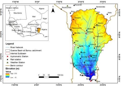
The Ouémé River basin at Bonou is located in the inter-tropical zone (between 07°58ʹN and 0°12ʹN), and has a wet and dry tropical climate. It covers an area of 46,920 km2 at the hydrometric station of Bonou. It stretches over 523 km [9, 47]. The aridity degree increases from south to north, and to a lesser extent, from west to east; according to the distance between the Atlantic Ocean and the latitude [48].

Mainly characterized by a Precambrian basement, consisting predominantly of complex migmatites granulites and gneisses, its soil is composed of fersialitic soils (ferruginous tropical soils) which are predominant, characterized by clay translocation and iron segregation (ferruginous tropical soils with iron segregation), which lead to a clear horizon differentiation [49]. A local scale description has shown a typical catena with lixisols/acrisols on the upper and middle slopes, following by plinthosols on the downslopes, gleysols in the inland valleys and fluvisols on the fluvial plain [50]. The landscape is characterized by forest islands, gallery forest, savannah, woodlands and agriculture, as well as pasture land.

1318.05 mm at Beterou station. Thus, the rainfall decreases middle ward and increases following an eastern south – western north gradient. The Ouémé River flows southward, and it is joined by two most important tributaries, Zou (150 Km) on the right bank and Okpara (200 km) on the left (Figure

1). Rainfall-runoff variability is high in this basin and leads to runoff coefficients that vary from 0.10 to 0.26 (of the total annual rainfall), with the lowest values in the savannahs and forest landscapes [44].

Figure 1. Location of the Ouémé River catchment at the Bonou outlet.

2.2. Input Data and Databases

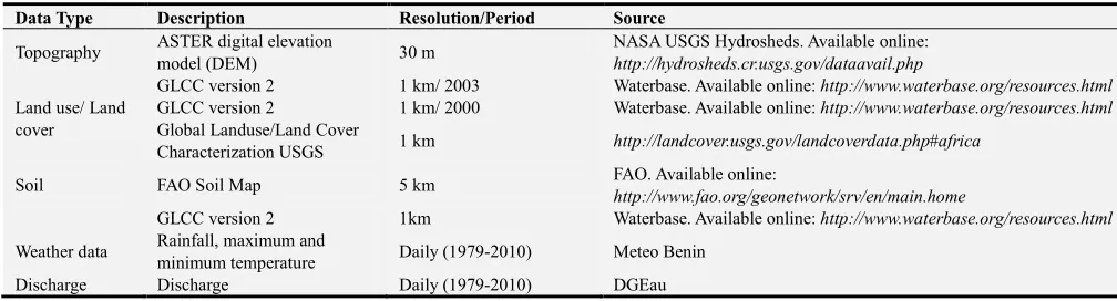
A combination of spatial and non-spatial input data from a variety of sources was used to set up the model. The spatial input data are described in Table 1. A 30 m DEM was obtained from the National Aeronautics and Space Administration (NASA) ASTER Global Digital Elevation Map to generate stream networks and watershed configurations, and to estimate topographic parameters. Three types of land use/Land cover were freely obtained on the waterbase mapwindow site and from usgs site. Two soil type maps were obtained; the first from the waterbase site and the second one from the Harmonized World Soil Database (HWSD) of FAO. Daily precipitation data from 25 rain gauges, as well as daily maximum and minimum temperature from four weather stations located mainly on the catchment were used as input. The location and spatial distribution of input precipitation and temperature stations are represented in Figure 1.

Rainfall and temperatures data were obtained from Benin National Meteorological Agency (Meteo Benin). Missing

rainfall data were completed using multi regression technic on the close stations data.

The daily discharge data were provided by the National Water Directorate (Direction Générale de l’Eau, DGEau). Twenty river gauges are available from the national observatory network in the Ouémé catchment (including the French Institute for Research and Development (IRD) river gauges). Discharge data for the period 1979–2010 are used for five stations (i.e. Atcherigbé, Bétérou, Bonou, Kaboua and Savè), whereas the time series for the period over 1986 – 2010 are used for Ahlan station.

purpose, the excel macro WGNmaker was used to calculate weather stations statistics needed to generate representative

daily climatic data.

Table 1. Input data of the SWAT model for the Oueme river catchment.

Data Type Description Resolution/Period Source

Topography ASTER digital elevation

model (DEM) 30 m

NASA USGS Hydrosheds. Available online:

http://hydrosheds.cr.usgs.gov/dataavail.php

Land use/ Land cover

GLCC version 2 1 km/ 2003 Waterbase. Available online: http://www.waterbase.org/resources.html

GLCC version 2 1 km/ 2000 Waterbase. Available online: http://www.waterbase.org/resources.html

Global Landuse/Land Cover

Characterization USGS 1 km http://landcover.usgs.gov/landcoverdata.php#africa

Soil FAO Soil Map 5 km FAO. Available online:

http://www.fao.org/geonetwork/srv/en/main.home

GLCC version 2 1km Waterbase. Available online: http://www.waterbase.org/resources.html

Weather data Rainfall, maximum and

minimum temperature Daily (1979-2010) Meteo Benin

Discharge Discharge Daily (1979-2010) DGEau

2.3. Model Description

The SWAT program is a comprehensive, semi-distributed, continuous-time, watershed processed-based model [18, 19, 51]. It is developed for assessing the impact of management and climate on water supplies, sediment, and agricultural chemical yields in watersheds and larger river basins. The hydrological component of SWAT allows explicit calculation of different water balance components, and subsequently water resources (e.g., blue and green waters) at a sub basin level. In SWAT, a watershed is divided into multiple sub basins, which are then further subdivided into hydrologic response units (HRUs) that consist of unique land use, management, topographical, and soil characteristics. Physical characteristics, such as slope, reach dimensions, and climatic data are considered for each sub basin. Simulation of watershed hydrology is done in the land phase, which controls the amount of water, sediment, nutrient, and pesticide loadings to the main channel in each sub basin, and in the routing phase, which is the movement of water, sediments, etc., through the streams of the sub basins to the outlets. Channel routing is simulated using the variable storage or Muskingum method.

The hydrological cycle is climate driven and provides moisture and energy inputs, such as daily precipitation, maximum/minimum air temperature, solar radiation, wind speed, and relative humidity that control the water balance. SWAT uses the data from the station nearest to the centroid of each sub basin. Hydrologic processes simulated by SWAT include canopy storage, surface runoff, infiltration and percolation. Optionally, pumping, pond storages, and reservoir operations could also be considered. The water balance for reservoirs includes inflow, outflow, rainfall on the surface, evaporation, seepage from the reservoir bottom, and diversions. The water in each HRU in SWAT is stored in four storage volumes: snow, soil profile (0 –2 m), shallow aquifer (typically 2–20 m), and deep aquifer.

Surface runoff from daily rainfall is estimated using a modified SCS curve number method, which estimates the amount of runoff based on local land use, soil type, and antecedent moisture condition. Peak runoff predictions are based on a modification of the Rational Formula [52]. The

watershed concentration time is estimated using Manning’s formula, considering both overland and channel flow. Snow is computed when temperatures are below freezing, and soil temperature is computed because it impacts water movement and the decay rate of residue in the soil.

Equation (MUSLE) [57] to predict sediment yield from the landscape. In addition, SWAT models the movement and transformation of several forms of nitrogen and phosphorus, pesticides, and sediment in the watershed. SWAT allows the user to define management practices taking place in every HRU. Once the loadings of water, sediment, nutrients, and pesticides from the land phase to the main channel have been determined, the loads are routed through the streams and reservoirs within the watershed. More details on the SWAT can be found in the theoretical documentation (http://swatmodel.tamu.edu) and in [17].

2.4. Model Setup

The catchment was delineated and divided into sub-catchments based on the DEM. A stream network was superimposed on the DEM in order to accurately delineate the location of the streams. The threshold drainage area was kept as default and additional outlets were considered at the location of stream gauging stations to enable comparison of measured discharge with SWAT results.

After combinations of the different land use/ land cover and soil type maps for the physical model setting and our SWAT2012.mdb database continuous modification to consider all classes of land use and soil, the retained final model is the one with the larger Nash Sutcliffe value at the first iteration. A Nash-Sutcliffe Efficiency (NSE) [58] was then calculated at Bonou catchment by comparing measured discharges against each default simulation and the one which will yield the highest NSE value will be kept for calibration and validation processes. This iteration was realized with no parameter value modification, just by considering the default value of the database. According to this methodology of processing, the combination of landuse map 2003 of waterbase.org and the FAO soil map got the larger NSE value: -2.32.

The whole catchment was discretized into 31 sub-catchments, which were further subdivided into 272 HRUs based on soil, land use, and slope combinations according to [59] and first iteration of 500 simulations results comparison using different land use soil type and slope thresholds. It is finally retained respectively the 5%, 5%, 2% thresholds for land use, soil type and slope respectively in the HRU creating step. Further parameters have been edited through the general watershed parameters and SWAT simulation menus.

The entire simulation period is from 1979 to 2010. As each station has data for different years, it is used about first half of the data for calibration and the second remaining for validation. The three first years are used for warm-up period to mitigate the initial conditions and were excluded from the analysis.

2.5. Calibration and Validation

2.5.1. Calibration Protocol for Large-Scale Distributed Models

To calibrate the model, we used the following general

approach:

1.Build the model with ArcSWAT using the best parameter estimates based on the available data, literature, and analyst’s expertise. There is always more than one data set (e.g., soil, land use, climate, etc.) available for a region. For Bonou, three different land use maps, two different soil maps were available (Table 1). Hence, initially several models were built and ran without any calibration (referred as the default model) with different databases. The model results were compared with observations (here discharge) and the best overall performing database was selected for further analysis. It should be noted that the performance of the default model should not be too drastically different from the measurement. If so, often calibration can be of little help. 2.Use the best default model to calibrate. Based on the performance of the default model at each outlet station, relevant parameters in the upstream sub basins are parameterized using the guidelines summarized in [60]. This procedure results in regionalization of the parameters.

3.Based on parameters identified in step 2 and one-at-a-time sensitivity analysis, initial ranges are assigned to parameters of significance. Experience and hydrological knowledge of the analyst is also of great asset in defining parameter ranges. In addition to the initial ranges, user-defined absolute parameter ranges are also defined for every SWAT parameter in SWAT-CUP [61], where parameters are not allowed to be outside of this range.

4.Once the model is parameterized and the ranges are assigned, the model is run 300–1000 times, depending on the number of parameters, the processing algorithm used, the speed of the model execution and the system capabilities.

5.After all simulations are completed; the post processing option in SWAT-CUP calculates the objective function and the 95PPU for all observed variables in the objective function. New parameter ranges are suggested by the program for a new iteration, which modifies the previous ranges focusing on the best parameter set of the current iteration [62, 63].

6.The suggested new parameter ranges could be modified by the user to stay in the Absolute parameters range and one-at-a-time sensitivity analysis again. A new iteration is then performed. The procedure continues until satisfactory results are reached (in terms of the P-factor and R-factor) or no further improvements are seen in the objective function. Normally, three to five iterations are sufficient for satisfactory results. More detailed information could be found in [62-64].

2.5.2. The SUFI2 Procedure

Multi-scale auto-calibration and uncertainty analysis were performed applying the SUFI-2 procedure (Sequential Uncertainty Fitting version 2, SWAT-CUP interface [65]).

and sensitivity analysis were performed within the SWAT Calibration and Uncertainty Programs SWAT-CUP version 2012 [65], using the Sequential Uncertainty Fitting version 2 (SUFI2) procedure [61]. In SUFI-2, uncertainty of input parameters are depicted as uniform distributions, while model output uncertainty is quantified by the 95% prediction uncertainty (95PPU) calculated at the 2.5% and 97.5% levels of the cumulative distribution of output variables obtained through Latin hypercube sampling. For the goodness of fit, as it compares two bands (the 95PPU for model simulation and the band representing measured data plus its error), Abbaspour coined two indices referred to as ‘‘P-factor’’ and ‘‘R-factor’’ [63]. The P-factor is the fraction of measured data (plus its error) bracketed by the 95PPU band and varies from 0 to 1, where 1 indicates 100% bracketing of the measured data within model prediction uncertainty (i.e., a perfect model simulation considering the uncertainty). For discharge, they recommend a value of >0.7 or 0.75 to be adequate. This of course, depends on the scale of the project and adequacy of the input and calibrating data. The R-factor on the other hand is the ratio of the average width of the 95PPU band and the standard deviation of the measured variable. A value of <1.5, again depending on the situation, would be desirable for this index [62, 63]. These two indices are used to judge the strength of the calibration and validation. A larger P-factor can be achieved at the expense of a larger R-factor. Hence, often a balance must be reached between the two. In the final iteration, where acceptable values of R-factor and P-factor are reached, the parameter ranges are taken as the calibrated parameters. SUFI-2 allows usage of ten different objective functions such as R2, Nash-Sutcliff (NSE), and mean square error (MSE). The likelihood functions selected here is principally the NSE as it is very commonly used and included in SWAT-CUP for SUFI2 performance assessment and is the best objective function for estimating the peaks. In this study, the number of model runs was set to 4 iterations of 500 simulations each one and the total sample of simulations were split into “behavioral” and “non-behavioral” based on a threshold value of 0.5, a minimum threshold for NSE recommended by Moriasi [66] for streamflow simulation to be judged as satisfactory on a monthly time step. In that case, only simulations which yielded a NSE > 0.5 are considered behavioral and kept for further analysis.

2.5.3. Calibration and Validation Steps

The first step in the calibration and validation process in SWAT is the determination of the most sensitive parameters for a given watershed or sub watershed. The sensitivity analysis is carried out by keeping all parameters constant to realistic values, while varying each parameter within the range assigned in step one. For each parameter about five simulations are performed by simply dividing the absolute ranges in equal intervals and allowing the midpoint of each interval to represent that interval. Plotting results of these simulations along with the observations on the same graph gives insight into the effects of the parameters on observed signals.

After retaining 17 parameters which could influence the discharge production according to all the found literature, one-at-time sensitivity analysis was performing to find the most sensitive range for each parameter. Then global calibration was performing using the 17 parameters. It has been called cal C.

According to former studies on the same area or on West Africa basins, 12 parameters were found to be used with certain range. Another calibration process was realized using them with their range. It has been called cal A. Still to be more focused on the SWAT project using data mentioned further, a new calibration process is set using the 12 parameters found but with one-at-time analysis results on their range. The new one is called cal B.

The 12 parameters used in previous studies were: SCS runoff curve number II (CN2), Manning’s “n” value for overland flow (OV_N), Average slope length (SLSUBBSN), Soil evaporation compensation factor (ESCO), Available water capacity of the soil layer (SOL_AWC), Groundwater delay (GW_DELAY), Threshold depth of water in the shallow aquifer required for return flow to occur (GWQMN), Threshold depth of water in the shallow aquifer for “revap” to occur (REVAPMN), Deep aquifer percolation fraction

(RCHRG_DP), Groundwater “revap” coefficient

(GW_REVAP), Surface runoff lag coefficient (SURLAG) and Baseflow alpha factor (ALPHA_BF). The five other added for cal C, are: Saturated hydraulic conductivity (SOL_K), Manning's "n" value for the main channel (CH_N2), Effective hydraulic conductivity in main channel alluvium (CH_K2), Maximum canopy storage (CANMX) and Average slope steepness (HRU_SLP).

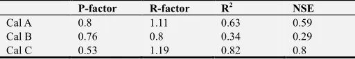
The various calibrations realized using 4 iterations results were shown on the Table 2. According to this table, Cal C gives the best performance by considering the Nash and R2 but the last one considering P-factor and R-factor. Cal C was then used for the validation processing.

The final step is validation for the component of interest (here discharge). Model validation is the process of demonstrating that a given site-specific model is capable of making sufficiently accurate simulations, although “sufficiently accurate” can vary based on project goals [67]. Validation involves running a model using parameters that were determined during the calibration process, and comparing the predictions to observed data not used in the calibration. In general, a good model calibration and validation should involve: (1) observed data that include wet, average, and dry years [68]; (2) multiple evaluation techniques [69-71]; (3) calibrating all constituents to be evaluated; and (4) verification that other important model outputs are reasonable.

Table 2. Preprocessing calibration to choose the parameters and range.

P-factor R-factor R2 NSE

Cal A 0.8 1.11 0.63 0.59

Cal B 0.76 0.8 0.34 0.29

2.6. Hypotheses for Results Improvement

Some hypotheses were made to justify the results case (i.e. the weak performance at daily time step). This unfitness of SWAT to perform well on this period is may be due to (1) rain and climatic stations network dispersion, should the rain data be spatialized using a grid?; (2) the land use map which is the same in all the simulation period; (3) missing data completion technic for rainfall and discharge records, shouldn’t the discharge missing data be completed? ; (4) semi-distributed feature of SWAT; (5) the long term time step in comparison with the former studies, the considered time period in validation, the non uniform regime of precipitations after the 2000, the presence of wet and dry years on this period. These last points highlight the data split procedure for calibration and validation. According to literatures, two thirds of flow series data is used for calibration and the last one for validation than half for each procedure. The entire period should be divided into calibration and validation periods while attempting to ensure that both periods have a similar number of wet and dry years and similar average water balances [18].

All these assumptions could not be verified; however some hypotheses have been done to achieve the study goals. According to the former studies on study areas with SWAT or on the West Africa, it is noticed different length (sometimes short) for data time period for simulation. Abbaspour [60] applied SWAT for water quality needs in Europe continent area. They used time period of 1970-2006 at monthly time step with first three years for warm-up period, two thirds for calibration and one third for validation. Gaborit [72] applied SWAT in model comparison approach to simulate the streamflow of the Saint-Charles River, located in Quebec, Canada. He used data for 1985-2005 time periods with first year for warm-up period, 1986-1995 for calibration and 1996-2005 for validation. He did not have good performance so he emitted the possibility to inverse the periods if the performance highly decreased on the validation period. Bossa [46] estimated scale effects for model soil and water degradation in Benin by using SWAT. These authors worked on 1998-2009 data periods with years 2007-2008 for calibration and 2001 to 2006 plus 2009 for validation. This approach does not follow any rule for choice. In an approach of modeling multiple hydrological ecosystem services, Duku [73] applied SWAT on the Bétérou basin in the time period of 1999-2011 with the two first years as warm-up period. Data period of 2001-2007 was considered for calibration, while the period 2008-2011 is used for validation. Hounkpè [74], applied SWAT on the Atchérigbé basin over the periods 1990 - 2010 ]. He used one year for warm-up period, 1999-2010 for calibration and 1991-1998 for validation. In order to contribute to the sustainable water resources management,

Sintondji [36] applied SWAT to the Ouémé basin at the outlet of Savè over the 1999-2006 time periods. They used the first two years for warm-up period, the period 2001-2004 for calibration and 2005-2006 for validation. Still to the contribution to the sustainable water resources management, Sintondji [75] applied SWAT to the Okpara basin at the outlet of Kaboua over the 1999-2007 time periods. Here, they just used the first year for warm-up period, the period 2000-2004 for calibration and 2005-2007 for validation. By evaluating SWAT model performance on multi-site validation of the Bani catchment, Begou [76] worked on 1983-1997 time periods for simulations with 1981-1982 for warm-up period, 1983-1992 for calibration and 1993-1997 for validation.

Stating on all the above, these hypotheses were made to try to find the best acceptable results at daily time step:

a)H1: streamflows data not completed, so with missing data on 1982-1996 for calibration and 1997-2010 for validation

b)H2: streamflows data not completed, so with missing data on 1997-2010 for calibration and 1982-1996 for validation

c)H3: streamflows data not completed, so with missing data on 1982-2001 for calibration and 2002-2010 for validation

d)H4: streamflows data not completed, so with missing data on 2002-2010 for calibration and 1982-2001 for validation

e)H5: streamflows data not completed, so with missing data on 1993-2004 for calibration and 2005-2010 for validation

f) H6: streamflows data not completed, so with missing data on 2005-2010 for calibration and 1993-2004 for validation.

3. Results

3.1. The Catchment Scale Model

3.1.1. Global Model Performance

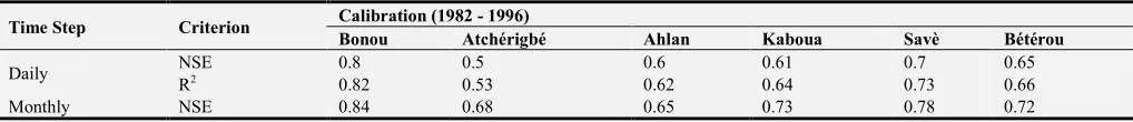
According to the results (Table 3), SWAT performs well to simulate discharge in calibration compared to the validation on this time period. However, the results for Bonou catchment was not good enough. At daily time step, in calibration all the results were satisfactory except for Atchérigbé sub catchment. At monthly time step, globally all the results were better in calibration than in validation; however the results at Atcherigbé were worst. An important notice is that the individual catchment which does not include another one, do not seem to be well simulated in comparison with Bonou, Ahlan and Savè.

Table 3. Model performance statistics for the Ouémé River catchment at Bonou, Ahlan, Atchérigbé, Savè, Kaboua and Bétérou discharge gauging stations.

Time Step Criterion Calibration (1982 - 1996)

Bonou Atchérigbé Ahlan Kaboua Savè Bétérou

Daily NSE 0.8 0.5 0.6 0.61 0.7 0.65

R2 _{0.82 0.53 0.62 0.64 0.73 0.66}

R2 _{0.86 0.69 0.67 0.74 0.83 0.73}

Time Step Criterion Validation (1997 - 2010)

Bonou Atchérigbé Ahlan Kaboua Savè Bétérou

Daily NSE 0.46 -0.25 0.48 0.22 0.42 0.41

R2 _{0.47 0.09 0.54 0.27 0.49 0.42}

Monthly NSE 0.52 -0.01 0.59 0.34 0.51 0.51

R2 _{0.54 0.2 0.6 0.36 0.55 0.51}

3.1.2. Spatial Validation

Some actions could be done to improve these results or better understand the reason behind these results. The first one is the motivation to compare the globally sub catchment SWAT performance with these individuals catchment SWAT model results. This operation is realized for Bétérou, Kaboua and Atchérigbé catchments.

The results were summarized in Table 4. Globally all the results obtained at the sub catchment applied models were better than those at internal sub basin considering the Bonou

applied Model except Bétérou at the daily time step. But in validation the results weren’t good yet.

According to this (SWAT performance on our large area basin), one could suppose that SWAT should not be concealed for hydrologic modelling on large area using so long term data at daily time step.

3.2. Bonou Outlet Comparative Hypotheses Results

After applying the different hypotheses, the results at the global model outlet of Bonou were shown in Table 5.

Table 4. Model performance statistics for the individual subbasins projects gauging stations.

Time Step Criterion Calibration (1982 - 1996) Validation (1997 - 2010)

Bétérou Kaboua Atchérigbé Bétérou Kaboua Atchérigbé

Daily NSE 0.7 0.74 0.67 0.41 0.32 0.09

R2 _{0.7 0.75 0.67 0.42 0.35 0.15}

Monthly NSE 0.84 0.83 0.88 0.63 0.37 0.22

R2 _{0.84 0.83 0.90 0.64 0.40 0.26}

Table 5. Hypotheses Model performance statistics for the Bonou catchment at daily time step.

Basin Model Bonou

Hypothesis H1 H2 H3 H4 H5 H6

Calibration

Data periods 1982-1996 1997-2010 1982-2001 2002-2010 1993-2004 2005-2010

Criterion NSE 0.82 0.43 0.82 0.47 0.86 0.65

R2 _{0.83 0.44 0.83 0.47 0.87 0.66}

Validation

Data periods 1997-2010 1982-1996 2002-2010 1982-2001 2005-2010 1993-2004

Criterion NSE 0.59 0.78 0.35 0.72 0.65 0.76

R2 _{0.60 0.8 0.38 0.77 0.66 0.79}

By analyzing this table, one could notice first by comparing H1 results with the previous SWAT applied model to the basin, that the completion technique was not such efficient mainly on the 1997-2010 periods’ data. Calibration on the recent part of the simulation period, do not give such good results. This case shows the unsteady character of this period mainly on the years 2000 to 2004 rainfall and discharge data. According to

all these hypotheses, H2 gives the best results in validation, while H5 gives the best results in calibration. Globally on the both periods SWAT performance H5 could be considered to be the most acceptable SWAT performance at the Bonou outlet. Visual graphical analyzes were also performed. At monthly time step, the results of Table 6, confirm these interesting results for hypothesis H5.

Table 6. Best Hypothesis Model performance statistics for the Bonou catchment at daily and monthly time steps.

Basin Model Bonou

Considered Outlet Bonou

Time Step Criterion Calibration H5 Validation H5

Daily NSE 0.86 0.65

R2 _{0.87 0.66}

Monthly NSE 0.90 0.67

R2 _{0.90 0.68}

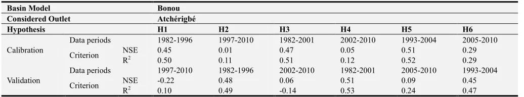
In the followings, the spatial validation is realized considering all these hypotheses results at the internal outlets in comparison with their subbasin applied SWAT model performance for the most acceptable results.

3.3. Spatial Validation

and the second step is to create the Sub basin SWAT model on this supposed “best hypothesis” for each subbasin to compare its performance to the internal sub basin performance of the Bonou SWAT model.

The results at the internal outlets of Bonou SWAT model on these hypotheses for the individual outlets of Bétérou, Kaboua and Atchérigbé are the following (Table 7, Table 8 and Table 9): According to these three tables, one starts by comparing H1 internal outlet results with the first Bonou internal outlets

results. For Bétérou subbasin, H1 calibration results are little bit better (NSE+0.01; R2+0.02), while H1 validation results are little bit worse (NSE-0.01; R2-0.02). But globally these two models for the sub basin are not so different. The completion was right done. For Kaboua sub basin, H1 calibration results are better (NSE+0.08; R2+0.06), while H1 validation results are little bit worse (NSE-0.02; R2-0.01). The completion was also almost right done.

Table 7. Hypotheses Model performance statistics for the Bonou catchment at the internal subbasin of Bétérou and daily time step.

Basin Model Bonou

Considered Outlet Bétérou

Hypothesis H1 H2 H3 H4 H5 H6

Calibration

Data periods 1982-1996 1997-2010 1982-2001 2002-2010 1993-2004 2005-2010

Criterion NSE 0.66 0.38 0.62 0.4 0.62 0.28

R2 _{0.68 0.38 0.63 0.41 0.69 0.29}

Validation

Data periods 1997-2010 1982-1996 2002-2010 1982-2001 2005-2010 1993-2004

Criterion NSE 0.40 0.64 0.38 0.63 0.23 0.67

R2 _{0.40 0.66 0.38 0.65 0.31 0.67}

Table 8. Hypotheses Model performance statistics for the Bonou catchment at the internal sub basin of Kaboua and daily time step.

Basin Model Bonou

Considered Outlet Kaboua

Hypothesis H1 H2 H3 H4 H5 H6

Calibration

Data periods 1982-1996 1997-2010 1982-2001 2002-2010 1993-2004 2005-2010

Criterion NSE 0.69 0.03 0.59 0.07 0.56 0.13

R2 _{0.70 0.11 0.6 0.13 0.57 0.14}

Validation

Data periods 1997-2010 1982-1996 2002-2010 1982-2001 2005-2010 1993-2004

Criterion NSE 0.20 0.66 -0.03 0.6 0.03 0.55

R2 _{0.26 0.67 0.07 0.61 0.09 0.57}

Table 9. Hypotheses Model performance statistics for the Bonou catchment at the internal sub basin of Atchérigbé and daily time step.

Basin Model Bonou

Considered Outlet Atchérigbé

Hypothesis H1 H2 H3 H4 H5 H6

Calibration

Data periods 1982-1996 1997-2010 1982-2001 2002-2010 1993-2004 2005-2010

Criterion NSE 0.45 0.01 0.47 0.05 0.51 0.29

R2 _{0.50 0.11 0.51 0.12 0.52 0.29}

Validation

Data periods 1997-2010 1982-1996 2002-2010 1982-2001 2005-2010 1993-2004

Criterion NSE -0.22 0.48 0.06 0.51 0.09 0.45

R2 _{0.10 0.49 -0.14 0.53 0.24 0.47}

For Atchérigbé subbasin, H1 calibration results are worse (NSE-0.05; R2-0.03), while H1 validation results are little bit better (NSE+0.03; R2+0.01). The completion was also right done. Globally H1 is not so different of the first Bonou SWAT model at the internal subbasin outlets. That means that it is just at Bonou outlet where there is an important difference mainly in validation (NSE+0.13; R2+0.13).

By comparing all the internal subbasins results for the different hypotheses, it is notified that H5 was not still the best option for future improvement. For Bétérou internal subbasin for example, H1 gives the best performance for calibration (NSE=0.66; R2=0.68), while H6 gives the best performance for validation (NSE=0.67; R2=0.67). But there is still a great problem about the recent period of the both in calibration or validation for all the hypotheses. For a best consensus, H1 is the best of the six hypotheses for Béterou subbasin outlet. For Kaboua internal subbasin, H1 gives the best performance for calibration (NSE=0.69; R2=0.70), while H2 gives the best performance for

objectives was to perform simulation of the last years’ peak flows, the options were between H1, H3 and H5. H5 is then chosen.

In summary, H1 gives the best performance for Bétérou and Atchérigbé internal sub basin, while H5 gives the best one for

Atchérigbé internal sub basin. The Béterou, Kaboua and Atchérigbé SWAT model performance using respectively hypothesis H1, H1 and H5 are summarized in Table 10:

Table 10. Best Hypothesis Model performance statistics for the Bonou, Atchérigbé and Kaboua.

Calibration Validation

Hypothesis H1 (1982 - 1996) H5 (1993 - 2004) H1 (1997 - 2010) H5 (2005 - 2010) Time Step Criterion Bétérou Kaboua Atchérigbé Bétérou Kaboua Atchérigbé

Daily NSE 0.69 0.83 0.58 0.40 0.33 0.39

R2 _{0.69 0.84 0.59 0.41 0.35 0.39}

Monthly NSE 0.79 0.91 0.82 0.57 0.38 0.60

R2 _{0.80 0.91 0.82 0.57 0.4 0.61}

This table clearly shows that lot of performance on each sub basin SWAT model positively change. For Bétérou SWAT model, one can see that its SWAT performance was not so different from the Bonou model internal Bétérou sub basin. It is almost the same (NSE+0.03; R2+0.01 for calibration and NSE+0.00; R2+0.01 for validation). But it could be noticed that important difference appears in Kaboua and Atchérigbé SWAT model performance. For Kaboua, at calibration a real increase is noticed (NSE+0.14; R2+0.14). It is most well simulated. For validation also, a real raise is realized (NSE+0.13; R2+0.09), but it is not enough to say this is well simulated. For Atchérigbé also something important could be seen as for calibration (NSE+0.07; R2+0.07) than for validation (NSE+0.3; R2+0.15). A great increase is obtained for simulation but it’s still not well simulated.

Generally all the applied models performed well at monthly

time step except at Kaboua where the decrease from calibration to validation is too huge. Something important such as important loss or important variation of land use or bad quality of the recorded data should be behind this inability to perform on last recent years setting on the historic data.

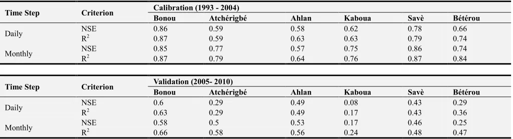
3.4. Using 10km Grid Network Rainfall

Here, one try to check the real influence of grid data in SWAT model using our rain gauges network for input. To this end, 10km grid data has been achieved base on the rain gauges network using IDW spatialization technique. Calibration and validation have been performed after setting up the ArcSwat physical model. The post processing results at the global outlet and sub basin ones have been highlighted in Table 11.

Table 11.H5 Hypothesis Model performance statistics for the Bonou catchment at daily and monthly time steps using spatialized rainfall input.

Time Step Criterion Calibration (1993 - 2004)

Bonou Atchérigbé Ahlan Kaboua Savè Bétérou

Daily NSE 0.86 0.59 0.58 0.62 0.78 0.66

R2 _{0.87 0.59 0.63 0.63 0.79 0.74}

Monthly NSE 0.85 0.77 0.57 0.75 0.86 0.74

R2 _{0.87 0.79 0.64 0.76 0.87 0.84}

Time Step Criterion Validation (2005- 2010)

Bonou Atchérigbé Ahlan Kaboua Savè Bétérou

Daily NSE 0.6 0.29 0.49 0.08 0.43 0.29

R2 _{0.63 0.29 0.49 0.17 0.43 0.36}

Monthly NSE 0.58 0.5 0.53 0.17 0.46 0.25

R2 _{0.66 0.58 0.56 0.24 0.48 0.47}

With Bonou SWAT model H5 results in calibration and validation at daily and monthly time step comparison, there is not almost any difference for calibration at the general basin outlet performance (same values at daily time step but a difference of +0.03 at monthly step). Observed rain gauges network project seems better. At internal outlet performance, the difference is more important. The gridded network project is better for all individual internal sub basin performance. For Bétérou, it’s about +0.04 for NSE and +0.05 for R2. For Kaboua it’s about +0.06 for NSE and R2. For Atchérigbé, it’s about +0.08 for NSE and +0.07 for R2.

For validation at daily or monthly time step here also, the observed network rain gauges stations project gives better performance. At daily time step, it is noticed a difference of

+0.05 for NSE and +0.03 for R2; and at monthly time step, a difference of +0.09 for NSE and +0.02 for R2. At internal outlet performance, there is more difference according to discharge dynamic than its peak flows’ simulation for Bétérou and Kaboua outlet while the inverse is got for Atchérigbé subbasin. The results favored rain gages network gridded project than ours. For Bétérou, there is a difference of +0.06 for NSE and + 0.05 for R2. For kaboua, a +0.05 difference for NSE is seen and 0.08 for R2. And finally for Atchérigbé, one noticed a difference of +0.2 for NSE and +0.05 for R2.

3.5. Sensitivity Analysis

Considering the fact that one –a-time sensitivity analysis is performed first in calibration steps, after the fourth iteration, at the end of calibration phase, Global Sensitivity Analysis (GSA) is performed to appreciate the most influenced parameters for the results. It is achieved on all the realized projects and the results were almost the same. Based on the 17 selected SWAT parameters, a GSA was used herein for identifying sensitive and important model parameters in order to better understand which hydrological processes are

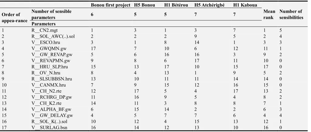
dominating the streamflow generation in the Bonou catchment. The chosen methodology for calibration was SUFI-2. So GSA was performed after each 500 simulations’ iteration. But considering the fact that it was the fourth iteration parameters values that were retained for calibration, its sensibility analysis was the most important. So, using the fourth iteration GSA for the five final projects, we derive the results present in Table 12 which gives the rank of their sensibility in projects and the number of sensibilities.

Table 12. Statistics of fourth iteration SUFI2 GSA for the sensible parameters ranking.

Bonou first project H5 Bonou H1 Bétérou H5 Atchérigbé H1 Kaboua Mean rank

Number of sensibilities Order of

appea-rance

Number of sensible

parameters 6 5 5 7 7

Parameters

1 R__CN2.mgt 1 3 1 3 7 1 5

2 R__SOL_AWC(..).sol 2 2 2 9 5 2 4

3 V__ESCO.hru 3 1 8 14 1 3 3

4 V__GWQMN.gw 17 7 10 6 12 11 1

5 V__GW_REVAP.gw 5 6 16 16 3 9 2

6 V__REVAPMN.gw 9 8 6 17 11 10 0

7 R__HRU_SLP.hru 15 13 17 10 15 17 0

8 R__OV_N.hru 8 4 13 1 9 5 2

9 R__SLSUBBSN.hru 13 10 11 11 14 14 0

10 V__CANMX.hru 7 9 15 12 16 15 0

11 V__CH_N2.rte 12 17 5 4 17 13 2

12 V__RCHRG_DP.gw 11 16 9 5 4 8 2

13 V__CH_K2.rte 14 11 3 8 8 7 1

14 V__ALPHA_BF.gw 6 15 14 2 2 6 3

15 V__GW_DELAY.gw 4 5 7 7 6 4 4

16 R__SOL_K(..).sol 10 12 4 15 13 12 1

17 V__SURLAG.bsn 16 14 12 13 10 16 0

The three most sensitive parameters (CN2, SOL_AWC, and ESCO) are directly related to the peak flows runoff, reflecting therefore the easy capacity of the model to simulate downflows and the dynamics in Ouémé river basins. One can notice here the dominance of the surface runoff on the streamflow generation in the Ouémé river catchment. Also, here the five additive parameters were not so good positioned though (CH_N2) got two times sensible, in Bétérou and Atchérigbé project which means that its sensibility in the large Bonou scale basin disappears by comparing to other parameters.

3.6. Model Predictive Uncertainty

Generally, model uncertainties are due to: (i) conceptual simplifications (e.g., SCS curve number method for flow partitioning), (ii) processes occurring in the watershed but not included in the program (e.g., wind erosion, wetland processes), (iii) processes that are included in the program, but their occurrences in the watershed are unknown to the modeler or unaccountable because of data limitation (e.g., dams and reservoirs, water transfers, farm management affecting water

quality), and (iv) input data quality. In large watershed applications, one expects to have all these forms of uncertainties, which explains some of the large prediction errors. In SUFI-2, parameter uncertainty accounts for all sources of uncertainty, e.g., input uncertainty, conceptual model uncertainty, and parameter uncertainty, because disaggregation of the error into its source components is difficult, particularly in cases common to hydrology where the model is nonlinear and different sources of error may interact to produce the measured deviation [77].

SWAT-CUP produces output results at each station as 95PPU as well as showing the best fit (e.g., the simulation run with the best objective function value), but for simplicity and clarity of presentation we only show the calibration/validation results for the Bonou basin, the individual sub basins and the final retained hypothesis simulation and report the overall statistics. The tables 13, 14 and 15 show the uncertainty results at all time steps for first Bonou project and internal outlets results, the individual sub basins in comparison, the final most accepted hypothesis results for Bonou, Bétérou, Atchérigbé and Kaboua.

Table 13. Predictive Uncertainty indices of Ouémé River SWAT model at Bonou gauging discharge station and its internal subbasins’ gauging stations.

Time Step Criterion Calibration (1982 - 1996)

Bonou Atchérigbé Ahlan Kaboua Savè Bétérou

Daily p-factor 0.73 0.46 0.77 0.61 0.49 0.52

r-factor 0.99 0.6 1.17 0.96 0.76 0.91

Monthly p-factor 0.54 0.33 0.58 0.43 0.33 0.32

Time Step Criterion Validation (1997 - 2010)

Bonou Atchérigbé Ahlan Kaboua Savè Bétérou

Daily p-factor 0.6 0.33 0.6 0.32 0.39 0.32

r-factor 0.52 0.51 0.45 0.43 0.39 0.47

Monthly p-factor 0.59 0.32 0.58 0.34 0.36 0.29

r-factor 0.8 0.64 0.66 0.72 0.51 0.58

Table 14. Predictive Uncertainty indices of Ouémé River SWAT model at Bétérou, Kaboua and Atchérigbé discharge gauging stations individually.

Time Step Criterion Calibration (1982 - 1996) Validation (1997 - 2010)

Bétérou Kaboua Atchérigbé Bétérou Kaboua Atchérigbé

Daily p-factor 0.39 0.46 0.38 0.37 0.28 0.2

r-factor 0.7 0.72 0.56 0.48 0.3 0.42

Monthly p-factor 0.31 0.51 0.42 0.38 0.32 0.28

r-factor 0.86 0.82 0.95 0.74 0.38 0.52

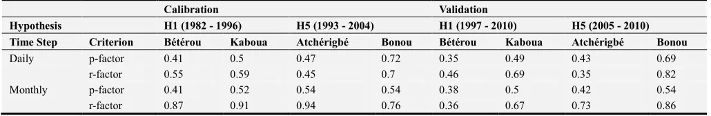
Table 15. Predictive Uncertainty indices of the best hypothesis Ouémé River SWAT model at Bonou, Kaboua, Atchérigbé and Bétérou discharge gauging stations individually.

Calibration Validation

Hypothesis H1 (1982 - 1996) H5 (1993 - 2004) H1 (1997 - 2010) H5 (2005 - 2010) Time Step Criterion Bétérou Kaboua Atchérigbé Bonou Bétérou Kaboua Atchérigbé Bonou

Daily p-factor 0.41 0.5 0.47 0.72 0.35 0.49 0.43 0.69

r-factor 0.55 0.59 0.45 0.7 0.46 0.69 0.35 0.82

Monthly p-factor 0.41 0.52 0.54 0.54 0.38 0.5 0.42 0.54

r-factor 0.87 0.91 0.94 0.76 0.36 0.67 0.73 0.86

The importance of both criteria appears to validate the range of parameters chosen. The r-factor is always less than 1.5 and most is less than 1; which is satisfied. The analysis lies then on the p-factor values. The Table 13 clearly shows that SWAT reproduces well the phenomenon happen to generate discharge using this parameters at the main outlet Bonou as for daily or monthly step. At internal outlet stage, the parameters range was well found for all subbasins except Atchérigbé for daily calibration. Savè and Bétérou results were acceptable. At monthly time step, only at Bonou and Ahlan, there were satisfied results which means that p-factor needs to be higher for daily calibration to facilitate interesting results at monthly time step because all the p-factors decrease while r-factor increase. For validation results too, only Bonou and Ahlan which outlet is not far from Bonou, gives good results. Parameters used and their range become less sensitive at individual internal basin scale and the simulation results appoint this deduction.

At internal basin scale project herein, one can notice that uncertainty band is very small while percentage is few. The results were not so good. But by comparing to their correspondent at internal stage using Bonou project, the band at individual project was larger while the percentage higher. It doesn’t help to conclude something.

For retained hypothesis uncertainty analysis results, Bonou and Kaboua were acceptable even if one knows Kaboua performance weren’t so satisfied. Simulation of the sub basin of Atchérigbé, although visually very good, suffers from a small lag in the simulation, which could not be corrected by the parameters listed in Table 2. This could have been caused by a small shift in the observed rainfall input governing this outlet in SWAT.

4. Discussion

In a real interest to assess the performance of a non lumped hydrological model, the SWAT model was chosen and applied on the Ouémé Rvier catchment at Bonou outlet. It is calibrated and validated on this large area at long time period the model at multiple sites on daily and monthly time steps by using measured climate data. The results were not so satisfactory on this long time period and with input discharge data used in calibration and validation. Therefore, analysis and hypotheses have been emitted to try to decrease at possible, some data errors which could deteriorate the model performance. Hypothesis H5 where data used are observed discharge data as got with no completion for missing values and where the simulation time period was 1993-2010, was retained. There was no statistically significant difference in model performance among time intervals. Using guidelines given in [66], the overall performance of the SWAT model in terms of NSE and R2 can be judged as very good, especially considering limited data conditions in the studied area. On a monthly basis, it is obtained at the Bonou outlet a NSE value equal to 0.90 for the calibration period (0.67 for the validation period). These results are greater than the ones obtained by [27], and [24] at the same outlet for calibration. Indeed, [27] reported a negative NSE (between 1 and 0) for the monthly calibration and a value ranging between 0 and 0.7 for monthly validation, while [24] obtained a NSE between 0 and 0.70 for both monthly calibration and validation.

72% of observed discharge data (54% for monthly calibration) in a narrow uncertainty band. These results are close to the results of [24] who estimated the observed discharge data bracketed by the 95PPU between 60% and 80% for monthly calibration (40% and 60% for monthly validation).

On the other hand, results showed that transferring the model parameters from the catchment outlet (Bonou) to the internal gauging stations performs reasonably well only in the case of similarity between donor and target catchments. The case of catchments controlled by Ahlan and Bonou gives a clear example of such physical proximity where precipitation, soil and land use vary smoothly between both catchments. However, it really does not perform well for the upstream internal gauging stations that account for tributaries of Ouéme River (Atchérigbé, Kaboua). According to K. Abbaspour discussions on his results on large scale basin internal outlets [60], the study results even for internal outlets were well simulated though. There is so much dissimilarity between donor and target catchments. The SWAT model parameters determined at these outlets could not reproduce well the measured discharge at Atchérigbé mainly due to more significant spatial dissimilarities.

Moreover, it has been demonstrated that the individual calibration at sub-catchment scale has led to a narrower uncertainty band and more observed discharge data enclosed in it, which is the sought adequate balance between the two indices. These results showed the importance of the calibration of hydrological models at finer spatial scale to ensure that predominant processes in each sub-catchment are captured, and this is particularly relevant in case of large-area global catchments. Concerning the effect of temporal scale, it demonstrated that the validation period is characterized by less predictive uncertainty as opposed to the calibration period. One explanation that can be given is the fact that last recent years (2005-2010, 2002-2010, 1997-2010) used in validation even in calibration constitutes a more humid period than olders (1982-1996, 1982-2001, 1993-2004) and is characterized, therefore, by less variability in precipitation. In contrast, when moving from daily to monthly calibration, the uncertainty of the model, in terms of uncertainty band width, increased. This could be attributed to the cumulative effect of uncertainty in daily discharge data used to compute monthly discharge, resulting therefore in larger monthly uncertainty. Overall, due to decreasing prediction uncertainty with decreasing spatial and temporal scales, it is germane to develop on the basin a more efficient system of hydro-meteorological data collection to account for spatial and temporal variabilities in hydro-meteorological systems prevailing in the region, especially under changing climate and land use conditions.

According to spatial performance, the results of different calibration and validation hypotheses showed varying predictive abilities of the SWAT model through scales. Firstly, it can be derived from these findings that model performance in terms of NSE and R2 was higher on the watershed-wide level than on the sub-watershed level. However, this could be attributed to compensation between positive and negative

errors of processes occurring at a larger scale [78, 79]. This suggests that calibrating a model only at the basin outlet leads to an over confidence in its performance than at the sub-basin scale. Secondly, individual calibration and validation of sub catchment were not as interesting as expected when realized on individual tributaries outlets. These results have an important role to play in the calibration and validation approaches of large-area watershed models and constitutes a first step to model parameter regionalization for prediction in ungauged basins.

This study is a step in that long-term direction, where an integrated water management tool would be developed and validated spatially on the Bonou catchment, which allows investigation of future effects of land use and climate change scenarios on water resources.

5. Conclusions

In this study, the performance of the widely-used SWAT model was evaluated on the Ouémé River at Bonou outlet catchment using both split-sample and split-location calibration and validation techniques on daily and monthly time step. The model was calibrated at the Bonou outlet and at five internal stations. Freely available global data and daily observed climate and discharge data were used as inputs for model simulation. Calibration, validation, uncertainty, and sensitivity analyses were performed with SUFI-2 within SWAT-CUP. Both graphical and statistical techniques were used for hydrologic calibration results evaluation.

Finally, it is noticed that at internal outlet sub-catchments, the long period 1982-2010 could not be accepted for validate the SWAT capacity to simulate discharge. However, a real good model is that one which could simulate discharge in all rainfall regimes even for dry and wet years. Another conclusion to lean on is this unavailability to get good performance in after 2000’ year’s simulation even in calibration and validation. It underlines the problem of parameters equifinality.

The results showed a good SWAT model performance to predict daily, as well as monthly discharge at Bonou with acceptable predictive uncertainty despite the poor data density and the high gradient of climate and land use characterizing the study catchment. However, the daily calibration resulted in less predictive uncertainty than the monthly calibration. Sub-catchment calibration induced an increase of model performance at intermediate gauging stations, as well as a decrease of total uncertainty. The GSA revealed the predominance of surface and subsurface processes in the streamflow generation of the Ouémé River catchment.

Overall, this study has shown the validity of the SWAT model for representing globally hydrological processes of a large-scale Soudano-Sahelian catchment in West Africa. Given the high spatial variability of climate, soil, and land use characterizing the catchment, additional calibration is however needed at sub-catchment level to ensure that predominant processes are captured in each sub-catchment.