A New Entropic Riemann Solver of Conservation Law of Mixed Type Including Ziti’s δ-Method with some Experimental Tests

(1)

http://www.sciencepublishinggroup.com/j/acm doi: 10.11648/j.acm.20170605.12

ISSN: 2328-5605 (Print); ISSN: 2328-5613 (Online)

A New Entropic Riemann Solver of Conservation Law of

Mixed Type Including Ziti’s δ-Method with Some

Experimental Tests

Larbi Bsiss, Cherif Ziti

Department of Mathematics, University Moulay Ismail, Meknes, Morocco

Email address:

[email protected] (L. Bsiss), [email protected] (C. Ziti)

*_{Corresponding author}

To cite this article:

Larbi Bsiss, Cherif Ziti. A New Entropic Riemann Solver of Conservation Law of Mixed Type Including Ziti’s δ-Method with Some Experimental Tests. Applied and Computational Mathematics. Vol. 6, No. 5, 2017, pp. 222-232. doi: 10.11648/j.acm.20170605.12 Received: June 30, 2017; Accepted: July 11, 2017; Published: September 26, 2017

Abstract

: Many problems in fluid mechanics and material sciences deal with liquid-vapour flows. In these flows, the ideal gas assumption is not accurate and the van der Waals equation of state is usually used. This equation of state is non-convex and causes the solution domain to have two hyperbolic regions separated by an elliptic region. Therefore, the governing equations of these flows have a mixed elliptic-hyperbolic nature. Numerical oscillations usually appear with standard finite-difference space discretization schemes, and they persist when the order of accuracy of the semi-discrete scheme is increased. In this study, we propose to use a new method called δ-ziti’s method for solving the governing equations. This method gives a new class of semi discrete, high-order scheme which are entropy conservative if the viscosity term is neglected. We implement a high resolution scheme for our mixed type problems that select the same viscosity solution as the Lax Friederich scheme with higher resolution. Several tests have been carried out to compare our results with those of [6] [9] [16], in the same situations, we obtained the same results but faster thanks to the CFL condition which reaches 0.8 and the simplicity of the method. We consider three types of pressure in these tests: Cubic, Van der Waals and linear in pieces. The comparison proved that the δ-ziti's method respects the generalized Liu entropy conditions, e.g. the existence of a viscous profile.

Keywords:

Hyperbolic, Van Der Waals, δ-ziti’s Method, System Mixed Type, The Lax-Friedrichs Scheme, Shock Wave, Rarefaction Wave, Viscous Profile

1. Introduction

The dynamics of compressible fluids undergoing liquid-solid or vapor-liquid phase transformations can be modeled by the standard balance laws (mass, momentum) supplemented with a nonconvex equation of state, such as the one introduced by van der Waals. Restricting attention to a model of two conservation laws (the temperature being, formally, kept constant), one knows that, above some (critical) temperature this model is hyperbolic but not globally genuinely nonlinear (the pressure is a decreasing but not a globally convex function of the specific volume); however, below the critical temperature, the model is a mixed (hyperbolic-elliptic) system of conservation laws (the pressure is decreasing except on some bounded interval).

The one-dimensional isothermal motion of a compressible elastic fluid or solid can be described in lagrangian coordinates by the coupled system:

, − , = 0; ∈ , ∈ 0, , , + , = 0; ∈ , ∈ 0, , (1)

(2)

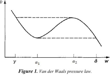
Figure 1. Van der Waals pressure law.

For convenience p will be globally defined, smooth, with

p w < 0; !" < α$ or w > α(

< 0; !" )$< < )(

)$ > 0, )( < 0

This type of constitutive relation is usually associated with a van der Waals fluid where

=_,-.*+ −_,/0 (2)

where c, d, T are numerical constants and where the temperature T>0 is fixed.

First to begin at the case where the van der Waals pressure can be well approximated by the cubic equation

= + 1 − − 2₍₃₎

where c and d are numerical constants.

Here we need nothing so specific as the van der Waals constitutive relation though our results will strongly depend at times on the global behavior of p as | | → ∞.

The reason for this non-standard choice of p is that it serves as a prototype problem for the dynamics of materials exhibiting changes of phase. For example in a van der Waals fluid the states < )_$ are viewed as liquid while states with

> )( are viewed as vapor. Because p is not monotone, liquid and vapor phases may co-exist.

The evolution of the first and second equations of (1) will be governed by initial data. Here we pose piecewise constant data

67 = 86

-_{!" < 0}

69_{!" > 0,} (4)

which makes (1) and (4) into a mixed hyperbolic-elliptic Riemann initial value problem.

Solutions of such systems of nonlinear PDEs are generally discontinuous and exhibit several distinct types of propagating waves:

a. Compressive shock waves satisfying the standard Lax or Liu entropy criteria;

b.Rarefaction waves, which are smooth and self-similar solutions;

c. Supersonic phase boundaries, which propagate faster than the characteristic speed;

d.In the mixed type case, stationary phase boundaries.

Until recently the Riemann problem (for which the initial data is a single step function) was solved allowing only stationary and supersonic phase boundaries plus standard classical waves [10, 20]. Recently, after the works by James [15], Truskinovsky [25, 26], Slemrod [23], Abeyaratne and Knowles [1, 2], Le Floch [17-19], Shearer [14, 21], and Hayes and LeFloch [11-13], it became clear that nonstationary, subsonic phase interfaces (in the hyperbolic-elliptic regime) and nonclassical shock waves (in the hyperbolic, but not genuinely nonlinear regime) should be included when solving the Riemann problem.

Indeed, such waves are admissible in the sense that they do arise in viscosity-capillarity limits of the system.

Subsonic phase boundaries and nonclassical shocks have a special flavor: they are not uniquely characterized by the standard Rankine-Hugoniot relations and their unique selection requires as additional jump relation called a kinetic relation. Recall that there is indeed no universal selection criterion for propagating phase boundaries. The basic reason is that such waves are under compressive, in the sense that-compared with compressive shocks-fewer characteristics are impinging on the discontinuity.

The numerical approximation of the model under consideration was initiated by Slemrod and followers [3, 8, 16, 22, 24]. Computing kinetic relations to characterize under compressive waves such as no classical shocks and subsonic phase boundaries was first tackled by Hayes and LeFloch [13], who identified the basic issues arising numerically. The present paper is a natural extension of [13].

The resolution of the Riemann problem is still a very complicated task. For any Cauchy problem, the numerical schemes that lead to an admissible solution (entropy solution) are based on the exact solution of the Riemann problem which further complicates the situation. Other schemes require the existence of a viscous profile.

In this work, a new scheme called zitis δ-scheme [4] is applied. We recall that our scheme has yielded impressive results especially for hyperbolic problems [5].

For the mixed system (1) we take the same scheme δ-ziti's scheme and we organize our work as following:

In Section 2, we posed the problem, in Sections 3 and 4, we applied our scheme to the system (1) with a pressure p (w) of the form (2), (3) and at the end of the form (27).

The results were compared with [6], with [9] and [16]. They are impressive.

2. Problem Position

In one dimension, the equation of isothermal motion for a compressible fluid in Langragian coordinates takes the form:

: ; < ;

= , − , = 0; ∈ , ∈ 0, , , + , = 0; ∈ , ∈ 0, ,

> ,7 ?>@ ? A>_>BF CD E7_{CD G7 ; ∈ H,I ,} JK

JLH, ?JKJLI, ?7 ; ∈ 7,+M

, (5)

(3)

the initial data function, w is the specific volume, u is the velocity, and p is the pressure, U-=(w-, u-)T and U+=(w+, u+)T.

The system (5) can be writing under a non-conservative form:

N

6 , O 6 6 , 0; ∈ , ∈ 0, ,

> ,7 ?>@ ? A>_>BF CD E7_{CD G7 ; ∈ H,I ,} JK

JLH, ?JKJLI, ?7 ; ∈ 7,+M

, (6)

where,

O 6 P 0 1_0R

is a constant matrix of 2 order.

Notice that the eigenvalues of A (U) are ST , which become real in the hyperbolic region and complex in the elliptic region.

3. Numerical Approximation of Solution

In this section we describe how to apply the δ-ziti's method to the system (5).

We take an uniform mesh of the interval [a, b] with the step U I-H_V where m is an integer such _$ , _V9$ , xi=a+(i-1)h, for i=1, m+1.

The δ-ziti's method is based on the Galerkin method: First, we approximate the weak solution U(x, t) of (1) by:

, W ∑V9$D?$ )DYD (7)

and

, W Z [D

V9$

D?$

YD

where, Y_D isthe orthonormal family defined as follow:

YD _{_\]}\]^_^ _{_} (8)

where, `Ybca is the orthogonal family which satisfies the following recurrence relation:

N

Yd$ e$ ∀ ∈ $, V9$

YdD eD gD-$YdD-$ ∀ ∈ $, V9$ ; ! 2, … , j 1

Uklm, gD-$ En_{_\]}^,n^BoG

^Bo_0

(9)

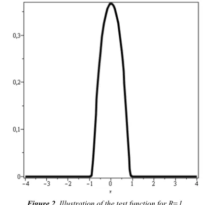
ea is obtained from the test function (figure 2):

Φ exp s 0_-*$ 0t ; | | u

0 v Ukl !mk (10) where R is a positive constant, m is an integer such _$

and _V9$ .

Figure 2. Illustration of the test function for R=1.

As, the framework of the Galerkin method, we multiply the first and second equations of (1) by Y_a and integrating it over [a, b] we obtain:

w_HI , Ya w_HI , Ya 0

Now, we use the x y roots of Y_V9$ on the interval [a, b] l_a as points of meshing instead of the _a, And put l_V9$ _V9$ [4].

From [4] we have,

zI ,

H Ya W

la,

Ya la

w_HI , Ya W{L_\, |_}_|}_},

therefore,

w ∑_HI V9$D?$ )D YD Ya ~_\L_}|_|}_}, 0 (11)

w ∑_HI V9$D?$ [D YD Ya {L_\`, |_}_|}_}, c 0 (12)

By using the orthonormal property of the Y_D we obtain,

z Z )D

V9$

D?$ I

H YD Ya Z )D

V9$

D?$

z YD Ya

I

H )a

z Z [D

V9$

D?$ I

H YD Ya Z [D

V9$

D?$

z YD Ya

I

H [a

(4)

)a −~L_\_}|_|}_}, = 0 (13)

[a +{L_\, |},_}_|_} = 0 (14)

To approximate (13) and (14), we denote by:

a• the approximate value of the l_a,

)a• the approximate value of the )a a• the approximate value of the la,

[a• the approximate value of the [a

For example, if we take the center finite difference approximation which is second order accuracy:

la, ≈ la9$_l, − la-$, a9$− la-$

la, ≈ ` la9$_l, c − ` la-$, c a9$− la-$

then, for t=ndt,

la, . ≈ a9$

• ₋

a-$•

la9$− la-$

la, . ≈ a9$

• ₋

a-$•

la9$− la-$

From [4] we have,

la, = )a Ya la

la, = [a Ya la

and,

)a = _Yla, a la ≈

la9$, + la-$,

2. Ya la

[a = _Yla, a la ≈

la9$, + la-$,

2. Ya la

By taking the time semi discretization as following:

)a =)a •9$_{− )}

a•_{= .}

[a =[a •9$_{− [}

a•_{= .}

Therefore (13) and (14) become,

)a•9$=,}Fo • _9,

}Bo • (.\}|} + ga

~}Fo• -~}Bo•

\}|} ; x = 2, … , j, (15)

[a•9$=~}Fo • _9~

}Bo • (.\}|} − ga

{`,_}Fo• c-{`,_}Bo• c

\}|} ; x = 2, … , j, (16)

where, g_a=_| /

}Fo-|}Bo.

On the other hand, the initial data U0 can be approximated by,

7 ≈ Z_Y7 lD D lD V9$

D?$

YD

7 ≈ Z_Y7 lD D lD V9$

D?$

YD

therefore,

)a$=,_\@_}|_|}_} ; x = 1, … , j + 1 (17)

[a$=_\~@_}|_|}_} ; x = 1, … , j + 1 (18)

The Neumann conditions in (5) are approximated by,

: ; < ;

= $•9$= (•9$, $•9$= (•9$, V9$•9$ = V•9$, V9$ •9$ ₌ V •9$_, therefore, : ;; < ;;

= )$•9$ = ,0 •Fo \o |o

[$•9$= ~0 •Fo \o |o

)V9$•9$ = ,‚ •Fo \‚Fo|‚Fo

[V9$•9$ = ~‚ •Fo \‚Fo|‚Fo

(19)

By combining (15-19), we build an algorithm which enable to compute )_a• and [_a• at each level n (n ≥1) in accordance with the following scheme,

: ; ; ; ; < ; ; ; ;

=)a$=_\,@_}|_|}_} ; x = 1, … , j + 1,

[a$=_\~@_}|_|}_} ; x = 1, … , j + 1,

ƒ_}•Fo?„}Fo• F„}Bo•

0.…}`†}c -‡}ˆ}Fo• Bˆ}Bo •

…}`†}c ; a?(,…,V, ‰_}•Fo?ˆ}Fo• Fˆ}Bo_0.…}`†}c• 9‡}Šs„}Fo• tBŠs„}Bo_…}`†}c• t ; a?(,…,V,

ƒ_o•Fo_?„0•Fo

…o †o; ‰o•Fo?_{…o †o}ˆ0•Fo

)V9$•9$ = ,‚ •Fo

\‚Fo|‚Fo ; [V9$

•9$ ₌ ~‚•Fo \‚Fo|‚Fo

(20)

where, g_a =_| /

}Fo-|}Bo

4. Applications

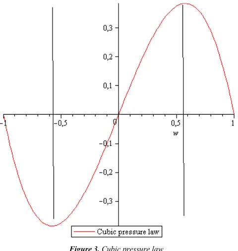
4.1. Cubic Pressure Law

(5)

Figure 3. Cubic pressure law.

4.1.1. Test 1 and Comparison with [16]

To compare our results, we take the same data as SHI JIN: c=0 and d=0. [16]

The δ-ziti's scheme (20) Applied to the Riemann problem:

6- _{= P} -= 0.7

- = −0.7R ; 6

9_{= P} 9= −0.327

9= −0.327R (21)

The system (1) change of type (hyperbolic-elliptic) following the sign of :

The elliptic region is the domain ∈ )_$; )₍ , the hyperbolic region is outside ∈ _-;)_$ ∪ )₍; ₉, figure 4. Where, )_$= −√2₂, and )₍=√2₂

Figure 4. Hyperbolic-elliptic region.

The ziti's δ-method gives the same results founded in [16], figure 5.

Figure 5. The numerical solutions of (1) obtained by ziti's δ-scheme (20) at t=2 with initial data (21).

New, we take the LeFlock data (22) to compare our results: c=4 and d=6. [6]

The δ-ziti's scheme (20) Applied to the following Riemann problem:

w x, 0 = Pw-= 3

w9= 5R; , 0 = P -= 0

9= 2R (22)

The system (1) change of type (hyperbolic-elliptic) with the sign of :

The elliptic region is the domain ∈ )_$; )₍ , the hyperbolic region is the domain ∈ _-;)_$ ∪ )₍; ₉ . Where, )_$= 4 −√2₂and )₍= 4 +√2₂

The δ-ziti's method gives the same results than founded in [6] figure 6.

(6)

Table 1. Set of selected tests in different regions.

Test number N

Left state U

-right state U+

IWW(*)

U-_{→ U}9 _Figure

1 (1; 0) “√3

3 , 0.5” R1 S2 figure 7

2 (1; 0.5) “√3

3 , 0.5” R1 S2 figure 8

3 (1; 0.5) “√3

3 , 0” R1 S2 figure 8

4 (1; -0.5) “√3

3 , 0.5” S1 R2 figure 10

5 (1;-0.5) “√3

3 , −0.1” S1 figure 11

6 s−√2

2, 0.5t (-0.7; 0) S1 R2 figure 12

7 (-0.6; 1) (-1; 0.5) S1 R2 figure 13

8 (-0.6; -0.4) (-1; -1) S1 R2 figure 14

9 (1; 0.5) (-1; 0.1) R1 DCR2 figure 15

10 (1; -0.5) (-1; 0.1) R1 DCR2 figure 16

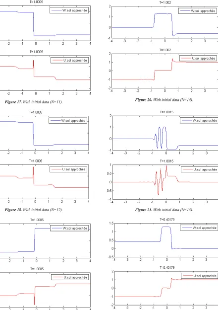
11 (1; 0.5) (-1; -0.1) R1 DCR2 figure 17

12 (1; -0.5) (-1; -1) R1 DCR2 figure 18

13 (-1; -1) (1; -0.5) R1 DCR2 figure 19

14 “√3

3 , −0.5” “−√33 , −0.5” S1 DCS2 figure 20

15 (0; 0) “− √3

3 , 0” SSSSR figure 21

16 (0.4; -1) (0; 1) S1 S2 figure 22

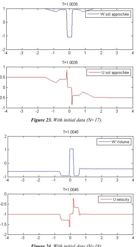
17 (1; 0.5) (1; -0.5) RRSSRR figure 23

18 (-0.6; -1) (-0.4; -1) SSSS figure 24

(*) IWW: The Intermediate Wave Way.

Where; Ri is the i-rarefaction, Sj is the j-shock and DC is the contact discontinuity.

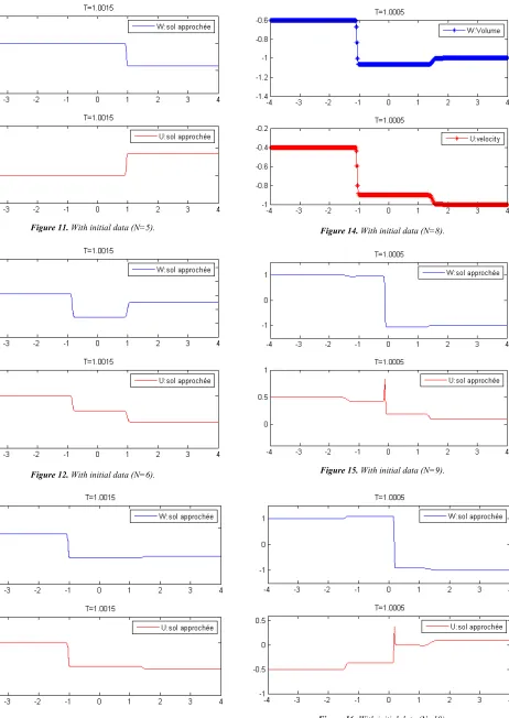
We present here the test given in the table 1: The are some numerical solutions of (1) obtained by δ-ziti's scheme (20) at t=1.

Figure 7. With initial data (N=1).

(7)

(8)

(9)

4.2. Van der Waals Pressure Law

In this section we deal with the well-known van der Waals equation of state, given by (2) presented in figure 25.

Figure 25. Van der Waals pressure law.

For the same data that given in [16], the δ-ziti's scheme (20) applied to the following Riemann problem:

w x, 0 = Pw-= 0.54

w9= 1.8517R; u x, 0 = Pu

-= 1

u9= 1 R (25)

where, a=0.9, =$_—, R=1 and T=1.

The elliptic region is the domain ∈ )_$; )₍ , the hyperbolic region is the domain

∈ -;)$ ∪ )(; 9 .

Where, )_$= 0.5749122774 and )₍= 1.0362512534 The δ-ziti's method gives the same results than founded in [16]. Figure 26.

Applying the δ-ziti's scheme (20) to the following Riemann problem:

, 0 = P -= 0.787

9= 1.33 R; , 0 = P

-= −2

9= 0 R (26)

where a=3, =$₂, u =š₂ and T=0.95.

The elliptic region is the domain ∈ )_$; )₍ , the hyperbolic region is the domain

∈ -;)$ ∪ )(; 9 .

Where, )_$= 0.684 and )₍= 1.2354

(10)

Figure 27. The numerical solutions of (1) obtained by ziti's δ-scheme (20) at t=3.2 with initial data (26).

4.3. Piecewise-Linear Equation of State

To compare our results, we take the same data as SHI JIN. We test the δ-ziti's scheme for a piecewise-linear equation of state:

= ›−3 + 10 !" 0.1 ≤ < 0.2, −20 !" < 0.1, −5 !" 0.2 ≤ (27)

In our numerical experiments we take the initial data:

, 0 = P -= 0.05

9 = 0.07 R; , 0 = P

-= 0

9 = 0.5 R (28)

The elliptic region is the domain ∈ )_$; )₍ , the hyperbolic region is the domain ∈ −∞; )_$ ∪ )₍; +∞

Where, )_$= 0.1 and )₍= 0.2

The δ-ziti's method gives the same results than founded in [16], figure 28.

Figure 28. The numerical solutions of (1) obtained by ziti's δ-scheme (20) at t=0.05 with initial data (28).

5. Conclusions

The application of δ-ziti’s method to the hyperbolic-elliptic mixed system has proven to be very robust, fast and efficient without using the exact solution of the Riemann problem. Its ability is to approach the entropy solution (physically admissible) of the system. The comparison with the exact solution or with the results of [6] [9] [16] showed that for the same Riemann problems, the δ-ziti’s scheme detects the same intermediate states in different phase positions.

The comparison with the exact solution showed the existence of the viscous profile [23].

We have enriched our investigation with other untreated tests in [6] [16] to complement the numerical study of our system.

The comparison of our numerical results with [6] [16] has shown us several advantages:

a. The stability condition CFL is near 0.8 and approaches 1, whereas that of [6] [16] for some cases the CFL is less than 0.25 and for other CFL is less than 0.5. b.The amelioration of the CFL saves time for advanced

previsions (less iteration to achieve the required time). c. In [16], small oscillations appear from a certain time in

order schemes and disappear in 2-order schemes. In our scheme, there are no oscillations.

d.In presence of shock waves, the scheme of [16] smooths the solution a little, giving the impression that it is a rarefaction wave; Contrary to the scheme of δ-ziti which makes the difference between the two waves. In conclusion, with scheme of δ-ziti, we were able to obtain the same results as those [6] [16]; the same intermediate states, the same waves and the same solution but with a simplicity, an incredible rapidity.

Acknowledgements

We warmly thank Shi Jin, P. G. Le Floch and Haitao Fan, because thanks to their numerical results we were able to test the ziti’s δ-method.

In addition, I would like to thank Marshall Slemrod for their works on mixed type problems.

References

[1] R. Abeyaratne and J. K. Knowles, “Kinetic relations and the propagation of phase boundaries in solids”, Arch Rational Mech. Anal. 114, 119 (1991).

[2] R. Abeyaratne and J. K. Knowles, “Implications of viscosity and strain gradient effects for the kinetics of propagating phase boundaries”, SIAM J. Appl. Math. 51, 1205 (1991).

(11)

[4] L. BSISS, C. ZITI, “A new numerical method for the integral approximation and solving the differential problems: Non-oscillating scheme, detecting the singularity in one and several dimensions”, J. Ponte, Vol. 73, Issue 2, pp. 126-172.

[5] L. BSISS, C. ZITI, “A new Approximation (ziti’s δ-scheme) of the Entropic (Admissible) Solution of the Hyperbolic Problems in One and Several Dimensions: Applications to Convection, Burgers, Gas Dynamics and Some Biological Problems”, Turkish Journal of Analysis and Number Theory. 2016, 4(4), 98-108.

[6] C. Chalons and P. G. Le Floch, “High-Order Entropy-Conservative and Kinetic Relations for van der Waals Fluids”, Journal of Computational Physics. (2001), 184-206.

[7] C. Chalons and P. G. LeFloch, “A fully discrete scheme for diffusive-dispersive conservation laws”, Numerische Math. (2001), to appear.

[8] B. Cockburn and H. Gau, “A model numerical scheme for the propagation of phase transitions in solids”, SIAM J. Sci. Comput. 17, 1092 (1996).

[9] H. T. Fan, “A limiting “viscosity” approach to the Riemann problem for materials exhibiting a change of phase II”, Arch. Rational Mech. Anal. (1992) 116, 317.

[10] H. Hattori, “The Riemann problem for a van der Waals fluid with the entropy rate admissibility criterion”, Arch. Rational Mech. Anal. 92, 247(1936).

[11] B. T. Hayes and P. G. Le Floch, “Nonclassical shocks and kinetic relationsrelations: Scalar conservation laws”, Arch Rational Mech. Anal. 139, 1 (1997).

[12] B. T. Hayes and P. G. Le Floch, “Nonclassical shocks and kinetic relations: Finite difference schemes”, SIAM J. Numer. Anal. 35, 2169 (1998).

[13] B. T. Hayes and P. G. Le Floch, “Nonclassical shocks and kinetic relations: Strictly hyperbolic systems”, SIAMJ. Math. Anal. 31, 941 (2000).

[14] D. Jacobs W. R. McKinney, and M. Shearer, “Traveling wave solutions of the modified Korteweg-de Vries Burgers equation”, J. Differential Equations 116, 448 (1995).

[15] R. D. James, “The propagation of phase boundaries in elastic bars”, Arch. Rational Mech. Anal. 73, 125 (1980).

[16] S. Jin, “Numerical integrations of systems of conservation laws of mixed type”, SIAM J. Appl. Math. 55, 1536 (1995). [17] P. G. Le Floch, “Propagating phase boundaries: Formulation

of the problem and existence via the Glimm scheme”, Arch. Rational Mech. Anal. 123, 153 (1993).

[18] P. G. Le Floch, “An introduction to nonclassical shocks of systems of conservation laws, in Proceedings of the International School on Theory and Numerics for Conservation Laws”, Freiburg Littenweiler (Germany), 20–24 October 1997, edited by D. Kr¨oner, M. Ohlberger, and C. Rohde, Lecture Notes in Computational Science and Engineering, (1998), p. 28.

[19] P. G. LeFloch, “Hyperbolic Systems of Conservation Laws: The Theory of Classical and Nonclassical Shock Waves”, E. T. H. Lecture Notes Series, 2001, to appear.

[20] M. Shearer, “the Riemann problem for a class of conservation laws of mixed type”, J. Differential Equations 46, 426 (1982). [21] M. Shearer and Y. Yang, “The Riemann problem for the p-system of conservation laws of mixed type with a cubic nonlinearity”, Proc. Roy. Soc. Edinburgh. 125A, 675 (1995). [22] C.-W. Shu, “A numerical method for systems of conservation

laws of mixed type admitting hyperbolic flux splitting”, J. Comput. Phys. 100, 424 (1992).

[23] M. Slemrod, “Admissibility criteria for propagating phase boundaries in a van der Waals fluid”, Arch. Rational Mech. Anal. 81, 301 (1983).

[24] M. Slemrod and J. E. Flaherty, “Numerical integration of a Riemann problem for a van der Waals fluid, in Phase Transformations”, edited by C. A. Elias and G. John (Elsevier, Amsterdam, 1986).

[25] L. Truskinovsky, “Dynamics of non-equilibrium phase boundaries in a heat conducting nonlinear elastic medium”, J. Appl. Math. Mech. 51, 777 (1987).