Towards Integrative Causal Analysis of Heterogeneous Data Sets and Studies

Towards Integrative Causal Analysis of

Heterogeneous Data Sets and Studies

Ioannis Tsamardinos∗ TSAMARD@ICS.FORTH.GR

Sofia Triantafillou∗ STRIANT@ICS.FORTH.GR

Vincenzo Lagani VLAGANI@ICS.FORTH.GR

Institute of Computer Science

Foundation for Research and Technology - Hellas (FORTH) N. Plastira 100 Vassilika Vouton

GR-700 13 Heraklion, Crete, Greece

Editor: Chris Meek

Abstract

We present methods able to predict the presence and strength of conditional and unconditional dependencies (correlations) between two variables Y and Z never jointly measured on the same samples, based on multiple data sets measuring a set of common variables. The algorithms are specializations of prior work on learning causal structures from overlapping variable sets. This problem has also been addressed in the field of statistical matching. The proposed methods are applied to a wide range of domains and are shown to accurately predict the presence of thousands of dependencies. Compared against prototypical statistical matching algorithms and within the scope of our experiments, the proposed algorithms make predictions that are better correlated with the sample estimates of the unknown parameters on test data ; this is particularly the case when the number of commonly measured variables is low.

The enabling idea behind the methods is to induce one or all causal models that are simultane-ously consistent with (fit) all available data sets and prior knowledge and reason with them. This allows constraints stemming from causal assumptions (e.g., Causal Markov Condition, Faithful-ness) to propagate. Several methods have been developed based on this idea, for which we propose the unifying name Integrative Causal Analysis (INCA). A contrived example is presented demon-strating the theoretical potential to develop more general methods for co-analyzing heterogeneous data sets. The computational experiments with the novel methods provide evidence that causally-inspired assumptions such as Faithfulness often hold to a good degree of approximation in many real systems and could be exploited for statistical inference. Code, scripts, and data are available at www.mensxmachina.org.

Keywords: integrative causal analysis, causal discovery, Bayesian networks, maximal ancestral graphs, structural equation models, causality, statistical matching, data fusion

1. Introduction

In several domains it is often the case that several data sets (studies) may be available related to a specific analysis question. Meta-analysis methods attempt to collect, evaluate and combine the results of several studies regarding a single hypothesis. However, studies may be heterogeneous in

several aspects, and thus not amenable to standard meta-analysis techniques. For example, different studies may be measuring different sets of variables or under different experimental conditions.

One approach to allow the co-analysis of heterogeneous data sets in the context of prior knowl-edge is to try to induce one or all causal models that are simultaneously consistent with all available data sets and pieces of knowledge. Subsequently, one can reason with this set of consistent models. We have named this approach Integrative Causal Analysis (INCA).

The use of causal models may allow additional inferences than what is possible with non-causal models. This is because the former employ additional assumptions connecting the concept of causality with observable and estimable quantities such as conditional independencies and depen-dencies. These assumptions further constrain the space of consistent models and may lead to new inferences. Two of the most common causal assumptions in the literature are the Causal Markov Condition and the Faithfulness Condition (Spirtes et al., 2001); intuitively, these conditions assume that the observed dependencies and independencies in the data are due to the causal structure of the observed system and not due to accidental properties of the distribution parameters (Spirtes et al., 2001). Another interpretation of these conditions is that the set of independencies is stable to small perturbations of the joint distribution (Pearl, 2000) of the data.

The idea of inducing causal models from several data sets has already appeared in several prior works. Methods for inducing causal models from samples measured under different experimental conditions are described in Cooper and Yoo (1999), Tian and Pearl (2001), Claassen and Heskes (2010), Eberhardt (2008); Eberhardt et al. (2010) and Hyttinen et al. (2011, 2010). Other methods deal with the co-analysis of data sets defined over different variable sets (Tillman et al., 2008; Triantafillou et al., 2010; Tillman and Spirtes, 2011). In Tillman (2009) and Tsamardinos and Borboudakis (2010) approaches that induce causal models from data sets defined over semantically similar variables (e.g., a dichotomous variable for Smoking in one data set and a continuous variable for Cigarettes-Per-Day in a second) are explored. Methods for inducing causal models in the context of prior knowledge also exist (Angelopoulos and Cussens, 2008; Borboudakis et al., 2011; Meek, 1995; Werhli and Husmeier, 2007; O’Donnell et al., 2006). INCA as a unifying common theme was first presented in Tsamardinos and Triantafillou (2009) where a mathematical formulation is given of the co-analysis of data sets that are heterogeneous in several of the above aspects. In Section 3, we present a contrived example demonstrating the theoretical potential to develop such general methods.

In this paper, we focus on the problem of analyzing data sets defined over different variable sets, as proof-of-concept of the main idea. We develop methods that could be seen as special cases of general algorithms that have appeared for this problem (Tillman et al., 2008; Triantafillou et al., 2010; Tillman and Spirtes, 2011). The methods are able to predict the presence and strength of conditional and unconditional dependencies (correlations) between two variables Y and Z never jointly measured on the same samples, based on multiple data sets measuring a set of common variables.

To evaluate the methods we simulate the above situation in a way that it becomes testable: a single data set is partitioned to three data sets that do not share samples. A different set of variables is excluded from each of the first two data sets, while the third is hold out for testing. Based on the first two data sets the algorithms predict certain pairs of the excluded variables should be dependent. These are then tested in the third test set containing all variables.

ran-dom. The methods also successfully predict certain conditional dependencies between pairs of

variables Y,Z never measured together in a study. In addition, when linear causal relations and

Gaussian error terms are assumed, the algorithms successfully predict the strength of the linear cor-relation between Y and Z. The latter observation is an example where the INCA approach can give rise to algorithms that provide quantitative inferences (strength of dependence), and are not limited to qualitative inferences (e.g., presence of dependencies).

Inferring the correlation between Y and Z in the above setting has also been addressed by statis-tical matching algorithms (D’Orazio et al., 2006), often found under the name of data fusion in Eu-rope. Statistical matching algorithms make predictions based on parametric distributional assump-tions, instead of causally-inspired assumptions. We have implemented two prototypical statistical matching algorithms and performed a comparative evaluation. Within the scope of our experiments, the proposed algorithms make predictions that are better correlated with the sample estimates of the unknown parameters on test data; this is particularly the case when the number of commonly measured variables is low. In addition, the proposed algorithms make predictions in cases where some statistical matching procedures fail to do so and vice versa, and thus, the two approaches can be considered complementary in this respect.

There are several philosophical and practical implications of the above results. First, the results provide ample statistical evidence that some of the typical assumptions employed in causal modeling hold abundantly (at least to a good level of approximation) in a wide range of domains and lead to accurate inferences. To obtain the results the causal semantics are not employed per se, that is, we do not predict the effects of experiments and manipulations. In other words, one could view the assumptions made by the causal models as constraints or priors on probability distributions encountered in Nature without any reference to causal semantics.

Second, the results point to the utility and potential impact of the approach: co-analysis pro-vides novel inferences as a norm, not only in contrived toy problems or rare situations. Future INCA-based algorithms that are able to handle all sorts of heterogeneous data sets that vary in terms of experimental conditions, study design and sampling methodology (e.g., case-control vs. i.i.d. sampling, cross-sectional vs. temporal measurements) could potentially one day enable the auto-mated large-scale integrative analysis of a large part of available data and knowledge to construct causal models.

The rest of this document is organized as follows: Section 2 briefly presents background on causal modeling with Maximal Ancestral Graphs. Section 3 discusses the scope and vision of the INCA approach. Section 4 presents the example scenario employed in all evaluations. Section 5 formalizes the problem of co-analysis of data sets measuring different quantities. Sections 6 and 7 present the algorithms and their comparative evaluation for predicting unconditional and conditional dependencies respectively, between variables not jointly measured. Section 8 extends the theory to devise an algorithm that can also predict the strength of the dependence. Section 9 presents the statistical matching theory and comparative evaluation. The paper concludes with Section 10 and 11 discussing the related work and the paper in general.

2. Modeling Causality with Maximal Ancestral Graphs

de-veloped without any reference to their causal semantics; nevertheless, we also briefly discuss their causal interpretation.

MAGs can be viewed as a generalization of Causal Bayesian Networks. The causal semantics

of an edge A→B imply that A is probabilistically causing B, that is, an (appropriate) manipulation

of A results in a change of the distribution of B. Edges A↔B imply that A and B are associated

but neither A causes B nor vice-versa. Under certain conditions, the independencies implied by the model are given by a graphical criterion called m-separation, defined below. A desired property of MAGs is that they are closed under marginalization: the marginal of a MAG is a MAG. MAGs can also represent the presence of selection bias, but this is out of the scope of the present paper. We present the key theory of MAGs, introduced in Richardson and Spirtes (2002).

A path in a graph

G

= (V,E)is a sequence of distinct verticeshV0,V1, . . . ,Vniall of them in O

s.t for 0≤i<n, Vi and Vi+1are adjacent in

G

. A path from V0to Vnis directed if for 0≤i<n, Vi

is a parent Vi+1. X is called an ancestor of Y and Y a descendent of X if X=Y or there is a directed

path from X to Y in

G

. AnG(X)is used to denote the set of ancestors of node X in

G

. A directed

cycle in

G

occurs when X→Y ∈E and Y ∈AnG(X). An almost directed cycle in

G

occurs when

X↔Y ∈E and Y∈AnG(X).

Definition 1 (Mixed and Ancestral Graph) A graph is mixed if all of its edges are either directed

or bi-directed. A mixed graph is ancestral if the graph does not contain any directed or almost directed cycles.

Given a path p=hV0,V1, . . . ,Vni, node Vi, i∈1,2, . . . ,n is a collider on p if both edges incident to Vi

have an arrowhead towards Vi. We also say that triple(Vi−1,Vi,Vi+1)forms a collider. Otherwise Vi

is called a non-collider on p. The criterion of m-separation leads to a graphical way of determining the probabilistic properties stemming from the causal semantics of the graph:

Definition 2 (m-connection, m-separation) In a mixed graph

G

= (E,V), a path p between A and

B is m-connecting relative to (condition to) a set of vertices Z , Z⊆V\ {A,B}if

1. Every non-collider on p is not a member of Z.

2. Every collider on the path is an ancestor of some member of Z.

A and B are said to be m-separated by Z if there is no m-connecting path between A and B relative to

Z. Otherwise, we say they are m-connected given Z. We denote the m-separation of A and B given Z as MSep(A; B|Z). Non-empty sets A and B are m-separated given Z (symb. MSep(A; B|Z)) if for

every A∈A and every B∈B A and B are m-separated given Z. (A, B and Z are disjoint). We also

define the set of all m-separations as

J

m(

G

):

J

m(

G

)≡ {hX,Y|Zi,s.t. MSep(X; Y|Z)and X,Y,Z⊆O}.

We also define the set

J

of all conditional independencies X⊥⊥Y|Z, where X, Y and Z are

disjoint sets of variables, in the joint distribution of

P

of O:

J

(

P

)≡ {hX,Y|Z|i,s.t.,X⊥⊥Y|Z and X,Y,Z⊆O}.

The set

J

(

P

)is also called the independence model of

P

. The m-separation criterion is meant

Definition 3 (Faithfulness) We call a distribution

P

over a set of variables O faithful to a graph

G

, and vice versa, iff:

J

(

P

) =

J

m(

G

).

A graph is faithful iff there exists a distribution faithful to it. When the above equation holds, we say the Faithfulness Condition holds for the graph and the distribution.

When the faithfulness condition holds, every m-separation present in

G

corresponds to a

condi-tional independence in

J

(

P

)and vice-versa. The following definition describes a subset of

ances-tral graphs in which every missing edge (non-adjacency) corresponds to at least one conditional independence:

Definition 4 (Maximal Ancestral Graph, MAG) An ancestral graph

G

is called maximal if for

every pair of non-adjacent vertices (X,Y), there is a (possibly empty) set Z, X,Y ∈/Z such that

hX,Y|Zi ∈

J

(

G

).

Every ancestral graph can be transformed into a unique equivalent MAG (i.e., with the same independence model) with the possible addition of bi-directed edges. We denote the marginal of a

distribution

P

over a set of variables V\L L as

P

[L, and the independence model stemming from

the marginalized distribution as

J

(

P

)[L, that is,

J

(

P

[L) =

J

(

P

)[L≡ {hX,Y|Zi ∈

J

(

P

):(X∪Y∪Z)∩L=/0}.

Equivalently, we define the set of m-separations of

G

restricted on the marginal variables as:

J

m(

G

)[L≡ {hX,Y|Zi ∈

J

m(

G

):(X∪Y∪Z)∩L=/0}.

A simple graphical transformation for a MAG

G

faithful to a distribution

P

with independence

model

J

(

P

) exists that provides a unique MAG

G

[L that represents the causal ancestral relations

and the independence model

J

(

P

)[Lafter marginalizing out variables in L. Formally,

Definition 5 (Marginalized Graph

G

[L) Graph

G

[L has vertex set V\L, and edges defined as

follows: If X,Y are s.t. ,∀Z⊆V\(L∪ {X,Y}),hX,Y|Zi∈/

J

(

G

)and

X∈/AnG(Y);Y ∈/AnG(X)

X∈AnG(Y);Y ∈/AnG(X)

X∈/AnG(Y);Y ∈AnG(X)

then

X↔Y

X→Y

X←Y

in

G

[L.

We will call

G

[Lthe marginalized graph

G

over L.

The following result has been proved in Richardson and Spirtes (2002):

Theorem 6 If

G

is a MAG over V, and L⊆V, then

G

[Lis also a MAG and

X

Z Y

W

X

Z Y

W

X

Z Y

W

X

Z Y

W

X

Z Y

W

Figure 1: A PAG (left) and the MAGs of the respective equivalence class; all MAGs represent the

same independence model over variables{X,Y,Z,W}.

If

G

is faithful to a distribution

P

over V, then the above theorem implies that

J

(

P

)[L=

J

(

G

)[L=

J

(

G

[L); in other words the graph

G

[L constructed by the above process faithfully represents the

marginal independence model

J

[L(

P

).

Different MAGs encode different causal information, but may share the same independence models and thus are statistically indistinguishable based on these models alone. Such MAGs define a Markov equivalence class based on the concepts of unshielded collider and discriminating path: A triple of nodes(X,Y,W)is called unshielded if X is adjacent to Y , Y is adjacent to W , and X is not adjacent to W . A path p=hX, . . . ,W,V,Yiis called a discriminating path for V if X is not adjacent to Y , and every vertex between X and Y is a collider on p and an ancestor of Y . The following result has been proved in Spirtes and Richardson (1996):

Proposition 7 Two MAGs over the same vertex set are Markov equivalent if and only if:

1. They share the same edges.

2. They share the same unshielded colliders.

3. If a path p is discriminating for a vertex V in both graphs, V is a collider on the path on one graph if and only if it is a collider on the path on the other.

A Partial Ancestral Graph is a graph containing (up to) three kinds of endpoints: arrowhead(>),

tail(−), and circle(◦), and represents a MAG Markov equivalence class in the following manner: It

has the same adjacencies as any member of the equivalence class, and every non-circle endpoint is invariant in any member of the equivalence class. Circle endpoints correspond to uncertainties; the definitions of paths are extended with the prefix possible to denote that there is a configuration of the

uncertainties in the path rendering the path ancestral or m-connecting. For example if X◦ − ◦Y◦ →

W ,hX,Y,Wiis a possible ancestral path from X to W, but not a possible ancestral path from W to X . An example PAG, and some of the MAGs in the respective equivalence class are shown in Figure 1. FCI (Spirtes et al., 2001; Zhang, 2008) is a sound algorithm which outputs a PAG over a set of variables V when given access to an independence model over V.

without bidirectional edges. Similarly, the Faithfulness Condition we define for MAGs generalizes the Faithfulness for CBNs. This work is inspired by the following scenario: there exists an unknown

causal mechanism over variables V, represented by a faithful CBNhP,

G

i. Based on the theory

pre-sented in this section (Theorem 6), each marginal distribution of P over a subset O=V\L is faithful

to the MAG

G

[Ldescribed in definition 5.

3. Scope and Motivation of Integrative Causal Analysis

A general objective is to develop algorithms that are able to co-analyze data sets that are hetero-geneous in various aspects, including data sets defined over different variables sets, experimental conditions, sampling methodologies (e.g., observational vs. case-control sampling) and others. In addition, cross-sectional data sets could be eventually co-analyzed with temporal data sets measur-ing either time-series data or repeated measurements data. Finally, the integrative analysis should also include prior knowledge about the data and their semantics. Some of the tasks of the integrative analysis can be the identification of the causal structure of the data generating mechanism, the selec-tion of the next most promising experiment, the construcselec-tion of predictive models, the predicselec-tion of the effect of manipulations, or the selection of the manipulation that best achieves a desired effect.

The work in this paper however, focuses on providing a first step towards this direction. It addresses the problem of learning the structure of the data generating process from data sets defined over different variable sets. In addition, it focuses on providing proof-of-concept experiments of the main INCA idea on the simplest cases and comparing against current alternatives. Finally, it gives methods that predict the strength of dependence between Y and Z, which can be seen as constructing a simple predictive model without having access to the joint distribution of the data.

We now make concrete some of these ideas by presenting a motivating fictitious integrative analysis scenario:

• Study 1 (i.i.d., observational sampling, variables A,B,C,D): A scientist is studying the “rela-tion” between contraceptives and breast cancer. In a random sample of women, he measures

variables{A,B,C,D}corresponding to quantities Suffers from Thrombosis (Yes/No),

Contra-ceptives (Yes/No), Concentration of Protein C in the Blood (numerical) and Develops Breast Cancer by 60 Years Old (Yes/No). The researcher then develops predictive models for Breast Cancer and, given that he finds B associated with D (among other associations), announces taking contraceptives as a risk-factor for developing Breast Cancer.

• Study 2 (randomized controlled trial, variables A,B,C,D): Another scientist checks whether (variable C) Protein C (causally) protects against cancer. In a randomized controlled ex-periment she randomly assigns women into two groups and measures the same variables

XX X

X X

X X

X X

X X Study

Variables A B C D E F

Thrombosis Contraceptives Protein C Cancer Protein Y Protein Z (Yes/No) (Yes/No) (numerical) (Yes/No) (numerical) (numerical)

1 Yes No 10.5 Yes -

-No Yes 5.3 No -

-(observational

data) No Yes 0.01 No -

-2 No No 0(Control) No -

-Yes No 0(Control) Yes -

-(experimental

data) Yes Yes 5.0(Treat.) Yes -

-3 - - - Yes 0.03 9.3

(different

variables) - - - No 3.4 22.2

4

(prior B causally affects A: B99KA

knowledge)

Figure 2: Tabular depiction of the different studies (data sets). Study 1 is a random sample aiming at predicting D and identifying risk factors. Study 2 is a Randomized Controlled Trial were the levels of C for a subject are randomly decided and enforced by the experimenter, aiming at identifying a causal relation with cancer. Forced values are denoted by bold font. Study 3 is also an observational study about D, but measuring different variables than Study 1. Prior knowledge provides a piece of causal knowledge but the raw data are not available. Typically, such studies are analyzed independently of each other.

assignment, C and D are not associated. Thus, statistical inferences made based on analyzing Study 2 in isolation probably result in lower statistical power.

• Study 3 (i.i.d., observational sampling, variables D,E,F): A biologist studies the relation of a couple of proteins in the blood, represented with variables E and F and their relation

with breast cancer. She measures in a random sample of women variables {D,E,F}. As

with analyzing Study 1, she develops predictive models for Breast Cancer (based on E and F instead) and checks whether the two proteins are risk factors. These data cannot be pulled together with Studies 1 or 2 because they measure different variables.

• Prior Knowledge: A doctor establishes a causal relation between the use of Contraceptives

(variable B) and the development of Thrombosis (variable A), that is, “B causes A” denoted

as B99KA.1Unfortunately, the raw data are not publicly available.

The three studies and prior knowledge are depicted Figure 2. Notice that, treating the empty cells as missing values is meaningless given that it is impossible for an algorithm to estimate the joint distribution between variables never measured together without additional assumptions (see Rubin 1974 for more details).

A B

C

D F

E

A B

C

D

A B

C

D R

A B

C

D

(a) (b) (c) (d)

A B

C

D D F

E

A B

C

D F

E

(e) (f) (g)

Figure 3: (a) Assumed unknown causal structure. (b) Structure induced by Study 1 alone. (c) Structure induced by Study 2 alone. (d) Structure induced by INCA of Studies 1 and 2. New inference: C is not causing B but they are associated. (e) Structure induced after incorporating knowledge “B causes A”. New inference: B causes A and D. (f) Structure induced by Study 3 alone. (g) Structure induced by all studies and knowledge. Dashed edges denote edges whose both existence and absence is consistent with the data. New inference: F and C (two proteins) are not causing each other nor do they have a latent confounder, even though we never measure them together in a study.

We now show informally the reasoning for an integrative causal analysis of the above studies and prior knowledge and compare against independent analysis of the studies. Figure 3(a) shows the presumed true, unknown, causal structure. Figure 3(b-c) shows the causal model induced (asymp-totically) by an independent analysis of the data of Study 1 and Study 2 respectively using existing algorithms, such as FCI (Spirtes et al., 2001; Zhang, 2008) and assuming data generated by the true model. The R variable denotes the randomization procedure that assigns patients to control and treatment groups. Notice that it removes any causal link into C since the value of C only de-pends on the result of the randomization. Figure 3(d) shows the causal model that can be inferred by co-analyzing both studies together. By INCA of Study 1 and 2 it is now additionally inferred that B and C are correlated but C does not cause B: If C was causing B, we would have found the variables dependent in Study 2 (the randomization procedure would not have eliminated the causal

link C→B). If we also incorporate prior knowledge that “B causes A” we obtain the graph in Figure

3(e): “B causes A” implies that there has to be at least one directed (causal) path from B to A. Thus,

the only possible such path B◦ →C→A becomes directed B→C→A. In other words using prior

Figure 3(g). This type of graph is called the Pairwise Causal Graph (Triantafillou et al., 2010) and is presented in detail in Section 5. The dashed edges denote statistical indistinguishability about the existence of the edge, that is, there exist a consistent causal model with all data and knowledge having the edge, and one without the edge. Among other interesting inferences, notice that F and C (two proteins) are not causing each other nor do they have a latent confounder, even though we

never measure them together. This is because if F→C, or C←F, or there exists latent H such that

F←H→C it would also imply an association between F and D. These two are found independent

however, in Study 3.

4. Running Example

To illustrate the main ideas and concepts, as well as provide a proof-of-concept validation in real data, we have identified the smallest and simplest scenario that we could think of, that makes a testable prediction. Specifically, we identify a special case that predicts an unconditional

depen-dence Y 6⊥⊥Z|/0, as well as certain conditional dependencies Y 6⊥⊥Z|S, for some S6= /0, between

two variables not measured in the same samples, based on two data sets, one measuring Y , and one measuring Z.

Example 1 We assume two i.i.d data sets

D1

and

D2

are provided on variables O1={X,Y,W}

and O2={X,Z,W} respectively. We assume that the independence models of the data sets are

J1

={hX,W|Yi} and

J2

={hX,W|Zi}, in other words the one and only independence in

D1

is

X ⊥⊥W|Y , and in

D2

is X⊥⊥W|Z. Based on the input data it is possible to induce with existing

causal analysis algorithms, such as FCI the following PAGs from each data set respectively:

P1

: X◦ − ◦Y◦ − ◦W

and

P2

: X◦ − ◦Z◦ − ◦W.

These are also shown graphically in Figure 4. The problem is to identify one or all MAGs defined

on O={X,Y,Z,W}consistent with the independence models

J1

and

J2

, or equivalently, both PAGs

P1

and

P2

.

These two PAGs represent all the sound inferences possible about the structure of the data, when analyzing the data sets in isolation and independently of each other. We next develop the theory for their causal co-analysis.

5. Integrative Causal Analysis of Data Sets with Overlapping Variable Sets

In this section, we address the problem of integratively analyzing multiple data sets defined over different variable sets. Co-analyzing these data sets is meaningful (using this approach) only when these variable sets overlap; otherwise, there are no additional inferences to be made unless other information connects the two data sets (e.g., the presence of prior knowledge connecting some variables).

We assume that we are given K data sets{Di}Ki=1 each with samples identically and

indepen-dently distributed defined over corresponding subsets of variables Oi. From these data we can

X Y W X _⊥⊥W_|Y

X Z W X _⊥⊥W_|Z

Figure 4: Definition of the co-analysis problem of Example 1: two observational i.i.d. data sets defined on variables O1={X,Y,W}and O2={X,Z,W} are used to identify the

inde-pendence models

J1

={hX,W|Yi}and

J2

={hX,W|Zi}. These models are represented

by PAGs

P1

and

P2

shown in the figure. The problem is to identify one or all MAGs

defined on O={X,Y,Z,W}consistent with both

P1

and

P2

.

major assumption in the theory and algorithms presented is that the independence models can be identified without any statistical errors. Section 6 discusses how we address this issue when experi-menting with real data sets in the presence of statistical errors. We denote the union of all variables

as O=∪K

i=1Oi and also define Oi≡O\Oi. We now define the problem below:

Definition 8 (Find Consistent MAG) Assume the distribution of O is faithful. Given independence

models{J(Oi)}Ki=1, Oi⊆O,i=1. . .K, induce a MAG

M

s.t., for all i

J

(

M

[_Oi) =

J

(Pi)

where Piis the distribution of Oi.

In other words, we are looking for a model (graph)

M

such that when we consider its marginal

graphs over each variable set Oi, each one faithfully represents the observed independence model

of that data set. We can reformulate the problem in graph-theoretic terms. Let

P

i be the PAG

representing the Markov equivalence class of all MAGs consistent with the independence model

J

i.

P

ican be constructed with a sound and complete algorithm such as Fast Causal Inference (FCI)

(Spirtes et al., 2001). We can thus recast the problem above as identifying a MAG

M

such that,

M[_O

i∈

P

i,for all i

(abusing the notation to denote with

P

iboth the PAG and the equivalence class).

X Y Z W X Y Z W X Y Z W X Y Z W

X Y Z W X Y Z W X Y Z W X Y Z W

X Y Z W X Y Z W X Y Z W X Y Z W

X Y Z W X Y Z W

Figure 5: Solution of the co-analysis problem of Example 1: The 14 depicted MAGs are all and only the consistent MAGs with the PAGs shown in Figure 4. In all these MAGs the

independencies X⊥⊥W|Y and X⊥⊥W|Z hold (and only them). Notice that, even though

the edge X−Y exists in

P1

(Example 1), some of the consistent MAGs (the ones on the

right of the figure) do not contain this edge: adjacencies in the input PAGs do not simply transfer to the solution MAGs. The FCM algorithm would arbitrarily output one of these MAGs as the solution of the problem of Example 1.

5.1 Representing the Set of Consistent MAGs with Pairwise Causal Graphs

The set of consistent MAGs to a set of PAGs is defined as follows:

Definition 9 (Set of Consistent MAGs) We call the set of all MAGs

M

over variables O consistent

with the set of PAGs P={Pi}N_i=1over corresponding variable sets Oi, where O=∪iOi as the Set

of Consistent MAGs with P denoted with M(P).

Unfortunately, M(P)cannot in general be represented with a single PAG: the PAG formalism

rep-resents a set of equivalent MAGs when learning from a single data set and its independence model.

In Example 1 though, notice that the MAGs in M(P)in Figure 5 have a different skeleton (i.e., set

of edges ignoring the edge-arrows), so they cannot be represented by a single PAG.

The PAG formalism allows the set of m-separations that entail the m-separations of all MAGs in the class to be read off its graph in polynomial time. Unfortunately, there is currently no known

compact representation of M(P)such that the m-separations that hold for all members of the set can

be easily identified (i.e., in polynomial time).

We have introduced (Triantafillou et al., 2010) a new type of graph called the Pairwise Causal

Graph (PCG) that graphically represents M(P). However, PCG do not always allow the m-separations

of each member MAG to be easily identified. A PCG focuses on representing the possible causal pair-wise relations among each pair of variables X and Y in O.

Definition 10 (Pairwise Causal Graph) We consider the MAGs in M(P)consistent with the set of

PAGs P={Pi}Ni=1defined over{Oi}Ni=1. A Pairwise Causal Graph

U

is a partially oriented mixed

graph overS_iOiwith two kinds of edges dashed (99) and solid (—) and three kinds of endpoints(>,

X Y Z W

X Y Z W

X Y Z W

Figure 6: (left) Pairwise Causal Graph (PCG) representing the set of consistent MAGs of Example 1. This PCG is the output of the cSAT+ algorithm on the problem of Example 1. Alterna-tively, the set of consistent MAGs can be represented with two PAGs (right). This is the output of the ION algorithm on the same problem.

1. X — Y in

U

iff X is adjacent to Y in every consistent

M

∈M(P).

2. X 99 Y in

U

iff X is adjacent to Y in at least one but not all consistent

M

∈M(P).

3. X and Y are not adjacent in

U

iff they are not adjacent in any consistent

M

∈M(P).

4. The right end-point of edge X 99 Y is oriented as>, -, or◦iff X is into Y in all, none, or at

least one (but not all) consistent MAG

M

∈M(P)where X and Y are adjacent. Similarly, for

the left end-point and for solid edges X−Y .

Solid edges, missing edges, as well as end-points marked with“>” and “−” show invariant

charac-teristics that hold in all consistent MAGs. Dash edges and “◦”-marked end-points represent

uncer-tainty of the presence of the edge and the type of the end-point.

The PCG of Example 1 is shown in Figure 6 (left). For computing the PCG one can employ the cSAT+ algorithm (Triantafillou et al., 2010). There are several points to notice. The invariant graph features are the solid edge Y — Z and the missing edge between X and W ; these are shared by all consistent MAGs. The remaining edges are dashed showing that they are present in at least

one consistent MAG. All end-points are marked with “◦” showing that any type of orientation is

possible for each of them. The graph fails to graphically represent certain constraints, for example,

that there is no MAG that simultaneously contains edges X−Y and X−Z; in general, the presence

of an edge (or a particular end-point) in a consistent MAG may entail the absence of some other

edge (or end-point). It also fails to depict the m-separation X⊥⊥W|Z or the fact that any solution

has a chain-like structure.

Nevertheless, the graph still conveys valuable information: the solid edge X — Y along with the Faithfulness condition entails that Y and Z are associated given any subset of the other variables, even though Y and Z are never measured together in any input data set. This is a testable prediction

on which we base the computational experiments in Section 6. Alternatively, the set M(P)could be

6. Predicting the Presence of Unconditional Dependencies

We now discuss how to implement the identification of the scenario in Example 1 to predict the presence of dependencies.

6.1 Predictions of Dependencies

Recall that, in Example 1 we assume we are given two data sets on variables O1={X,Y,W}and

O2={X,Z,W}. We then determine, if possible, whether their independence models are

respec-tively

J1

={hX,W|Yi}and

J2

={hX,W|Zi}by a series of unconditional and conditional tests of

independence. If this is the case, we predict an association between Y and Z. The details of de-termining the independence model are important. Let us denote the p-value of an independence

test with null hypothesis X ⊥⊥Y|Z as pX⊥⊥Y|Z. In the algorithms that follow, we make statistical

decisions with the following rules:

• If pX⊥⊥Y|Z≤αconclude X 6⊥⊥Y|Z (reject the null hypothesis).

• If pX⊥⊥Y|Z≥βconclude X⊥⊥Y|Z (accept the null hypothesis).

• Otherwise, forgo making a decision.

Algorithm 1: Predict Dependency: Full-Testing Rule (FTR)

Input: Data Sets

D1

and

D2

on variables{X,Y,W}and{X,Z,W}, respectively

if in

D1

we conclude 1

// determine whether

J1

={hX,W|Yi}

X⊥⊥W|Y , X 6⊥⊥Y|/0, Y 6⊥⊥W|/0, X6⊥⊥W|/0, X 6⊥⊥Y|W , Y 6⊥⊥W|X

2

and in

D2

we conclude

3

// determine whether

J2

={hX,W|Zi}

X⊥⊥W|Z , X 6⊥⊥Z|/0, Z6⊥⊥W|/0, X 6⊥⊥W|/0, X6⊥⊥Z|W , Z6⊥⊥W|X

4

then

5

Predict Y6⊥⊥Z|/0

6

Predict either (X◦ − ◦Y◦ − ◦Z◦ − ◦W ) or (X◦ − ◦Z◦ − ◦Y◦ − ◦W ) holds

7

else

8

Do not make a prediction 9

end

10

The details are shown in Algorithm 1 named Full-Testing Rule, or FTR for short. We note a couple of observations. First, the algorithm is opportunistic. It does not produce a prediction when-ever possible, but only for the case presented in Example 1. In addition, it makes a prediction only when the p-values of the tests are either too high or too low to relatively safely accept dependencies

and independencies. Second, to accept an independence model, for example, that

J1

={hX,W|Yi}

all possible conditional and unconditional tests among the variables are performed. If any of these

tests is inconclusive or contradictory to

J1

, the latter is not accepted and no prediction is made.

performing all possible tests becomes quickly prohibitive, and the probability of statistical errors increases.

If however, one assumes the Faithfulness Condition holds among variables {X,Y,Z,W}, then

it is not necessary to perform all such tests to determine the independence models. Algorithms for inducing graphical models from data, such as FCI and PC (Spirtes et al., 2001) are based on this observation to gain computational efficiency. The Minimal-Testing Rule, MTR for short, performs

only a minimal number of tests that together with Faithfulness may entail that

J1

={hX,W|Yi}and

J2

={hX,W|Zi}and lead to a prediction. The details are shown in Algorithm 2.

Algorithm 2: Predict Dependency Minimal-Testing Rule (MTR)

Input: Data Sets

D1

and

D2

on variables{X,Y,W}and{X,Z,W}, respectively

if in

D1

we conclude 1

// determine whether

J1

={hX,W|Yi}

X⊥⊥W|Y , X 6⊥⊥Y|/0, Y 6⊥⊥W|/0

2

and in

D2

we conclude

3

// determine whether

J2

={hX,W|Zi}

X⊥⊥W|Z , X 6⊥⊥Z|/0, Z6⊥⊥W|/0

4

then

5

Predict Y6⊥⊥Z|/0

6

Predict either (X◦ − ◦Y◦ − ◦Z◦ − ◦W ) or (X◦ − ◦Z◦ − ◦Y◦ − ◦W ) holds

7

else

8

Do not make a prediction 9

end

10

6.2 Heuristic Predictions of Dependencies Based on Transitivity

Is it really necessary to develop and employ the theory presented to make such predictions? Could there be other simpler and intuitive rules that are as predictive, or more predictive? For example, a common heuristic inference people are sometimes willing to make is the transitivity rule: if Y is correlated with X and X is correlated with Z, then predict that Y is also correlated with Z. The FTR

and MTR rules defined also check these dependencies: X6⊥⊥Y in

D1

and X6⊥⊥Z in

D1

, so one could

object that any success of the rules could be attributed to the transitivity property often holding in Nature. We implement the Transitivity Rule (TR), shown in Algorithm 3 to compare against the

INCA-based FTR and MTR rules. Obviously, the Transitivity Rule is not sound in general,2but on

the other hand, FTR and MTR are also based on the assumption of Faithfulness, which may as well be unrealistic. The verdict will be determined by experimentation.

6.3 Empirical Evaluation of Predicting Unconditional Dependencies

We have applied and evaluated the three rules against each-other as well as random predictions (prior probability of a pair being dependent) on real data, in a way that becomes testable. Specifically,

given a data set

D

we randomly partition its samples to three data sets of equal size,

D1

,

D2

, and

D

t. The latter is hold out for testing purposes. In the first two data sets, we identify quadruples of

Algorithm 3: Predict Dependency Transitivity Rule (TR)

Input: Data Sets

D1

and

D2

on variables{Y,X}and{X,Z}, respectively

if in

D1

: Y6⊥⊥X|/0and in

D2

: X6⊥⊥Z|/0then

1

Predict Y6⊥⊥Z|/0

2

else

3

Do not make a prediction 4

end

5

Name Reference # istances # vars Group Size Vars type Scient. domain

Covtype Blackard and Dean (1999) 581012 55 55 N/O Agricultural

Read Guvenir and Uysal (2000) 681 26 26 N/C/O Business

Infant-mortality Mani and Cooper (2004) 5337 83 83 N Clinical study

Compactiv Alcal´a-Fdez et al. (2009) 8192 22 22 C Computer science

Gisette Guyon et al. (2006a) 7000 5000 50 C Digit recognition

Hiva Guyon et al. (2006b) 4229 1617 50 N Drug discovering

Breast-Cancer Wang (2005) 286 17816 50 C Gene expression

Lymphoma Rosenwald et al. (2002) 237 7399 50 C Gene expression

Wine Cortez et al. (2009) 4898 12 12 C Industrial

Insurance-C Elkan (2001) 9000 84 84 N/O Insurance

Insurance-N Elkan (2001) 9000 86 86 N/O Insurance

p53 Danziger et al. (2009) 16772 5408 50 C Protein activity

Ovarian Conrads (2004) 216 2190 50 C Proteomics

C&C Frank and Asuncion (2010) 1994 128 128 C Social science

ACPJ Aphinyanaphongs et al. (2006) 15779 28228 50 C Text mining

Bibtex Tsoumakas et al. (2010) 7395 1995 50 N Text mining

Delicious Tsoumakas et al. (2010) 16105 1483 50 N Text mining

Dexter Guyon et al. (2006a) 600 11035 50 N Text mining

Nova Guyon et al. (2006b) 1929 12709 50 N Text mining

Ohsumed Joachims (2002) 5000 14373 50 C Text mining

Table 1: Data Sets included in empirical evaluation of Section 6.3. N Nominal, O Ordinal, C -Continuous.

variables{X,Y,Z,W}for which the Full-Testing and the Minimal-Testing Rules apply. Notice that,

the two rules perform tests among variables{X,Y,W}in

D1

and among variables{X,Z,W}in

D2

;

the rules do not access the joint distribution of Y,Z. Similarly, for the Transitivity Rule we identify

triplets{X,Y,Z}where the rule applies. Subsequently, we measure the predictive performance of

the rules. In more detail:

• Data Sets: We selected data sets in an attempt to cover a wide range of sample-sizes,

di-mensionality (number of variables), types of variables, domains, and tasks. The decision for inclusion depended on availability of the data, ease of parsing and importing them. No data set was a posteriori removed out of the study, once selected. Table 1 assembles the list of data sets and their characteristics before preprocessing. Some minimal preprocessing steps were applied to several data sets that are described in Appendix A.

• Tests of Independence: For discrete variables we have used the G2-test (a type of likelihood

and presented in detail in Tsamardinos and Borboudakis (2010). For continuous variables we have used a test based on the Fisher z-transform of the partial correlation as described in Spirtes et al. (2001). The two tests employed are typical in the graphical learning literature. In some cases ordinal variables were treated as continuous, while in others the continuous

variables were discretized (see Appendix A) so that every possible quadruple{X,Y,Z,W}

was either treated as all continuous variables or all discrete and one of the two tests above could be applied.

• Significance Thresholds: There are two threshold parameters: levelαbelow which we accept

dependence and levelβabove which we accept independence; the TR rule only employs theα

parameter. For FTR these thresholds were always set toαFT R=0.05 andβFT R=0.3 without

an effort to optimize them. Some minimal anecdotal experimentation with FTR showed that

the performance of the algorithm is relative insensitive to the values ofαFT RandβFT Rand

the algorithm works without fine-tuning. Notice that FTR requires 10 dependencies and 2 independencies to be identified, while MTR requires 4 dependencies and 2 independencies, and TR requires 2 dependencies to be found. Thus, FTR is more conservative than MTR

and TR for the same values of α andβ. The Bonferroni correction for MTR dictates that

αMT R=αFT R× 4

10=0.02, while for TR we getαT R=αFT R×

2

10=0.01 (TR however, does

not require any independencies present so this adjustment may not be conservative enough). We run MTR with threshold valuesαMT R∈ {0.05,0.02,0.002,0.0002}, that is equal to the threshold of FTR, with the Bonferroni adjustment, and stricter than Bonferroni by one and

two orders of magnitude. TheβMT R parameter is always set to 0.3. In a similar fashion for

TR, we setαT R∈ {0.05,0.01,0.001,0.0001}.

• Identifying Quadruples: In low-dimensional data sets (number of variables less than 150), we

check the rules on all quadruples of variables. This is time-prohibitive however, for the larger data sets. In such cases, we randomly permute the order of variables and partition them into groups of 50 and consider quadruples only within these groups. The column named “Group Size” in Table 1 notes the actual sizes of the variable groups used.

• Measuring Performance: The ground truth for the presence of a predicted correlation is not

known. We thus seek to statistically evaluate the predictions. Specifically, for each predicted pair of variables X and Y , we perform a test of independence in the corresponding hold-out test set

D

t and store its p-value pX⊥⊥Y|/0. The lower the p-value the higher the probability the

pair is truly correlated. We consider as “accurate” a prediction whose p-value is less than a threshold t and we report the accuracy of each rule.

Definition 11 (Prediction Accuracy) We denote with M_iRand U_iRthe multiset and set respectively of p-values of the predictions of rule R applied on data set i. The p-values are computed on the hold-out test set. The accuracy of the rule on data set i at threshold t is defined as:

AccR_i(t) =#{p<=t,p∈M_iR}/|MR_i|.

We also define the average accuracy over all data sets (each data set is weighted the same)

AccR(t) = 1

20

20

∑

i=1

and the pooled accuracy over the union of predictions (each prediction is weighted the same)

AccR(t) =#{p<=t,i=1. . .20,p∈M_iR}/

∑

i

|M_iR|.

The reason M_iR is defined as a multiset stems from the fact that a dependency Y 6⊥⊥Z|/0 may be

predicted multiple times if a rule applies to several quadruples {Xi,Y,Z,Wi} or triplets {Xi,Y,Z}

(for the Transitivity Rule). The number of predictions of each rule R (i.e.,|M_iR|) is shown in Table 2,

while Table 8 in Appendix A reports|U_iR|, the number of pairs X−Y predicted correlated. In some

cases (e.g., data sets Read and ACPJ) the Full-Testing Rule does not make any predictions. Overall however, the rules typically make hundreds or even thousands of predictions.

Data Set FTR0.05 MTR0.02 TR0.01

Covtype 222 33277 54392

Read 0 9 4713

Infant Mortality 22 2038 3736

Compactiv 135 679 3950

Gisette 423 35824 134213

hiva 554 65967 151582

Breast-Cancer 1833 141643 470212

Lymphoma 7712 188216 394572

Wine 4 73 431

Insurance-C 1839 30569 40173

Insurance-N 226 18270 47115

p53 46647 1645476 1995354

Ovarian 539165 1604131 2015133

C&C 99241 416934 301218

ACPJ 0 219 16574

Bibtex 1 3982 25948

Delicious 856 32803 105776

Dexter 0 2 117

Nova 0 124 3473

Ohsumed 0 64 5358

Table 2: Number of predictions|MR_i|with “Bonferroni” correction for rules FTR, MTR and TR.

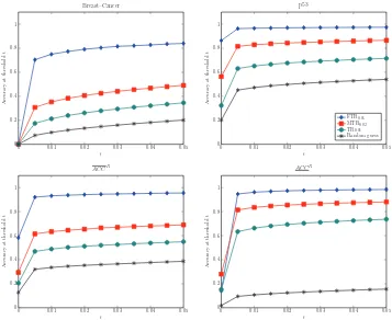
Overall Performance: The accuracies at t =0.05, Acci(t), Acc(t), and Acc(t) for the three

rules as well as the one achieved by guessing at random are shown in Figure 7. The Bonferroni

adjusted thresholds for MTR and TR were used: αFT R=0.05,αMT R=0.02,αT R=0.01 . Similar

figures for all sets of thresholds are shown in Appendix A, Section A.3. Over all predictions, the Full-Testing Rule achieves accuracy 96%, consistently higher than guessing at random, the MTR and the TR. The same results are also depicted in tabular form in Table 3, where additionally, the statistical significance is noted. The null hypothesis is that AccFT R_i (0.05)≤AccR_i(0.05), for R being MTR or TR. The one-tail Fisher’s exact test (Fisher, 1922) is employed when computationally

feasible, otherwise the Pearsonχ2test (Pearson, 1900) is used instead. FTR is typically performing

Covtype Read Infant-Mortality Compactiv Gisette Hiva Breast Cancer Lymphoma Wine Insurance C Insurance N 0

0.2

0.4

0.6

0.8

1

Ac

cu

ra

cy

a

t

t=

0

.0

5

p53 Ovarian C&C ACPJ Bibtex Delicious Dexter Nova Ohsumed Acc Acc

0

0.2

0.4

0.6

0.8

1

Ac

cu

ra

cy

a

t

t=

0

.0

5

F T R₀.05 M T R0.02 T R0.01 Random Guess

Figure 7: Accuracies Acci for each data set, as well as the average accuracy Acc (each data set

weighs the same) and the pooled accuracy Acc (each prediction weighs the same). All

accuracies are computed as threshold t=0.05. FTR’s accuracy is always above 80% and

always higher than MTR, TR, and random guess.

Sensitivity to the α parameter: The results are not particularly sensitive to the significance

thresholds used for α for MTR and TR. Figures 9 (a-b) show the average accuracy Acc and the

pooled accuracy Acc as a function of the al pha parameter used: no correction, Bonferroni correc-tion, and stricter than Bonferroni by one and two orders of magnitude. The accuracy of MTR and TR improves as they become more conservative but never reaches the one by FTR even for the

stricter thresholds ofαMT R=0.0002 andαT R=0.0001.

Sensitivity to t: The results are also not sensitive to the particular significance level t used to

define accuracy. Figure 8 graphs AccR_i(t) over t = [0,0.05]for two typical data sets as well as

Acc(t) and Acc(t). The situation is similar and consistent across all data sets considered, which

are shown in Appendix A. The lines of the Full Testing Rule rise sharply, which indicates that the p-values of its predictions are concentrated close to zero.

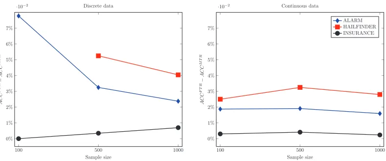
Explaining the difference of FTR and MTR: Asymptotically and when the data distribution is faithful to a MAG, the FTR and the MTR rules are both sound (100% accurate). However, when the distribution is not faithful, the performance difference could become large because FTR tests for faithfulness violations as much as possible in an effort to avoid false predictions. This may explain the large differences in accuracies observed in the Infant Mortality, Gisette, Hiva, Breast-Cancer, and Lymphoma data sets. When the distribution is faithful, but the sample is finite, we

expect some but small differences. For example when MTR falsely determines that X6⊥⊥Y|/0due to

a false positive test, the FTR rule still has a chance to avoid an incorrect prediction by additionally

testing X6⊥⊥Y|W . To support this theoretical analysis we perform experiments with simulated data

where the network structure is known. Specifically, we employ the structure of the ALARM (Bein-lich et al., 1989), INSURANCE (Binder et al., 1997) and HAILFINDER (Abramson et al., 1996)

Bayesian Networks. We sample 20 continuous and 20 discrete pairs of data sets D1 and D2 from

Data Set FTR0.05 MTR0.02 TR0.01 Random Guess

Covtype 1.00 1.00 0.91∗∗ 0.83∗∗

Read - 1.00 0.97 0.82

Infant Mortality 0.95 0.64∗∗ 0.36∗∗ 0.11♠

Compactiv 1.00 0.98 0.96∗ 0.93∗∗

Gisette 0.95 0.71♠ 0.59♠ 0.14♠

hiva 0.94 0.61♠ 0.44♠ 0.30♠

Breast-Cancer 0.84 0.49♠ 0.34♠ 0.20♠

Lymphoma 0.82 0.57♠ 0.39♠ 0.23♠

Wine 1.00 0.85 0.81 0.80

Insurance-C 0.97 0.75♠ 0.66♠ 0.37♠

Insurance-N 0.97 0.94∗ 0.86∗∗ 0.34♠

p53 0.97 0.87♠ 0.71♠ 0.54♠

Ovarian 0.99 0.98♠ 0.95♠ 0.91♠

C&C 0.96 0.88♠ 0.80♠ 0.77♠

ACPJ - 0.26 0.07 0.02

Bibtex 1.00 0.68 0.31 0.12∗∗

Delicious 1.00 0.87♠ 0.68♠ 0.23♠

Dexter - 0.50 0.05 0.02

Nova - 0.08 0.06 0.03

Ohsumed - 0.14 0.05 0.02

ACCR _{0.96 0.69}∗∗ _0.55∗∗ _0.39∗∗

ACCR _{0.98 0.88}♠ _0.74♠ _0.16♠

Table 3: ACCR_i (t)at t=0.05 with “Bonferroni” correction for rules FTR, MTR, TR and Random

Guess. Marks *, **, and♠denote a statistically significant difference from FTR at the

levels of 0.05, 0.01, and machine-epsilon respectively.

sample sizes 100, 500, 1000. Subsequently, we apply the FTR and MTR rules withαFT R=0.05

andαMT R=0.02 (Bonferroni adjusted) on each pair of D1 and D2 and all possible quadruples of

variables. The true accuracy is not computed on a test data set Dt but on the known graph instead

by checking whether Y and Z are d-connected given X and W . The mean true accuracies over all samplings are reported in Figure 10. The difference in performance on the faithful, simulated data is usually below 5%. In contrast, the largest difference in performance on the real data sets is over 35% (Breast-Cancer), while the difference of the pooled accuracies is 10%. Thus, violations of faithfulness seem to be the most probable explanation for the large difference in accuracy on the real data.

6.4 Summary, Interpretation, and Conclusions

We now comment and interpret the results of this section:

• Notice that even if all predicted pairs are truly correlated, the accuracy may not reach 100%

0 0.01 0.02 0.03 0.04 0.05 0

0.2 0.4 0.6 0.8 1 t Ac cu rac y at th re sh ol d t Breast–Cancer

0 0.01 0.02 0.03 0.04 0.05

0 0.2 0.4 0.6 0.8 1 t Ac cu rac y at th re sh ol d t p53

FTR0.05

MTR0

.02 TR0

.01 Random guess

0 0.01 0.02 0.03 0.04 0.05

0 0.2 0.4 0.6 0.8 1 t Ac cu rac y at th re sh ol d t ACCR

0 0.01 0.02 0.03 0.04 0.05 0

0.2 0.4 0.6 0.8 1 t Ac cu rac y at th re sh ol d t ACCR

Figure 8: Accuracies AccR_i(t) as a function of threshold t for two typical data sets along with

ACCR(t) and ACCR(t). The remaining data sets are plot in Appendix A Section A.3.

Predicted dependencies have p-values concentrated close to zero. The performance dif-ferences are insensitive to the threshold t in the performance definition.

• The FTR rule performs the test for the X-W association independently in both data sets.

Given that the data in our experiments come from exactly the same distribution, they could be pooled together to perform a single test; alternatively, if this is not appropriate, the p-values of the tests could be combined to produce a single p-value (Tillman, 2009; Tsamardinos and Borboudakis, 2010).

• The results show that the Full-Testing Rule accurately predicts the presence of dependencies,

statistically significantly better than random predictions, across all data sets, regardless of the type of data or the idiosyncracies of a domain. The rule is successful in gene-expression data, mass-spectra data measuring proteins, clinical data, images and others. The accuracy of predictions is robustly always above 0.80 and over all predictions it is 0.96; the difference with random predictions is of course more striking in data sets where the percentage of correlations (prior probability) is relatively small, as there is more room for improvement.

• The Full-Testing Rule is noticeably more accurate than the Minimal-Testing Rule, due to

in-duce models, but do not check whether the inin-duced model is Faithful. These results indicate that when the latter is not the case, the model (and its predictions) may not be reliable. On the other hand, the FTR rule is also noticeably more conservative: the number of predictions it makes is significantly lower than the one made by MTR. In some data sets (e.g., Compactiv, Insurance-N, and Ovarian) by using the MTR vs. the FTR one sacrifices a small percentage of accuracy (less than 3% in these cases) to gain one order of magnitude more predictions. However, caution should be exercised because in certain data sets MTR is over 35% less accurate than FTR.

• The Full-Testing Rule is more accurate than the Transitivity Rule. Thus, the performance

of the Full-Testing Rule cannot be attributed to simply performing a super-set of the tests performed by the Transitivity Rule.

• Predictions are the norm case and not occur in contrived or rare cases only. Even though

there were few or no predictions for a couple of data sets, there are typically hundreds or thousands of predictions for each data set. This is the case despite the fact that we are only looking for a special-case structure and the search for these structures is limited within groups of 50 variables for the larger data sets. The results are consistent with the ones in Triantafillou et al. (2010), where larger structures were induced from simulated data.

• FTR makes almost no predictions in the text data:3 this actually makes sense and is probably

evidence for the validity of the method: it is semantically hard to interpret the presence of a

word “causing” another word to be present.4

• FTR is an opportunistic algorithm that sacrifices completeness to increase accuracy, as well

as improve computational efficiency and scalability. General algorithms for co-analyzing data over overlapping variable sets, such as ION (Tillman et al., 2008), IOD (Tillman and Spirtes, 2011) and cSAT (Triantafillou et al., 2010) could presumably make more predictions, and more general types of predictions (e.g., also predict independencies). However, their computational and learning performance on a wide range of domains and high-dimensional data sets is still an open question and an interesting future direction to pursue.

7. Predicting the Presence of Conditional Dependencies

The FTR and the MTR not only predict the presence of the dependency Y6⊥⊥Z|/0given two data sets

on O1={X,Y,W}and O2={X,Z,W}; the rules also predict that either X◦ − ◦Y◦ − ◦Z◦ − ◦W or

X◦ − ◦Z◦ − ◦Y◦ − ◦W is the model that generated both data sets (see Algorithms 1 and 2). Both of these models also imply the following dependencies:

Y 6⊥⊥Z|X,

3. The only predictions in text data are in Bibtex (1 prediction) and in Delicious (856), which are the only text data sets that are actually not purely bag-of-words data sets but include variables corresponding to tags. 66% of the predictions made in Delicious involves tag variables, as well as the single prediction in Bibtex.

No Correction0 Bonferroni Bonferroni 10−1 Bonferroni 10−2 0.1

0.2

0.3

0.4

0.5

0.6

0.7

0.8

0.9

1

Ac

cu

rac

y

at

t

=

0.

05

FTR MTR TR Random Guess

No Correction0 Bonferroni Bonferroni 10−1 Bonferroni 10−2 0.1

0.2

0.3

0.4

0.5

0.6

0.7

0.8

0.9

1

Ac

cu

rac

y

at

t

=

0.

05

Figure 9: Average accuracy Acc(0.05)(left) and pooled accuracy Acc(0.05) (right) for each rule

as a function of α thresholds used: αMT R ∈ {0.05,0.02,0.002,0.0002} and αT R ∈ {0.05,0.01,0.001,0.0001} corresponding to no correction, Bonferroni correction, and stricter than Bonferroni by one and two orders of magnitude respectively. FTR’s perfor-mance is higher even when MTR and TR become quite conservative.

Y 6⊥⊥Z|W,

Y 6⊥⊥Z|{X,W}.

In other words, the rules predict that the dependency between Y and Z is not mediated by either X or W inclusively. To test whether all these predictions hold simultaneously at threshold t we compute:

p∗= max

S⊆{X,W}pY⊥⊥Z|S

and test whether p∗ ≤t. The above dependencies are all the dependencies that are implied by

the model but not tested by the FTR given that it has no access to the joint distribution of Y and

Z. Note that we forgo providing a value for p∗ when any of the conditional dependencies can

not be calculated, that is, when there are not enough samples to achieve large enough power, see Tsamardinos and Borboudakis (2010). The accuracy of the predictions for all dependencies in the model, named Structural Accuracy because it scores all the dependencies implied by the structure

of model, is defined in a similar fashion to Acc (Definition 11) but based on p∗instead of p:

SAccR_i(t) =#{p∗<=t,p∈M_iR}/|M_iR|.

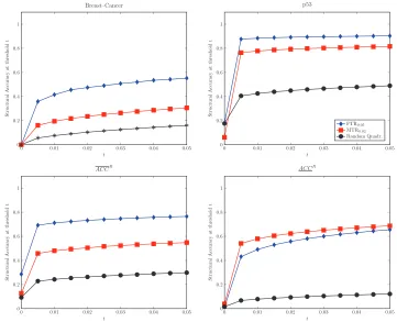
The SAcc for each FTR, MTR (with “Bonferroni” correction) and randomly selected quadruples is shown in Figure 7.1; the remaining data sets are shown in Appendix A. There is no line for the TR as it concerns triplets of variables and makes no predictions about conditional dependencies. Both

FTR and MTR have maximum p-values p∗ concentrated around zero. The curves do not rise as

sharp as those in Figure 8 since the p∗values are always larger than the corresponding pY⊥⊥Z|/0. We

also calculate the accuracy at t =0.05 for all data sets (see Table 9 in Appendix A Section A.2).

The results closely resemble the ones reported in Table 3, with FTR always outperforming random

guess. FTR outperforms MTR on most data sets (and hence SACCFT R>SACCMT R; however, over

100 500 1000 0%

1% 2% 3% 4% 5% 6% 7%

·10−2

Sample size

AC

C

F

T

R

−

AC

C

M

T

R

Discrete data

100 500 1000

0% 1% 2% 3% 4% 5% 6% 7%

·10−2

Sample size

AC

C

F

T

R

−

AC

C

M

T

R

Continuous data

ALARM HAILFINDER INSURANCE

Figure 10: Difference between ACCFT Rand ACCMT Rfor discrete (left) and continuous (right)

sim-ulated data sets. Results calcsim-ulated using the “Bonferroni” correction (i.e., FTR0.05and

MTR0.02). The difference between FTR and MTR is larger than 5% only in two cases

with low sample size (ALARM and HAILFINDER networks); however, the difference steeply decreases as the sample size increases. No prediction was made for HAIL-FINDER with discrete data and 100 samples. The difference between FTR and MTR on faithful data is relatively small.

7.1 Summary, Interpretation, and Conclusions

The results show that both the FTR and MTR rules correctly predict all the dependencies (con-ditional and uncon(con-ditional) implied by the models involving the two variables never measured to-gether. These results provide evidence that these rules often correctly identify the data generating structure.

8. Predicting the Strength of Dependencies

In this section, we present and evaluate ideas that turn the qualitative predictions of FTR to quanti-tative predictions. Specifically, for Example 1 we show how to predict the strength of dependence in addition to its existence. In addition to the Faithfulness Condition, we assume that when the

FTR applies on quadruple{X,Y,Z,W}, all dependencies are linear with independent and normally

distributed error terms. However, the results of these section could possibly be generalized to more relaxed settings, for example, when some of the error terms are non-Gaussian (Shimizu et al., 2006, 2011). When the Full-Testing Rule applies, we can safely assume the true structure is one of the MAGs shown in Figure 5. Given linear relationships among the variables, we can treat these MAGs as linear Path Diagrams (Richardson and Spirtes, 2002). We also consider normalized versions of the variables with zero mean and standard deviation of one. Let us consider one of the possible MAGs:

M1: X

ρXY