Eighteenth Order Convergent Method for Solving Non-Linear Equations

COMPUTER SCIENCE & TECHNOLOGY

www.computerscijournal.org

March 2017, Vol. 10, No. (1): Pgs. 144-150 An International Open Free Access, Peer Reviewed Research Journal

Published By: Oriental Scientific Publishing Co., India.

Eighteenth Order Convergent Method

for Solving Non-Linear Equations

V.B. KUMAR VATTI

1

_{, RAMAdEVI SRI}

1

_{and M.S.KUMAR MYLAPALLI}

2

1_{Dept. of Engineering Mathematics, Andhra University, Visakhapatnam, India.} 2_{Dept. of Engineering Mathematics, Gitam University, Visakhapatnam, India.}

*Corresponding author E-mail: [email protected]

http://dx.doi.org/10.13005/ojcst/10.01.19

(Received: March 03, 2017; Accepted: May 17, 2017)

ABSTRACT:

In this paper, we suggest and discuss an iterative method for solving nonlinear equations of the type f(x) = 0 having eighteenth order convergence. This new technique based on Newton’s method and extrapolated Newton’s method. This method is compared with the existing ones through some numerical examples to exhibit its superiority.

AMS Subject Classification: 41A25, 65K05, 65H05.

Keywords: Iterative method, Nonlinear equation, Newton’s method,

Convergence analysis, Higher order convergence.

INTROdUCTION

We consider finding the zero’s of a nonlinear equation

f(x)=0 ...(1.1)

Where f D R: ⊂ →Ris a scalar function on an open interval D and f(x) may be algebraic, transcendental or combined of both. The most widely used algorithm for solving (1.1) by the use of value of the function and its derivative is the well known quadratic convergent Newton’s method (NM) given by

( )

( )

1

f xn

x

_n

_xn

f xn

=

−

+

_′

...(1.2)

(n=0,1,2,...)

starting with an initial guess x₀ which is in the vicinity of the exact root x*. The efficiency index of Newton’s method is

2 2 1.4142

₌

.

The Extrapolated Newton’s method (ENM) suggested by V.B.Kumar, Vatti et.al 11 _{which is} developed by extrapolating Newton’s method (1.2) introducing a parameter ‘an’ given by

(

1

)

( )

_{( )}

1

f xn

x

_n

_{n n}

x

_{n n}

x

f xn

a

a





= −

+

_

−

_

+

_

_′

_





( )

( )

1

f xn

x

_n

_xn

_n

f xn

a

⇒

₊

=

−

′

...(1.3)

Here, the optimal choice for the parameter ‘an’ is

2

2

n

n

a

ρ

=

−

...

(1.4)

Where

( ) ( )

( )

2

f x f x

_n

_n

n

f xn

ρ

=

′′

′









_...

...

(1.5)

Combining (1.3), (1.4) and (1.5), one can have

( )

( )

_{( ) ( )}

( )

1 1

1 ₂

2 f xn

x_{n xn}

f xn _{f x f xn n}

f xn

= − ⋅

+ _{′  }

′′

 ₋ 

 _{ ′ } 

   

 

...(1.6)

(n=0,1,2,...)

Which is same as Halley’s method having third order convergence requires three functional evaluations. The efficiency index of this method is

3 3 1.4422

=

.

A three step Predictor-corrector Newton’s Halley method (PCNH) suggested by Mohammed and Hafiz 10 _{(see[1 to 10]), is given by:}

For a given x₀, we compute x_n+1by using

( )

( )

( ) ( )

( )

( ) ( )

( )

( )

( )

_{( )}

( )

(

)

2

2

3 2

2

1 ₂

0,1,2,...

f xn w_n x_{n f xn}

f w f w_{n n} y_n w_n

f w_n f w f w_{n n}

f y f y

f y_{n n n}

x_{n yn}

f y_{n f yn}

n



= − _

′ _



′ _

= −



′ ′′

  −

  

 ′′

  _

 

= − − _

+ ′ _{ ′ }

  



= _

...(1.7)

This method has eighteenth order convergence and its efficiency index is

818 1.4352

=

In section 2, we develop and discuss a three step iterative method and the convergence criteria is discussed in section 3. Few numerical examples are considered to show the superiority of this method in the concluding section.

Eighteenth Order Convergent Method (Eocm)

Consider x* be the exact root of (1.1) in an open interval D in which f(x) is continuous and has well defined first and second derivatives. Let x_n be the nth _{approximate to the exact root x* of (1.1)}

and

x

∗ = +

x

_n

e

_n

...(2.1)

where is the error at the nth _stage.

Therefore, we have

( )

0

f x

∗ =

...(2.2)

Expanding by Taylor’s series about, we have

( )

( )

(

)

( )

(

)

2

_{( )}

_{. . .}

2!

f x

f x

_n

x

x f x

_n

_n

x

_xn

f xn

∗

₌

₊

∗

₋

_′

∗ −

′′

+

+

...(2.3)

( )

( )

( )

2

( )

. . .

2

en

f x

∗

=

f x

_n

+

e f x

_n

′

_n

+

f x

′′

_n

+

...(2.4)

Assuming

en

is small enough and neglecting higher powers of

en

starting from

en

3

onwards, we obtain from (2.2) and (2.4) as

( )

( )

( )

2

₂

₂

₀

e f x

_n

′′

_n

+

e f x

_n

′

_n

+

f x

_n

=

( )

( )

( ) ( )

( )

2 4 8 2

e_n  f x′ _n f x′ _n f x f x_n ′′ _n  f x′′ _n

⇒ = −_ ± − _

Where

( ) ( )

( )

ˆ

f x f x

n

₂

n

f xn

ρ

=

′′

′









...(2.5)

Now,

( )

( )

ˆ

ˆ

1

1 2

1

1 2

ˆ

1

1 2

f xn

en

= −

_{f xn}

′





−

−

ρ

 

 

+

_ρ

−

ρ





′′



_

+

−



_

i.e.,

( )

( )

2 1

ˆ

1 1 2

f xn

en= − _{f xn} _{ ρ}_ ′  + − 

...(2.6)

( )

( )

_{( ) ( )}

( )

2 1

1

1 1 2 ₂

f xn

x_{n xn}

f xn _{f x f xn n}

f xn

= − ⋅

+ _{′  }

′′

 _{+ −} 

 

′

 

   

 

...(2.7)

This scheme (2.7) allows us to propose the following algorithm with the method (1.2) as the first step and the method (1.6) as the second step.

Algorithm 2.1: For a given

x

₀

, compute

xn

₊

₁

by the iterative schemes

( )

( )

f xn

w

_n

x

n f xn

=

−

′

...(2.8)

( )

( )

1

1

ˆ

2

f wn

y

_n

w

_{n f wn}

ρ





=

−

_

_

′

_

−

_

...(2.9)

Where

( ) ( )

( )

ˆ

_n

f w f w

n

₂

n

f wn

ρ

=

′′

′









...(2.10)

( )

( )

2

1

1

f yn

₁

_{1 2}

x

_n

_yn

f yn

ρ

n





=

−





+

_′

_

₊

₋

_





...(2.11)

(n=0,1,2,...)

Where

( ) ( )

( )

2

f y f y

_n

_n

n

f yn

ρ

=

′′

′









...(2.12)

This algorithm (2.1) requires 3 functional evaluations, 3 of its first derivatives and 2 of its second derivatives and can be called as Eighteenth order Convergent Method (EOCM).

Convergence Criteria

Theorem 3.1. Let x*∈D be a single zero of a sufficiently differentiable function

f D R

:

⊂ →

R

for an open interval D. If x₀ is in the vicinity of x*, then the algorithm (2.1) has eighteenth order convergence.

Proof: Let x* be a single zero of (1.1) and

*

x

=

x

_n

+

e

_n

...(3.1)

Then,

f x

( )

∗ =

0

...(3.2)

If xn be the nth approximate to the root of (1.1), then expanding

f xn

( )

about x* using Taylor’s expansion, we have

( )

( ) ( )

( )

( )

( )

*

*

2

_*

3

* . . .

2!

3!

f x

_n

f x

e f x

_n

e

_n

_{f x}

e

_n

_f

_x

f xn

′

=

+

′′

′′′

+

+

+

( )

( )

( )

( )

( )

( )

( )

( )

* *

1 ₂ 1 ₃

* *

2! 3!

*

*

1 _{4 . . .} *

4!

f x f x

e_n e_n e_n

f x f x

f x _{f xn}

v

f x

en f x

 _{′′ ′′′} 

 _{+ +} 

 _{′ ′} 

 

′

=  

 ′ 

_{+ +} 

 _′ 

 

 

( )

*

2

3

_{4 ...}

2

3

4

f x

′



e

_n

c e

_n

c e

_n

c e

_n



=

_

_

+

+

+

+

_

_

...(3.3) Where

( )

( )

(

)

1

_,

_{2, 3, 4, . . .}

!

j

j

f x

c

j

j

f x

∗

∗

=

⋅

=

′

And,

( )

( )

* 1 2 ₂ 3₃ 2 4 ₄ 3 . . .

f x′ _n = f x′ _ + c e_n+ c e_n + c e_n + _

...

(3.4) Now,

( )

( )

(

)

(

)

( )

2

₂

₂

2

3

2

3

2

3

4

5

3

₄

7

_{2 3}

4

₂

f xn

_e

_{c e}

_c

_c

_e

n

n

n

f xn

c

c c

c

e

_n

o e

_n

=

−

−

−

′

−

−

+

+

...(3.5)

From (2.8), (3.1) and (3.5), we have

(

)

(

)

( )

2

₂

₂

2

3

2

3

2

3

4

5

3

₄

7

_{2 3}

4

₂

w

_n

x

c e

_n

c

c

e

_n

c

c c

c

e

_n

o e

_n

∗

=

+

+

−

+

−

+

+

...(3.6)

Then, expanding_{f w}

( ) ( ) ( )

_{n , f w}′ _{n , f w}′′ _n

about X* by using (3.6), we obtain

( )

( )

(

)

( )

(

)

_{( )}

(

)

_{( )}

* * 2 3 * _{* . . .} 2! 3!

f w_n f x w_n x f x

w_n x w_n x

f x f x

∗ _′ = + − ∗ ∗ − − ′′ ′′′ + + + ...(3.8)

( )

*

2

3

_{4 ...}

2

3

4

f x W c W

′



c W

c W



=

_

_

+

+

+

+

_

_

_...(3.9)

( )

( )

(

)

( )

(

)

_{( )}

*

*

2

* . . .

2!

f w

_n

f x

w

_n

x f x

w

_n

x

f

x

∗

′

=

′

+

−

′′

∗

−

′′′

+

+

...(3.10)

Combining (3.6) to (3.10) as done in [10] and from (2.9), we obtain

y

_n

=

x

∗

+

T

...(3.11)

where _T=

(

_c22−_{c W3}

)

3 ...(3.12)

Now, expanding f y

( ) ( )

_n , f y′ _n , f y′′

( )

_n

about X* by using (3.11), we obtain

( )

( )

* ₂ 2 ₃ 3 ₄ 4 ...

f y_n = f x′ _T c T+ +c T +c T + _ ...(3.13)

( )

( )

* _{1 2 3} 2 ₄ 3 ₅ 4 _... 5

2 3 4

f y′ _n =f x′ _ + c T+ c T + c T + c T + _  

...(3.14)

( )

( )

* 2 2 6 3 12 4 2

3 4

20₅ 30 ₆ ...

c c T c T

f y_n f x

c T c T

 _{+ +}    ′′ = ′ _{ } + + +     ...(3.15)

and

( ) ( )

( )

2

f y f y

_n

_n

n

f yn

ρ

=

′′

′









(

)

(

)

(

)

(

) (

) (

)

(

)

...

48 27 1 ...

2 2 3 2 4 2₂ 6₃ 2₂ 12₄ 8_{2 3} 20₅ 14_{2 4} 6₃

2 2 3 3 3 3 12 6 36 32 8 36 32 8 2 2 3 2 3 2 4 2 3 2 4

4 2 2 4 80₂ 144_{2 3 2 4 3 0 5}

1 4

T T T T

T T T T

T

c c c c c c c c c c c c c c c c c c c c c c c c c c c c

+ + + + + + − + − + + + − + + + + + = − − − − −

2 3 _{4 ...}

1 2 3 4

PT P T P T P T

= + + + + _...(3.18)

where,

P

₁

=

2

c

₂

, P₂= −6c₂2+6c₃,

,

3

16

28

12

3

2

2 3

4

P

=

c

−

c c

+

c

2

4

2

100

40

50

30

_{20 5}

4

2 3

2

2 4

3

P

=

c c

−

c

−

c c

−

c

+

c

Now,

2 3

2

1 1

1 2 _{1 1 2 3 1 2}

2 2

2

3 5

3 2 2 4 4 _...

4 ₂ 1 3 ₂ 1 2 ₈ 1

P P

PT P T P P P T

n

P

P P P P P P T

ρ    

− = − + − − + − − −             + −_ − − − − _ +

  _...(3.17)

and,

2 3

2 3 3

1 1 2 1 2 1 1

2 4 2 2 2 4 1 1 2 2

2 _{3 5}

2 4 4 1 3

4 2 _...

1 2 1 2 4 2 4 16

P

P P P P P P

T T T

n

P P

P P

P P P T

ρ        _{− −} ₊  ₋ _{+ +}               + − _{=  }   _{− + + + +  +}   _{ }   _{ }   

2 3 4

1+ 1 2− ρ_n=2 1__ +M T M T₁ + ₂ +M T₃ +M T₄ +...__

...(3.18) where,

M

₁

= −

c

₂

,

M

₂

=

2

c

₂

2

−3 ,

c

₃

3

4

8

6 ,

3

2

2 3

4

M

=−

c

+

c c

−

c

2

4

4

4

13

4

2 3

2

2 4

M

=−

c c

+

c

+

c c

−

_{3 3}

c

2

10 5

c

−

Now again,

(

) (

)

(

)

2 2 3 3

1 2

1 1 1 1 2 1 2 3 1 1 1 2

2 2 4 4

2 _{2 3 ...}

2 1 4 4 1 2 1

M T M M T M M M M T n

M M M M M M M T

ρ _{− + − + − −}  −   + −  _{=  }   _{+ + − − + +}    

1 1 2 3 4

1 1 2 1 _{1 2 3 4} . . .

2 N T N T N T N T

n

ρ −  

 + −  = _ + + + + + _

   

...(3.19)

Where, _,

1

2

N

=

c

N

₂

= −

c

₂

2

+3 ,

c

₃

3 2

6 ,

3

2

2 3

4

N

=

c

−

c c

+

c

2

4

2

15

3

12

_{10 5}

4

2 3

2

2 4

3

N

= −

c c

+

c

−

c c

+

c

+

c

From (3.13) and (3.14), we obtain

( )

( )

(

)

(

)

( )

2 ₂ 2 ₂ 3

2 2 3

3 4 5

7 _{2 3} 4 ₂ 3 ₄

f yn _{T c T c c T}

f yn

c c c c T_n o T

= − + − +

′

− − +

Considering the first degree and second degree terms of the expression lying within the square brackets of the formula (3.23) and from the algorithm 2.1, we have the following two more algorithms.

Algorithm 3.1: For a given, compute by the iterative

schemes

( )

( )

f xn w_n=x_{n f xn}−

′

( )

( )

1

1

n

2

f wn

y

_n

w

_{n f wn}

ρ





=

−

_

_

′

_

−

_

Where

( ) ( )

( )

2

f w f w

_n

_n

n

f wn

ρ

=

′′

′









( )

( )

( )

_{( )}

( )

2 3

1

f y

n

f y

₂

n

f y

n

x

_n

_yn

f y

_n

_{f y}

_n

′′









=

−

−

+

_′

_

_′

_





(n=0,1,2,...)

which is same as the eighteenth order convergent method proposed by Mohammed and Hafiz 10_.

Algorithm 3.2: For a given

x

₀, compute

xn

₊

₁

by the iterative schemes

( )

( )

f xn

w

_n

=

x

_{n f xn}

−

′

( )

( )

1 1n 2 f wn

y_n w_{n f wn}

ρ

 

= − _{ }

′ _ − _

Where

( ) ( )

( )

ˆ_n f w f wn ₂n

f wn

ρ = ′′ ′

 

 

( )

( )

( )

_{( )}

( )

( )

_{( )}

( )

2 3 2

3 5

1 f yn f y₂n f yn f y₂n f yn

x_{n yn}

f y_{n f yn f yn}

′′ ′′

     

     

= − − −

+ _{′  ′   ′ }

   

As done in convergence criteria above in section 3, one can easily obtain.Therefore, the algorithm (3.2) has eighteenth order convergence.

From (3.19) and (3.20), we obtain

( )

( )

(

)

_{( )}

1 ₂

ˆ

1 1 2 _{1 2}

2 3

2 2

2 1 2 2 3

2

2 2

3 2 2 1 2 3 4 5

3 7_{2 3} 4₂ 3₄

f yn _{n T N c T}

f yn

N N c c c T

N N c N c c

T_n o T c c c c

ρ −  

 

⋅ +_ − _ = +_ − _

′

 

+_ − + − _

 _{− + − +}

 

+_{ } +

− −

 

 

[ ]₀ 2 3 3 2 2 1

(

222 23

)

4

( )

5

3 ₃

7_{2 3} 4₂ 3₄

N N c N c c

T T c T T_n o T

c c c c

 _{− + −} 

 

 

= + +_{ } +_{ } +

+ − −

 

 

...(3.21)

Combining (3.13) to (3.21) and from (2.11), we obtain

* _{3 ...}

1 3

x_n+ =x + −T _T c T+ + _

*

_{3 ...}

3

x

c T

=

−

+

(

)

3

* 2 3 _{. . .}

3 2 3

x c  c c W 

= − _ − _ +

 

i.e., e_{n+1 3 2}=c c

(

2−c₃

)

3W9 ...+

(

₂

)

3 ₂

(

₂

)

₃ 9

2 2 . . .

1 3 2 3 2 3 2

e_n c c c c e_n c c e_n 

⇒ ₊ = − _ + − _ +

 

(

)

3

( )

9 2 18 19

1 3 2 2 3

e_n c c c c e_n o e_n

⇒ ₊ = − +

...(3.22)

Hence, this method has eighteenth order convergence and its efficiency index is

818 1.4352

=

.

Case 3.1: By expanding _{1 2}− _ρn appearing in the denominator of the third step of algorithm 2.1, we obtain

( )

( )

2 3

2 1

1

2

2 2

f yn x_{n yn}

f yn _ρn ρn ρn

= − ⋅

+ _{′  }

− − −

 

 

( )

( )

2 ₅ 3

1

1 f yn ₂n ₂n ₈n

x_{n yn}

f yn

ρ ρ ρ

 

⇒ ₊ = − _ + + + _

′ _{ }

...(3.23)

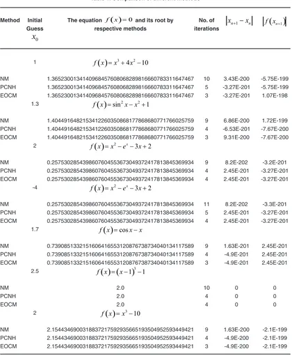
Table 1: Comparison of different methods

Method Initial The equation f x

( )

=0 and its root by No. of

x

_n+1

−

x

_{n f x}

( )

_n+1

Guess respective methods iterations

0

x

1 _{f x}

( )

_=x3_+4x2₋₁₀

NM 1.3652300134140968457608068289816660783311647467 10 3.43E-200 -5.75E-199 PCNH 1.3652300134140968457608068289816660783311647467 5 -3.27E-201 -5.75E-199 EOCM 1.3652300134140968457608068289816660783311647467 3 -3.27E-201 1.07E-198

1.3 _{f x}

( )

_=sin2_{x x−} 2₊₁

NM 1.4044916482153412260350868177868680771766025759 9 6.86E-200 1.72E-199 PCNH 1.4044916482153412260350868177868680771766025759 4 -6.53E-201 -7.67E-200 EOCM 1.4044916482153412260350868177868680771766025759 3 9.31E-200 -7.67E-200

2 _{f x}

( )

_=x2_−ex_−3x+2

NM 0.2575302854398607604553673049372417813845369934 9 8.2E-202 -3.2E-201 PCNH 0.2575302854398607604553673049372417813845369934 4 2.45E-201 -3.27E-201 EOCM 0.2575302854398607604553673049372417813845369934 4 2.45E-201 -3.27E-201

-4 _{f x}

( )

_=x2_−ex_−3x+2

NM 0.2575302854398607604553673049372417813845369934 11 8.2E-202 -3.3E-201 PCNH 0.2575302854398607604553673049372417813845369934 5 2.45E-201 -3.27E-201 EOCM 0.2575302854398607604553673049372417813845369934 4 2.45E-201 -3.27E-201

1.7 _{f x}

( )

=_{cosx x}−

NM 0.7390851332151606416553120876738734040134117589 9 1.63E-201 2.45E-201 PCNH 0.7390851332151606416553120876738734040134117589 4 -4.9E-201 2.45E-201 EOCM 0.7390851332151606416553120876738734040134117589 3 -4.9E-201 2.45E-201

2.5 _{f x}

( ) (

_{= x−1}

)

3₋₁

NM 2.0 10 0 0

PCNH 2.0 4 0 0

EOCM 2.0 4 0 0

2 _{f x}

( )

_=x3₋₁₀

NM 2.1544346900318837217592935665193504952593449421 9 1.63E-200 -2.1E-199 PCNH 2.1544346900318837217592935665193504952593449421 4 -4.9E-200 -2.1E-199 EOCM 2.1544346900318837217592935665193504952593449421 3 -4.9E-200 -2.1E-199

Numerical Examples

We consider the same examples considered by Mohammed and Hafiz10 _and compared EOCM with NM and PCNH methods. The computations are carried out by using

mpmath-PYTHON software programming and comparison of number of iterations for these methods are

obtained such that 201

1

10

n n

x

x

−

+

−

<

and

( )

201

1

10

n

f x

−

The above computational results exhibit the superiority of the new method EOCM over the

Newton’s method and PCNH method in terms of number of iterations and accuracy.

REFERENCES

1. I.K. Argyros, S.K. Khattri, An improved semi local convergence analysis for the Chebyshev method, Journal of Applied

Mathematics and computing, 42(1, 2)

(2013), 509-528, doi: 10.1007/s12190-013-0647-3.

2. M.A. Hafiz, Solving nonlinear equations using steffensen-type methods with optimal order of convergence, Palestine Journal of

Mathematics, 3(1) , 113-119, (2014).

3. M.A. Hafiz, A new combined bracketing method for solving nonlinear equations,

Journal of Mathematical and Computational Science, 3,(1)(2013).

4. M.A. Hafiz, S.M.H. Al-Goria, Solving nonlinear equations using a new tenth-and seventh- order methods free from second derivative, International Journal

of Differential Equations and Applications, 12(3) (2013), 169-183,2013, doi: 10.12732/

ijdea.v12i3.1344.

5. S.K. Khattri, Torgrim Log, Constructing third-order derivative-free iterative methods, Int.

J. Comput. Math., 88(7), (2011), 1509-1518,

doi: 10.1080/00207160.2010520705. 6. S.K. Khattri, Quadrature based optimal

iterative methods with applications in high precision computing, Numer. Math. Theor.

Meth. Appl., 5, 592-601, (2012).

7. S.K. Khattri, Trond Steihaug, Algorithm for forming derivative-free optimal methods, ,

Numerical Algorithms, (2013), doi: 10.1007/

s11075-013-9715-x.

8. Mohamed S.M. Bahgat, M.A. Hafiz, New two-step predictor-corrector method with ninth order convergence for solving nonlinear equations, Journal of Advances

in Mathematics ,2, 432-437, (2013).

9. K h a l i d a I n aya t N o o r, M u h a m m a d Aslam Noor, Shaher Momani, Modified Householder iterative methods for nonlinear equations”, Applied Mathematics and

Computation,190, 1534-1539, (2007), doi:

10.1016/j.amc.2007.02.036.

10. Mohamed S.M. Bahgat, M.A. Hafiz, Three-step iterative method with eighteenth order convergence for solving nonlinear equations, Int. Journal of Pure and Applied

Mathematics, 93,(1), 85-94, 2014.

11. Vatti V.B.Kumar, Mylapalli M. S. Kumar, Katragadda A. Kumari,Extrapolated Newton- Raphson Method, Math. Educ. 43(1),