Multivariate Convex Regression with Adaptive Partitioning

Multivariate Convex Regression with Adaptive Partitioning

Lauren A. Hannah [email protected]

Department of Statistics Columbia University New York, NY 10027, USA

David B. Dunson [email protected]

Department of Statistical Science Duke University

Durham, NC 27708, USA

Editor: Hui Zou

Abstract

We propose a new, nonparametric method for multivariate regression subject to convexity or con-cavity constraints on the response function. Convexity constraints are common in economics, statistics, operations research, financial engineering and optimization, but there is currently no multivariate method that is stable and computationally feasible for more than a few thousand ob-servations. We introduce convex adaptive partitioning (CAP), which creates a globally convex regression model from locally linear estimates fit on adaptively selected covariate partitions. CAP is a computationally efficient, consistent method for convex regression. We demonstrate empir-ical performance by comparing the performance of CAP to other shape-constrained and uncon-strained regression methods for predicting weekly wages and value function approximation for pricing American basket options.

Keywords: adaptive partitioning, convex regression, nonparametric regression, shape constraint, treed linear model

1. Introduction

Consider the regression model for x_∈

X

y= f0(x) +ε,

where f0:Rp→Randεis a mean 0 random variable. In this paper, we study the situation where f0is convex. That is,

λf0(x1) + (1−λ)f0(x2)≥ f0(λx1+ (1−λ)x2),

for every x1,x2∈

X

estimate f0 subject to the convexity constraint. Convex regression is easily extended to concave regression since a concave function is the negative of a convex function.

problems in operations research and reinforcement learning can be solved with response surfaces (Lim, 2010) or value-to-go functions. These exhibit concavity in many settings, like resource al-location (Topaloglu and Powell, 2003; Powell, 2007; Toriello et al., 2010) or stochastic control (Keshavarz et al., 2011). Similarly, efficient frontier methods like data envelopment analysis (Kuos-manen and Johnson, 2010) include convexity constraints. In density estimation, shape restrictions like log-concavity provide flexible estimators without tunable parameters (Cule et al., 2010; Cule and Samworth, 2010; Schuhmacher and D¨umbgen, 2010). Finally, in optimization, convex approxi-mations to polynomial constraints are valuable for geometric programming (Kim et al., 2004; Boyd et al., 2007; Magnani and Boyd, 2009).

Although convex regression has been well explored in the univariate setting, the literature re-mains underdeveloped in the multivariate setting. Methods where an objective function is con-strained to the set of convex functions through supporting hyperplane constraints for each pair of observations (Hildreth, 1954; Holloway, 1979; Kuosmanen, 2008; Seijo and Sen, 2011; Lim and Glynn, 2012; Allon et al., 2007) or semidefinite constraints over all observations (Roy et al., 2007; Aguilera and Morin, 2008, 2009; Henderson and Parmeter, 2009; Wang and Ni, 2012) are too com-putationally demanding for more than a few thousand observations.

In more recent approaches, different methods have been developed. Fitting a convex hull to a smoothed version of the data (Aguilera et al., 2011) scales to larger data sets, but is inefficient for more than 4 or 5 dimensions. Refitting a series of hyperplanes can be done in a frequentist (Magnani and Boyd, 2009) or Bayesian (Hannah and Dunson, 2011) manner. While the Bayesian method does not scale to more than a few thousand observations, the frequentist method scales to much larger data sets but can exhibit unstable behavior. Recent literature is more fully reviewed in Section 2.

In this paper, we introduce the first computationally efficient and theoretically sound multivari-ate convex regression method: convex adaptive partitioning (CAP). It fits a series of hyperplanes to the data through adaptive partitioning. It relies on an alternate, first-order definition of convexity,

f0(x1)≥ f0(x2) +g0(x2)T(x1−x2), (1) for every x1,x2∈

X

The CAP estimator is formed by adaptively partitioning a set of observations in a method similar to trees with linear leaves (Chaudhuri et al., 1994). Within each subset of the partition, we fit a linear model to approximate the subgradient of f0within that subset. Given a partition with K subsets and linear models,(αk,βk)Kk=1, a continuous, convex (concave) function is then generated by taking the maximum (minimum) over the hyperplanes by

fn(x) = max

k_∈{1,...,K_}αk+β T kx.

The partition is refined by a twofold strategy. First, one of the subsets is split along a cardinal direction (say, x1or x3) to grow K. Then, the hyperplanes themselves are used to refit the subsets. A piecewise linear function like fn induces a partition; a subset is defined as the region where a

fit with complexity using a generalized cross validation method (Golub et al., 1979; Friedman, 1991). We show that CAP is consistent with respect to the ℓ∞ metric. Because of the dramatic reduction in runtime, CAP opens a new class of problems for study, namely moderate to large problems with convexity or concavity constraints.

2. Literature Review

The literature for convex regression is scattered throughout a variety of fields, including statistics, operations research, economics numerical analysis and electrical engineering. Most methods are de-signed for the univariate setting, which is closely related to isotonic regression. Univariate methods rely on the ordering implicit to the real line. Setting xi−1<xi<xi+1for i=2, . . . ,n−1,

f0(xi)₋f0(xi₋1) xi−xi−1 ≤

f0(xi+1)−f0(xi) xi+1−xi

, i=2, . . . ,n₋1, (2)

is equivalent to Equation (1). When f0is differentiable, Equation (2) is equivalent to an increasing derivative function.

The oldest and simplest solution method is the least squares estimator (LSE), which produces a piecewise linear estimator by solving a quadratic program with a least squares objective function subject to the constraints in Equation (2) (Hildreth, 1954; Dent, 1973). Although the LSE is com-pletely free of tunable parameters, the estimator is not smooth and can overfit in boundary regions. Consistency, rate of convergence, and asymptotic distribution were shown by Hanson and Pledger (1976), Mammen (1991) and Groeneboom et al. (2001), respectively. Algorithmic methods for solving the quadratic program were given in Wu (1982); Dykstra (1983) and Fraser and Massam (1989).

Splines use linear combinations of basis functions to produce a smooth estimator; in univari-ate convex regression, an increasing function can be fit to the derivative of the original function. Meyer (2008) and Meyer et al. (2011) used convex-restricted splines with positive parameters in frequentist and Bayesian settings, respectively. Turlach (2005) and Shively et al. (2011) used unre-stricted splines with reunre-stricted parameters in frequentist and Bayesian settings, respectively. In other methods, Birke and Dette (2007) used convexity constrained kernel regression. Chang et al. (2007) used a random Bernstein polynomial prior with constrained parameters. Due to the constraint on the derivative of f0, univariate convex regression is quite similar to univariate isotonic regression; see Brunk (1955), Hall and Huang (2001), Neelon and Dunson (2004) and Shively et al. (2009) for examples.

In the multivariate setting Equation (1) cannot be reduced to a set of n₋1 linear inequalities. Instead, it needs to hold for every pair of points. The multivariate least squares estimator Hildreth (1954); Holloway (1979) solves the quadratic program,

min

n

∑

(yi−yˆi)2 (3)

subject to ˆyj≥yˆi+gTi (xj−xi), i,j=1, . . . ,n.

Here, ˆyi and gi are the estimated values of f0(xi)and the subgradient of f0at xi, respectively. The

estimator f_nLSE is piecewise linear,

f_nLSE(x) = max

i∈{1,...,n}yˆi+g T

The characterization (Kuosmanen, 2008) and consistency (Seijo and Sen, 2011; Lim and Glynn, 2012) of the least squares problem have only recently been studied. The LSE quickly becomes impractical due to its size: Equation (3) has n(n₋1) constraints. This results in a computational complexity of

O

An alternative to first order constraints in Equation (1) is second order, or Hessian, constraints. Roy et al. (2007) and Aguilera and Morin (2008, 2009) solved a math program with a least squares objective function and semidefinite constraints through semidefinite programming. Henderson and Parmeter (2009) used kernel smoothing with a restricted Hessian and found a solution with sequen-tial quadratic programming. While these methods are consistent in some cases (Aguilera and Morin, 2008, 2009), they are computationally infeasible for more than about a thousand observations.

Recently, multivariate convex regression methods have been proposed with different approaches. Aguilera et al. (2011) proposed a two step smoothing and fitting process. First, the data were smoothed and functional estimates were generated over anε-net over the domain. Then the convex hull of the smoothed estimate was used as a convex estimator. Again, although this method is con-sistent, it is sensitive to the choice of smoothing parameter and does not scale to more than a few dimensions. Hannah and Dunson (2011) proposed a Bayesian model that placed a prior over the set of all piecewise linear models. They were able to show adaptive rates of convergence, but the in-ference algorithm did not scale to more than a few thousand observations. Koushanfar et al. (2010) transformed the ordering problem associated with shape constrained inference into a combinatorial optimization problem which was solved with dynamic programming; this scales to a few hundred observations.

The work that is closest to CAP is an iterative fitting scheme of Magnani and Boyd (2009). In this method, the data were divided into K random subsets and a linear model was fit within each subset; a convex function was generated by taking the maximum over these hyperplanes. This new function induced a partition over the covariate space, which generated a new collection of K subsets. Again, linear models were fitted and another convex function was produced by taking the maximum over the new hyperplanes. This sequence was repeated until convergence. Although this method usually produces a high quality estimate, it does not always converge and can be unstable.

3. Convex Adaptive Partitioning

A natural way to model a convex function f0is through the maximum of a set of K hyperplanes. We do this by partitioning the covariate space and approximating the gradients within each region by hyperplanes generated by the least squares estimator. The covariate space partition and K are chosen through adaptive partitioning. Given a partition_{A1, . . . ,AK}of

X

each subset can be created by taking the least squares linear estimate based on all of the observations within that region,

(αk,βk) =arg min

α,β _{i : x}

∑

yi−α−βTxi

A convex function ˆf can be created by taking the maximum over(αk,βk)Kk=1, ˆ

fn(x) = max

k∈{1,...,K}αk+β T kx.

Adaptive partitioning models with linear leaves have been proposed before; see Chaudhuri et al. (1994), Chaudhuri et al. (1995), Alexander and Grimshaw (1996), Nobel (1996), Dobra and Gehrke (2002), Gy¨orfi et al. (2002) and Potts and Sammut (2005) for examples. In most of these cases, the partition is created by adaptively refining an existing partition by dyadic splitting of one subset along one dimension. That is, all data is initially placed within a single subset, which is then split into two new subsets along a single dimension, for example at x1=5. The split dimension and value is chosen in a way that minimizes local error within the subset, through impurity (Chaudhuri et al., 1994) or mean squared error minimization (Alexander and Grimshaw, 1996). The SUPPORT algorithm of Chaudhuri et al. (1994) computes test statistics for the difference between the means and variances of the residuals and selects the split with the smallest associated p₋value. Splitting is continued within a subset until a terminal level of purity or a minimal number of observations is reached in that subset; however, SUPPORT uses a cross-validation based method as a stopping rule. Once a full tree has been created, it is pruned using a variety of cross-validation based methods that aim to remove individual leaves or branches to produce the most simple tree that represents the data well; see Breiman et al. (1984) and Quinlan (1993) for pruning methods.

There are two problems that arise when a piecewise linear additive function,

f∗(x) = K

∑

αk+βTkx

1_{x∈Ak},

is changed into a piecewise linear maximization function, like ˆf . First, a split that minimizes local error does not necessarily minimize global error for ˆf . This is easily remedied by selecting splits based on minimizing global error. The second problem is more difficult: the linear models often act in areas over which they were not estimated.

The piecewise linear max function, fn, generates a new partition,{A′1, . . . ,A′K}, by

A′_k=

x_∈

X

kx>αj+βTjx,∀ j6=k .

The partition_{A1, . . . ,AK}is not necessarily the same as{A′₁, . . . ,A′K}. We can use this new partition

to refit the hyperplanes and produce a significantly better estimate. A graphical representation is given in Figure 1.

Refitting hyperplanes in this manner can be viewed as a Gauss-Newton method for the non-linear least squares problem (Magnani and Boyd, 2009),

minimize

n

∑

yi− max

k∈{1,...,K} αk+β T kxi

2

.

Similar methods for refitting hyperplanes have been proposed in Breiman (1993) and Magnani and Boyd (2009). However, repeated refitting may not converge to a stationary partition and is sensitive to the initial partition.

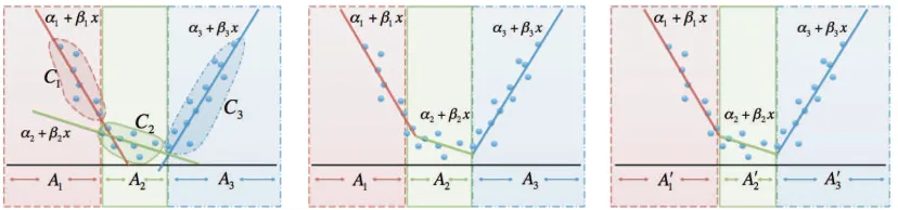
3+3x

A1

1+1x

C 1

C₃

A3

2+2x

A2 C

2

3+3x

A1

1+1x

A3

2+2x

A2

3+3x

A1

1+1x

A3

2+2x

A2

Figure 1: The original space partition A and accompanying data partition C with hyperplanes fit according to that partition (left), the convex estimator based on those hyperplanes; some points are not represented by the hyperplane they were used to fit (center), and subsets refit based on the hyperplanes (right).

previous methods in order to fit piecewise linear maximization functions. Partitions are refined in two steps. First, candidate splits are generated through dyadic splits of existing partitions. These are evaluated and the one that minimizes global error is greedily selected. Second, the new partition is then refit. Although simple, these rules, and refitting in particular, produce large gains over naive adaptive partitioning methods; empirical results are discussed in Section 6.

Most other adaptive partitioning methods use backfitting or pruning to select the tree or partition size. Due to the construction of the CAP estimator, we cannot locally prune and so instead we rely on model selection criteria. We derive a generalized cross-validation method for this setting that is used to select K. This is discussed in Section 5.

3.1 The Algorithm

We now introduce some notation required for convex adaptive partitioning. When presented with data, a partition can be defined over the covariate space (denoted by_{A1, . . . ,AK}, with Ak ⊆

X

or over the observation space (denoted by _{C1, . . . ,CK}, with Ck ⊆ {1, . . . ,n}). The observation

partition is defined from the covariate partition,

Ck={i : xi∈Ak}, k=1, . . . ,K.

The relationship between these is shown in Figure 1. CAP proposes and searches over a set of models, M1, . . . ,MK. A model Mk is defined by: 1) the covariate partition {A1, . . . ,AK}, 2) the

corresponding observation partition, _{C1, . . . ,CK}, and 3) the hyperplanes(αj,βj)Kj=1 fit to those partitions.

The CAP algorithm progressively refines the partition until each subset cannot be split without one subset having fewer than a minimal number of observations, nmin. This value is chosen to

admits logarithmic partition growth,

nmin=min

n

D log(n),2(d+1)

.

Here D is a log scaling factor, which acts to change the base of the log operator. We briefly outline the CAP algorithm below.

3.1.1 CONVEXADAPTIVEPARTITIONING (CAP)

1. Initialize. Set K=1; place all observations into a single observation subset, C1=_{1, . . . ,n}; A1=

X

2. Split. Refine partition by splitting a subset.

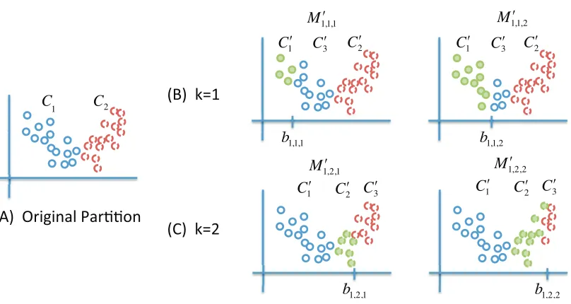
a. Generate candidate splits. Generate candidate model ˆMk jℓby 1) fixing a subset k, 2) fixing a dimension j, 3) dyadically dividing the data in subset k and dimensions j according to knot aℓ. This is done for L knots, all p dimensions and K subsets.

b. Select split. Choose the model MK+1 from the candidates that minimizes global mean squared error on the training set and satisfies mink|Ck| ≥nmin. Set K=K+1.

3. Refit. Use the partition induced by the hyperplanes to generate model M_K′ . Set MK=MK′ if

for every subset C′_kin M_K′ ,_|C_k′_{| ≥}nmin.

4. Stopping conditions. If for every subset Ck in Mk,|Ck|<2nmin, stop fitting and proceed to

step 5. Otherwise, go to step 2.

5. Select model size. Each model Mkcreates an estimator,

fk(x) = max

j∈{1,...,k}αj+β T

jx.

Use generalized cross-validation on the estimators to select final model M∗from_{Mk}K_k=1. 3.2 Splitting Rules

To split, we create a collection of candidate models by splitting a single subset into two subsets. We create models for every subset and search along every cardinal direction by splitting the data along that direction. For a fixed dimension j and subset k, let x_minjk be the minimum value and xmaxjk be the

maximum value of the covariates in this subset and dimension. Let 0<a1<_···<aL<1 be a set

of evenly spaced knots that represent the proportion between x_minjk and xmaxjk .

We create model ˆMjkℓby 1) fixing subset k∈ {1, . . . ,K}, and 2) fixing dimension j∈ {1, . . . ,p}.

x_minjk =min_{xi j : i∈Ck}, xmaxjk =max{xi j : i∈Ck}.

Use the weighted average bjkℓ=aℓxminjk + (1−aℓ)x jk

maxto split Ck and Ak in dimension j. Set

b

1,1,1

C

1 C3 C2

b

1,1,2

C

1 C3 C₂

b

1,2,1

C

1 C2 C3

b

1,2,2

C

1 C2

C

1 C2 C3

M1,1,1 M1,1,2

M1,2,1 M1,2,2

Figure 2: (A) The original observation partition C for M2, (B) new splits generated from the subset C1, and (C) new splits generated from the subset C2. Since there is only one dimension, we fix j=1.

These define new subset and covariate partitions, C′_1:K+1and A′_1:K+1where C_k′′ =Ck′ and Ck′′ =Ck′

for k′₆=k. See Figure 2 for an example. Fit hyperplanes(αˆk,βˆk)K_k=+₁1in each of the subsets. The

triplet of observation partition C_1:K′ ₊₁, covariate partition, A′_1:K+1, and set of hyperplanes(αˆk,βˆk)Kk=+11 defines the model M′_jkℓ. This is done for k=1, . . . ,K, j=1, . . . ,p andℓ=1, . . . ,L. After all models are generated, set K=K+1.

We note that any models where mink|C′k|<nminare discarded. If all models are discarded in

one subset/dimension pair, we produce a model by splitting on the subset median in that dimension.

3.3 Split Selection

We select the model M′_jkℓthat gives the smallest global error. Let(α_ijkℓ,β_ijkℓ)K

i=1be the hyperplanes associated with M′_jkℓand let

ˆ

fjkℓ(x) = max

i∈{1,...,K}α jkℓ

i +β jkℓ

i T

x

be its estimator. We set the model MKto be the one that minimizes global mean squared error,

MK=

( ˆ

Mjkℓ :(j,k, ℓ) =arg min

j,k,ℓ 1 n

n

∑

yi−fˆjkℓ(xi)

2) .

Set ˆfKto be the minimal estimator. We note that MKmay not be unique, however this seldom occurs

3.4 Refitting

We refit by using the partition induced by the hyperplanes. Let (α1:K,β1:K) be the hyperplanes associated with MK. Refit the partitions by

C_k′ =_{xi:αk+βTkxi≥αj+βTjxi,j6=k}

for k=1, . . . ,K. The covariate partition, A′_1:K is defined in a similar manner. Fit hyperplanes in each of those subsets. Let M_K′ be the model generated by the partition C₁′, . . . ,C′_K. Set MK=MK′ if

|C_k′| ≥nminfor all k.

3.5 Stopping Criteria

Stopping criteria are similar to those in tree-based models (Nobel, 1996; Gy¨orfi et al., 2002). That is, the model stops when there are not enough observations within each subset of leaf to generate any further candidate splits,

|Ck| ≤2nmin

for k=1, . . . ,K. After fitting to termination the final model size, however, is chosen through a pruning method discussed Section 5.

3.6 Tunable Parameters

CAP has two tunable parameters, L and nmin. L specifies the number of knots used when generating

candidate models for a split. Its value is tied to the smoothness of f0 and after a certain value, usually 5 to 10 for most functions, higher values of L offer little fitting gain.

We choose a minimal subset size, nmin, that admits at most

O

is used to specify a minimum subset size, nmin=n/(D log(n)). Here D transforms the base of the

logarithm from e into exp(1/D). We have found that D=3 (implying base_≈1.4) is a good choice for most problems.

Increases in either of these parameters increase the computational time. Sensitivity to these parameters, both in terms of predictive error and computational time, is empirically examined in Appendix B.

3.7 Computational Efficiency

Each round of CAP requires

O

4. Consistency

Letting M∗_n be the model for the CAP estimate after n observations, define the discontinuous piecewise linear estimate based on M∗_n,

f_n∗(x) = Kn

∑

αk+βTkx

1_{x∈Ak},

where Knis the partition size, A1, . . . ,AKn are the covariate partitions and(αk,βk) Kn

k=1are the hyper-planes associated with M_n∗. Let fn(x)be the CAP estimator based on M∗_n,

fn(x) = max

k∈{1,...,Kn}

αk+βTkx.

Each subset Ak has an associated diameter, dnk=supx1,x2∈Ak||x1−x2||2. Define the empirical

co-variate mean for subset k as ¯xk= _|C1_k|∑i∈Ckxi.For xi∈Ak,define Γi=

[1, . . . ,1]

d_nk−1(xi₋¯xk)

, Gk=

∑

i∈Ck ΓiΓTi .

Note that(αk,βk) =G−k1∑i∈CkΓiyiwhenever Gkis nonsingular.

Let x1, . . . ,xnbe i.i.d. random variables. We make the following assumptions:

A1.

X

X

A2. There is an a>0 such thatEea|Y−f0(x)|_{|X=xis bounded on}

_X

A3. Letλk be the smallest eigenvalue of|Ck|−1Gk andλn=minkλk. Thenλn remains bounded

away from 0 in probability as n_→∞.

A4. The diameter of the partition maxkd−_nk1_→0 in probability as n_→∞.

A5. The number of observations in each subset satisfies mink=1,...,Kn|Ck|>d−

1

nk

p

n log(n)in prob-ability as n→∞.

Assumptions A1. and A2. place regularity conditions on f0 and the noise distribution, re-spectively. Assumption A3. is a regularity condition on the covariate distribution to ensure the uniqueness of the linear estimates. Assumption A4. is a condition that can be included in the algo-rithm and checked along with the subset cardinality,_|Ck|. If

X

otherwise it can be approximated using_{xi : i_∈Ck}. Assumption A5. ensures that there are enough

observations in the terminal nodes to fit the linear models.

To show consistency of fnunder theℓ∞metric, we first show consistency of fn∗and its derivatives

under theℓ∞metric in Theorem 1. This is similar to Theorem 1 of Chaudhuri et al. (1994) for treed linear models, although we need to modify it to allow partitions with an arbitrarily large number of faces.

Theorem 1 Suppose that assumptions A1. through A5. hold. Then,

max

k=1,...,Kn

sup

x∈Ak

α_k+βT_kx−f₀(x)

→0, max

k=1,...,Kn

sup

x∈Ak

The CAP algorithm is similar to the SUPPORT algorithm of Chaudhuri et al. (1994), except the refitting step of CAP allows partition subsets to be polyhedra with up to Kn faces. Theorem 1 is

analogous to Theorem 1 of Chaudhuri et al. (1994); to prove our theorem, we modify parts of the proof in Chaudhuri et al. (1994) that rely on a fixed number of polyhedral faces. The proof is given in Appendix A.

Using the results from Theorem 1, extension to consistency for fnunder theℓ∞metric is fairly

simple; this is given in Theorem 2.

Theorem 2 Suppose that assumptions A1. through A5. hold. Then,

sup

x∈X|

fn(x)−f0(x)| →0

in probability as n_→∞.

The proof follows immediately from Theorem 1 and some algebra. Details are given in the Ap-pendix A.

5. Generalized Cross-Validation

The terminal model produced by CAP can overfit the data. As a fast approximation to leave-one-out cross-validation, we use generalized cross-validation (GCV) (Golub et al., 1979; Friedman, 1991) to select the best model from all of those produced by CAP, M1, . . . ,MK. A given model MK is

generated by a collection of K linear models. In linear regression, GCV relies on the following approximation

1 n

n

∑

(yi−f−i(xi))2=

1 n

n

∑

yi−fn(xi)

1−Hii

2 ≈1

n

n

∑

yi−fn(xi)

1−Tr(H)

2

, (4)

where Hii is the ith diagonal element of the hat matrix, X(XTX)−1XT, ˆf₋i is the estimator

condi-tioned on all of the data minus element i. We note that Tr(H)is sometimes approximated by the degrees of freedom divided by the number of observations.

The model MK is defined by C1, . . . ,CK, the partition, and the hyperplanes(αk,βk)K_k=1, which

were generated by the partition. Let (α(_k−i),β(_k−i))K

k=1 be the collection of hyperplanes generated when observation i is removed; notice that if i∈Ck, only(αk,βk)changes. Let ˆf−iKbe the estimator

for model MKwith observation i removed. Using the derivation in Equation (4),

1 n

n

∑

yi−fˆ₋iK(xi)

2

= 1

n

n

∑

yi− max k∈{1,...,K}α

(−i)

k +β

(−i)

k T xi 2 , = 1 n n

∑





yi−αk(i)−βTk(i)xi

1₋H_iik(i)1_{i_∈Ck(i)}



 2

≈ 1_n

n

∑

yi−αk(i)−βTk(i)xi

1₋Tr(Hk(i)₎₁

{i∈Ck(i)}

!2

Number of Observations

4 5 6 7 8 9

0.5 1.0 1.5 2.0

200 400 600 800 1000

100 500 1000 5000

K

MSE

T

ime

Algorithm

GCV

5Fold CV

10Fold CV

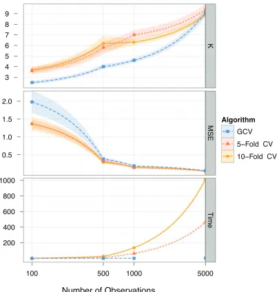
Figure 3: Log-continuous plots for number of observations vs. K (top), MSE (middle), and run-time in seconds (bottom) for GCV, 5-fold and 10-fold cross validation, plus/minus one standard error. Data were generated from 10 i.i.d. training sets with x_∼N5(0,I), y= (x1+.5x2+x3)2₋x4+.25x2₅+ε,andε_∼N(0,1).

where, in a slight abuse of notation, H_iik is the diagonal entry of the hat matrix for subset k corre-sponding to element i, and

k(i) =arg max

k∈{1,...,K}

αk+βTkxi

1₋Tr(Hk₎₁ {i_∈Ck}

To select K, we find the K that minimizes the right hand side of Equation (5). Although more computationally intensive than GCV in linear models, the computational complexity for CAP GCV is similar to that of the CAP split selection step.

We empirically compared GCV selection of K with 5- and 10-fold cross validation selection of K. GCV tends to select a smaller K than full cross validation, particularly on smaller problems. Predictive results, however, are comparable for moderate to large problem sizes (n_≥5,000) while the runtime of GCV is orders of magnitude less than 5- and 10-fold cross validation. We should expect more discrepancy between cross-validation and GCV on smaller problems because GCV relies on an asymptotic approximation. In these cases, full cross validation selection of K may be worthwhile. Representative results are given in Figure 3.

We can use generalized cross-validation to create a more efficient stopping rule for CAP. We note that GCV scores are often unimodal in K. Instead of fully growing the tree, we stop splitting after the score has increased twice in a row. The resulting algorithm is called Fast CAP; details are given in Appendix B.

6. Empirical Analysis

We compare shape constrained and unconstrained regression methods across a set of convex re-gression problems: two synthetic rere-gression problems, predicting mean weekly wages and value function approximation for pricing basket options.

6.1 Synthetic Regression Problems

We apply CAP to two synthetic regression problems to demonstrate predictive performance and analyze sensitivity to tunable parameters. The first problem has a non-additive structure, high levels of covariate interaction and moderate noise, while the second has a simple univariate structure em-bedded in a higher dimensional space and low noise. Low noise or noise free problems often occur when a highly complicated convex function needs to be approximated by a simpler one (Magnani and Boyd, 2009).

6.1.1 PROBLEM1

Here x_∈R5. Set

y= (x1+.5x2+x3)2₋x4+.25x2₅+ε,

whereε_∼N(0,1). The covariates are drawn from a 5 dimensional standard Gaussian distribution, N5(0,I).

6.1.2 PROBLEM2

Here x_∈R10. Set

y=exp xTq+ε,

where q was randomly drawn from a Dirichlet(1,. . .,1) distribution,

q= (0.0680,0.0160,0.1707,0.1513,0.1790,0.2097,0.0548,0.0337,0.0377,0.0791)T.

6.1.3 PREDICTIVEPERFORMANCE ANDRUNTIMES

We compared the performance of CAP and Fast CAP to other regression methods on problems 1 and 2. We implemented the following shape constrained algorithms: the least squares regression (LSE) usingcvx (Grant and Boyd, 2012, 2008), and the linear refitting algorithm of Magnani and Boyd (2009). The general methods included Gaussian processes (Rasmussen and Williams, 2006) using

gpmlin Matlab, tree regression with constant values in the leaves usingclassregtreein Matlab, multivariate adaptive regression splines (MARS) (Friedman, 1991) usingARESlabin Matlab, and support vector machines (SVMs) using thee1071package inR.

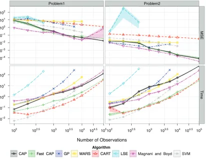
For CAP and Fast CAP, we set the parameters to D=3 and L=10; the sensitivity to these parameters is examined in Appendix C. The parameter K was chosen by GCV for CAP. In Fast CAP, the number of random search directions was set to be p=min(d,10). All methods were given a maximum runtime of 90 minutes, after which the results were discarded. Methods were run on 10 random training sets and tested on the same testing set of 10,000 random covariates. Average runtimes and predictive performance are shown in Figure 4.

Non-convex regression methods performed poorly compared to shape restricted methods, par-ticularly in the higher noise setting. Amongst the shape restricted methods, only CAP and Fast CAP had consistently low predictive error. The method of Magnani and Boyd (2009) can become unstable, which is seen in problem 1. Surprisingly, the LSE had high predictive error. This can be attributed to overfitting, particularly in the boundary regions. A demonstration is given in Figure 5. Although CAP and Fast CAP had similar predictive performance, their runtimes often differed by an order of magnitude with the largest differences on the biggest problem sizes. Based on this performance, we would suggest using Fast CAP on larger problems.

We note that the empirical rate of convergence for CAP and Fast CAP is much faster than would be predicted by minimax convergence rates. The results, however, are consistent with rates that adapt to an underlying linear subspace; this is examined in Appendix D.

6.1.4 CAP ANDTREEDLINEARMODELS

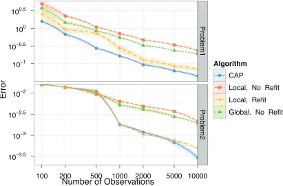
Treed linear models are a popular method for regression and classification. They can be easily modified to produce a convex regression estimator by taking the maximum over the linear leaves. CAP differs from existing treed linear models in how the partition is refined. First, subset splits are selected based on global reduction of error. Second, the partition is refit after a split is made. To investigate the contributions of each step, we compare to treed linear models generated by: 1) local error reduction as an objective for split selection and no refitting, 2) global error reduction as an objective function for split selection and no refitting, and 3) local error reduction as an objective for split selection along with refitting. All estimators based on treed linear models are generated by taking the maximum over the set of linear models in the leaves. We compared the performance of these methods on problems 1 and 2 over 10 different training sets and a single testing set. Average predictive error is displayed in Figure 6.

Number of Observations

104

103

102

101

100

101

102

102

101

100

101

102

Problem1

102 102.5 103 103.5 104 104.5 105

Problem2

102 102.5 103 103.5 104 104.5 105

MSE

T

ime

Algorithm

CAP Fast CAP GP MARS CART LSE Magnani and Boyd SVM

Figure 4: Mean squared error (top) and runtime in seconds (bottom) plus/minus one standard error on problem 1 (left) and problem 2 (right) for CAP, Fast CAP, Gaussian processes, MARS, CART, the least squares estimator, the linear fitting method of Magnani and Boyd (2009) and support vector machines.

6.2 Predicting Weekly Wages

We use shape restricted methods to predict mean weekly wages based on years of education and experience. The data are from the 1988 Current Population Survey (CPS); they originally appeared in Bierens and Ginther (2001) and can be accessed as ex1029in theSleuth2 package inR. The data set contains 25,361 records of weekly wages for full-time, adult, male workers for 1987, along with years experience, years of education, race (either back or white; no others were included in the sample), region, and whether the last job held was part time.

1 0.5

0 0.5

1

1 0

1 0 1 2

CAP (A)

1 0.5

0 0.5

1

1 0

1 0 1 2

Least Squares Estimator (B)

Figure 5: (A) The CAP estimator, and (B) the LSE fit to 500 observations drawn from y=x2₁+

x2

2+ε,whereε∼N(0,0.252). The covariates were drawn from a 2 dimensional uniform distribution, Unif[₋1,1]2_{. The LSE was truncated at predicted values of 2.5 for display,} although some predicted values reached as high as 4,800 on[₋1,1]2_.

Number of Observations

E

rr

o

r

101

100.5

100

100.5

103.5

103

102.5

102

100 200 500 1000 2000 5000 10000

P

ro

b

le

m

1

P

ro

b

le

m

2

Algorithm

_CAP

Local, No Refit

Local, Refit

Global, No Refit

Years Experience M e a n W e e k ly W a g e 200 300 400 500 600 700

0 10 20 30 40 50 60

Years Education M e a n W e e k ly W a g e 400 500 600 700 800 900

0 5 10 15

1.2^Years Education M e a n W e e k ly W a g e 400 500 600 700 800 900

5 10 15 20 25

Figure 7: Mean weekly wages vs. years of experience (left), mean weekly wages vs. years of education (center), mean weekly wages vs. 1.2years education(right).

R o o t M e a n Sq u a re d Er ro r 300 350 400 450 500 550 600 650

CAP CART FastCAP MARS SVM

method CAP CART FastCAP MARS SVM R u n ti m e ( in se c o n d s ) 50 100 150

CAP CART FastCAP MARS SVM method CAP CART FastCAP MARS SVM

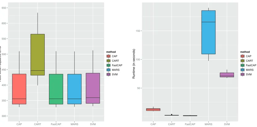
Figure 8: Root mean squared error (RMSE), left, and runtime in seconds, right, for CAP, Fast CAP, CART, MARS, and SVMs for predicting weekly wages based on years experience and years education.

1.2years education, as a covariate. Shape restrictions do not hold with any other covariates, so they are discarded.

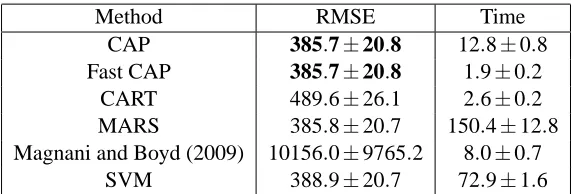
Method RMSE Time CAP 385.7_±20.8 12.8_±0.8 Fast CAP 385.7_±20.8 1.9_±0.2

CART 489.6±26.1 2.6±0.2 MARS 385.8_±20.7 150.4_±12.8 Magnani and Boyd (2009) 10156.0_±9765.2 8.0_±0.7

SVM 388.9_±20.7 72.9_±1.6

Table 1: Average RMSE and runtime in seconds, plus/minus one standard error for CAP, Fast CAP, CART, MARS, Magnani and Boyd (2009) and SVMs.

This data set presents difficulties for many methods due to its size (n>20,000) and highly skewed distribution. CAP, Fast CAP, MARS and SVMs all had comparable predictive error rates, while CART produced error rates about 27% higher. The linear fitting method of Magnani and Boyd (2009) occasionally tried to fit outliers with hyperplanes, resulting in about a 2,500% increase in predictive error. This potential instability is one of the largest drawbacks with the method of Magnani and Boyd (2009). In terms of runtimes, Fast CAP and CAP were both significantly faster than any methods that produced comparable results, with runtime reductions of more than 80% over SVMs.

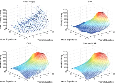
In Figure 9, we compare the predicted functions produced by CAP and SVMs. In areas with small amounts of data, such for people with low education, the SVM produces results that do not match prior information. In the SVM surface, someone with 0 years of experience and 0 years of education is predicted to have about a 150% larger weekly wage than a high school graduate with 0 years of experience and about the same weekly wage as someone with a 4-year college degree and 0 years of experience. By imposing shape constraints, CAP eliminates these types of problems and produces a surface that conforms to prior knowledge.

Unlike the surface produced by SVM regression, the surface produced by CAP is not smooth. A greater degree of smoothness can be added through ensemble methods like bagging (Breiman, 1996) and smearing (Breiman, 2000). Averaging randomized convex estimators produces a new convex estimator; these methods have been explored for approximating objective functions in Hannah and Dunson (2012). A surface produced by smearing CAP is shown on the right in Figure 9. Note that its overall shape is quite similar to the original CAP estimator while most of the sharp edges have been smoothed away.

6.3 Pricing Stock Options

In sequential decision problems, a decision maker takes an action based on a currently observed state of the world based on the current rewards of that action and possible future rewards. Approximate dynamic programming is a modeling method for such problems based on approximating a value-to-go function. Value-to-value-to-go functions, or simply “value functions,” give the value for each state of the world if all optimal decisions are made subsequently.

0 5 10 15 20 0 20 40 60 800 200 400 600 800 1000 1200 M e a n We e k ly S a la ry Mean Wages Years Education

Years Experience 0 5

10 15 20 0 20 40 60 800 200 400 600 800 1000 1200 Years Education SVM Years Experience We e k ly S a la ry 0 5 10 15 20 0 20 40 60 800 200 400 600 800 1000 1200 Years Education CAP Years Experience We e k ly S a la ry 0 5 10 15 20 0 20 40 60 800 200 400 600 800 1000 1200 Years Education Smeared CAP Years Experience We e k ly S a la ry

Figure 9: Mean weekly wage based on years of experience and years of education (top left), pre-dicted values using SVM regression (top right), CAP (bottom left), and smeared CAP (bottom right).

required for computational tractability. Convex regression holds great promise for value function approximation in these problems.

To give a simple example for value function approximation, we consider pricing American basket options on the average of M underlying assets. Options give the holder the right—but not the obligation—to buy the underlying asset, in this case the average of M individual assets, for a predetermined strike price R. In an American option, this can be done at any time between the issue date and the maturity date, T . However, American options are notoriously difficult to price, particularly when the underlying asset base is large.

A popular method for pricing American options uses approximate dynamic programming where continuation values are approximated via regression (Carriere, 1996; Tsitsiklis and Van Roy, 1999, 2001; Longstaff and Schwartz, 2001). We summarize these methods as follows; see Glasserman (2004) for a more thorough treatment. The underlying assets are assumed to have the sample path {X1, . . . ,XT}, where Xt ={S1(t), . . . ,SM(t)} is the set of securities at time t. At each time t, a

continuation value function, ¯Vt(Xt), is estimated by regressing a value function for the next time

period, ¯Vt+1(Xt+1), on the current state, Xt. The continuation value is the value of holding the

be the max of the current exercise value and the continuation value. Options are exercised when the current exercise value is greater than or equal to the continuation value.

The procedure to estimate the continuation values is as follows (as summarized in Glasserman 2004):

0. Define basket payoff function,

h(Xt) =max

( 1 M

M

∑

Sk(t)₋R,0 )

.

1. Sample N independent paths,_{X1 j, . . . ,XT j}, j=1, . . . ,N.

2. At time T , set ¯VT(XT j) =h(XT j).

3. Apply backwards induction: for t=T₋1, . . . ,1,

• given _{V¯t+1(Xt+1 j)}N_j=1, regress on {Xt j}N_j=1 to get continuation value estimates

{_C¯_{t(Xt j)}}N j=1. • set value function,

¯

Vt(Xt j) =maxh(Xt j),C¯t(Xt j) .

We use the value function defined by Tsitsiklis and Van Roy (1999).

The regression values are used to create a policy that is implemented on a test set: exercise when the current exercise value is greater than or equal to the estimated continuation value. A good regression model is crucial to creating a good policy.

In previous literature,_{Ct(Xt j)}N_j=1has been estimated by regression splines for a single

under-lying asset (Carriere, 1996), or least squares linear regression on a set of basis functions (Tsitsiklis and Van Roy, 1999; Longstaff and Schwartz, 2001; Glasserman, 2004). Regression on a set of ba-sis functions becomes problematic when Xt j is defined over moderate to high dimensional spaces.

Well-defined sets of bases such as radial basis functions and polynomials require an exponential number of functions to span the space, while manually selecting basis functions can be quite diffi-cult. Since the expected continuation values are convex in the asset price for basket options, CAP is a simple, nonparametric alternative to these methods.

We compared the following methods: CAP and Fast CAP with D=3, L=10 for both and P′=min(M,10), the number of random search directions in Fast CAP; the method of Magnani and Boyd (2009); regression trees with constant leaves using the Matlab functionclassregtree; least squares using the polynomial basis functions

(1,Si(t),Si2(t),S3i(t),Si(t)Sj(t),h(Xt)), i=1, . . . ,M, j6=i;

ridge regression on the same basis functions with ridge parameter chosen by 10-fold cross-validation each time period from values between 10−3_{and 10}5_.

was generated using the dual martingale methods of Haugh and Kogan (2004) from value functions generated using polynomial basis functions based on the mean of the assets,(1,Yt,Yt2,Yt3,h(Yt)),

where Yt =1/M∑iM=1Xi(t), with 2,000 samples. Upper and lower bounds were generated using 5

training and testing sets.

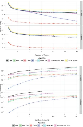
Results are displayed in Figure 10. We found that CAP and Fast CAP gave state of the art per-formance without the difficulties associated with linear functions, such as choosing basis functions and regularization parameters. We observed a decline in the performance of least squares as the number of assets grew due to overfitting. Ridge regularization greatly improved the least squares performance as the number of assets grew. Tree regression did poorly in all settings, likely due to overfitting in the presence of the non-symmetric error distribution generated by the geometric Brownian motion. These results suggest that CAP is robust even in less than ideal conditions, such as when data have heteroscedastic, non-symmetric error distributions.

Again, we noticed that while the performances of CAP and Fast CAP were comparable, the runtimes were about an order of magnitude different. On the larger problems, runtimes for Fast CAP were similar to those for unregularized least squares. This is likely because the number of covariates in the least squares regression grew like M2, while all linear regressions in CAP only had M covariates.

7. Conclusions

In this article, we presented convex adaptive partitioning, a computationally efficient, theoretically sound and empirically robust method for regression subject to a convexity constraint. CAP is the first convex regression method to scale to large problems, both in terms of dimensions and number of observations. As such, we believe that it can allow the study of problems that were once thought to be computationally intractable. These include econometrics problems, like estimating consumer preference or production functions in multiple dimensions, approximating complex constraint func-tions for convex optimization, or creating convex value-to-go funcfunc-tions or response surfaces that can be easily searched in stochastic optimization.

Number of Assets

V

a

lu

e

o

f

P

o

lic

y

5 10 15 20 25

5 10 15 20 25

5 10 15 20 25 30

n

=

1

0

0

0

0

n

=

5

0

0

0

0

Algorithm

CAP Fast CAP CART LS Ridge LS Magnani and Boyd Upper Bound

Number of Assets

Ti

m

e

(

in

s

e

c

o

n

d

s

)100

101

102

103

100

101

102

103

104

5 10 15 20 25 30

n

=

1

0

0

0

0

n

=

5

0

0

0

0

Algorithm

CAP Fast CAP CART LS Ridge LS Magnani and Boyd

8. Online Supplements

Code for CAP can be downloaded athttp://www.columbia.edu/˜lah2178/Research.htmland as an online supplement at the JMLR website.

Acknowledgments

This work was partially supported by grant R01 ES017240 from the National Institute of Environ-mental Health Sciences (NIEHS) of the National Institutes of Health (NIH). Lauren A. Hannah was partially supported by the Provost’s Postdoctoral Fellowship at Duke University.

Appendix A.

The proof of Theorem 1 is essentially identical to the proof of Theorem 1 of Chaudhuri et al. (1994) with a few modifications. The Chaudhuri et al. (1994) results are for an algorithm that splits subsections parallel to axes. By allowing subsets to be determined by the dominating hyperplanes, the subsets are now polyhedral with a maximal number of faces determined by the dimension and maximal number of subsets. To show this, we modify Lemma 12.27 of Breiman et al. (1984).

Proof [Proof of Theorem 1] It is sufficient to show that

max

k=1,...,Kn

d_nk−1[α_k,βk]t−∆(¯xk) →0

in probability, where∆(¯xk) is the vector of elements[f0(x¯k,dnk−1∂∂x1f0(¯xk), . . . ,d

−1

nk ∂∂xp f0(¯xk)] t_{. Let}

α0

k =αk−βtk¯xk. Assumption A3. ensures that the matrices Dk for all subsets are nonsingular with

probability tending to 1, where Dk=∑xi∈CkΓiΓ t

i. Letting Yi= f0(xi) +εi, we have [α0_k,βk]t=D−_k1

∑

xi∈Ck

Γif0(xi) +D−_k1

∑

xi∈Ck

Γiεi (6)

for k=1, . . . ,Knwith probability tending towards 1. Doing a Taylor expansion of Equation (6), we

get

[α0_k,βk]t−∆(¯xk) =D−k1

∑

Γir(xi−¯xk) +D−k1

∑

Γiεi,

where r(xi₋¯xk)are the second order and above terms of the Taylor expansion of f0(¯xk).

Assump-tions A1., A3. and A4. ensure maxk=1,...,Kn

d−_nk1D−_k1∑_i∈C

kΓir(xi−¯xk)

→0 in probability as n→∞. To bound the random error term of Equation (6), we first assume that Ak is fixed. Applying Lemma

12.26 of Breiman et al. (1984) to each component of d_nk−1|Ck|−1∑i∈CkΓiεi, there exist constants

h1>0, h2>0 andγ0>0 such that

P d_nk−1

|Ck|−1

∑

Γiεi

>γ !

≤h1e−h2d

2

nk|Ck|γ2_{, (7)}

Kn(p+2). Following the proof of 12.27, for mn such that mn/log(n)→∞, we use Equation (7) to

show

P [α0_k,β_k]t−∆(¯x_k)

≥γ|x_1:n

≤h1e−h2γ

2_nd2

nk|Ck|/n_,

≤h1e−h2γ2mnlog(n)_, =h1n−h2γ2mn

on the event d2_nk|Ck|/n≥mnlog(n)/n. Using the VC dimension of the partition,

P [α0_k,βk]t−∆(¯xk)

≥γfor each A_kand d_nk2|C_k| ≥m_nD log(n)

≤h121+Kn(p+2)_nKn(p+2)−h2γ2mn_.

Since A5. ensures that mn→∞, the result holds.

Proof [Proof of Theorem 2] Fixε>0; let dX be the diameter of

X

n_≥N

P (

max

k=1,...,Kn

sup

x∈Ak

α_k+βT_kx−f0(x) >

ε ζdX

) <ε/2,

P (

max

k=1,...,Kn

sup

x∈Ak

||βk−∇f0(x)||_∞>

ε ζdX

) <ε/2.

Fix aδnet over

X

P

sup

x∈X|

fn(x)−f0(x)|>ε

=P

sup

x∈X

max

k=1,...,Kn

αk+βTkx−f0(x) >ε , ≤P max

i=1,...,nδ

max

k=1,...,Kn

αk+βTkxδi −f0(xδi)

> ε ζ , ≤P ( max

i=1,...,nδ

Kn

∑

αk+βTkxδi

1_{xδ

i∈Ak}−f0(x δ i) > ε ζdX

) ,

<ε.

Appendix B.

To alleviate the first problem, we suggest using P′ random projections as a basis for search. Using ideas similar to compressive sensing, each projection gj∼Np(0,I)for j=1, . . . ,P′. Then we

search along the direction gT_jx rather than xj. When we expect the true function to live in a lower

dimensional space, as is the case with superfluous covariates, we can set P′<p.

We solve the second problem by modifying the stopping rule. Instead of fully growing the tree until each subset has less than 2n/(2 log(n))observations, we use generalized cross-validation. We grow the tree until the generalized cross-validation value has increased in two consecutive iterations or each subset has less than 2n/(2 log(n))observations. As the generalized cross-validation error is usually concave in K, this heuristic often offers a good fit at a fraction of the computational expense of the full CAP algorithm.

The Fast CAP algorithm has the potential to substantially reduce the log(n)2_{factor by halting} the model generation long before K reaches D log(n). Since every feasible partition is searched for splitting, the computational complexity grows as k gets larger.

The Fast CAP algorithm is summarized as follows.

B.1 Fast Convex Adaptive Partitioning (Fast CAP)

1. Initialize. As in CAP.

2. Split.

a. Generate candidate splits. Generate candidate model ˆMjkℓ by 1) fixing a subset k, 2) generating a random direction j with gj∼Np(0,I), and 3) dividing the data as follows:

• set x_minjk =min{gT_jxi: i∈Ck}, xmaxjk =max{gTjxi: i∈Ck}and bjkℓ=aℓxminjk + (1−

aℓ)xmaxjk

• set

C_k′ =_{i : i_∈Ck,gTjxi≤bjkℓ}, CK′+1={i : i∈Ck,gTjxi>bjkℓ}, A′_k=_{x : x_∈Ak,gTjx≤bjkℓ}, A′K+1={x : x∈Ak,gTjx>bjkℓ}. Then new hyperplanes are fit to each of the new subsets. This is done for L knots, P′ dimensions and K subsets.

b. Select split. As in CAP.

3. Refit. As in CAP.

4. Stopping conditions. Let GCV(MK)be the generalized cross-validation error for model MK.

Stop if GCV(MK) >GCV(MK−1) and GCV(MK−1)>GCV(MK−2) of if |Ck|<2nmin for

k=1, . . . ,K. Then select final model as in CAP.

Appendix C.

In this subsection, we empirically examine the effects of the two tunable parameters, the log factor, D, and the number of knots, L. The log factor controls the minimal number of elements in each subset by setting_|Ck| ≥n/(D log(n)), and hence it controls the number of subsets, K, at least for

D

103 102 101 100 101

103 102 101 100 101 102

Problem1

1 3 5 10 20

Problem2

1 3 5 10 20

MSE

T

im

e

(s

e

c

o

n

d

s

)

Algorithm

CAP, n=500 Fast CAP, n=500 CAP, n=5,000 Fast CAP, n=5,000

Figure 11: Log factor D (log scale) vs. mean squared error (log scale) for CAP and Fast CAP (top). Log factor D (log scale) vs. runtime in seconds (log scale) (bottom). Both methods were run on problem 1 (left) and problem 2 (right) with n=500 and n=5,000. Lines are mean value and shading represents one standard error.

cost of greater computational time due to the increase in possible values for K and the larger number of possibly admissible sets generated in the splitting step of CAP.

We compared values for D ranging from 0.1 to 20 on problems 1 and 2 with sample sizes of n=500 and n=5,000 over 100 training sets and one testing set. Results are displayed in Figure 11. Note that error may not be strictly decreasing with D because different subsets are proposed under each value. Additionally, Fast CAP is a randomized algorithm so variance in error rate and runtime is to be expected.

Empirically, once D _≥1, there was little substantive error reduction in the models, but the runtime increased as

O

L

102.5 102 101.5 101 100.5

101.5 101 100.5 100 100.5 101 101.5

Problem1

1 2 3 5 10 1520 50

Problem2

1 2 3 5 10 1520 50

MSE

T

im

e

(s

e

c

o

n

d

s

)

Algorithm

_{CAP, n=500 Fast CAP, n=500 CAP, n=5,000 Fast CAP, n=5,000}

Figure 12: Number of knots L (log scale) vs. mean squared error (log scale) for CAP and Fast CAP (top). Number of knots L (log scale) vs. runtime in seconds (log scale) (bottom). Both methods were run on problem 1 (left) and problem 2 (right) with n=500 and n=5,000. Lines are mean value and shading represents one standard error.

on these results, we believe that setting D=3 offers a good balance between fit and computational expense.

The number of knots, L, determines how many possible subsets will be examined during the splitting step. Like D, an increase in L offers a better fit at the expense of increased computation. We compared values for L ranging from 1 to 50 on problems 1 and 2 with sample sizes of n=500 and n=5,000 over 100 training sets and 1 testing set. Results are displayed in Figure 12.

103 104 105 101

100

Number of Observations

(A)

S

q

rt

(M

e

a

n

S

q

u

a

re

d

E

rr

o

r)

CAP Fast CAP CAP Fit Fast CAP Fit

103 104 105

102 101

Number of Observations

(B)

CAP Fast CAP CAP Fit Fast CAP Fit

Figure 13: Number of observations n (log scale) vs. square root of mean squared error (log scale) for problem 1 (A) and problem 2 (B). Linear models are fit to find the empirical rate of convergence.

Appendix D.

Although theoretical rates of convergence are not yet available for CAP, we are able to empirically examine them. Rates of convergence for multivariate convex regression have only been studied in two articles of which we are aware. Aguilera et al. (2011) studied rates of convergence for an estimator that is created by first smoothing the data, then evaluating the smoothed data over anε-net, and finally convexifying the net of smoothed data by taking the convex hull. They showed that the convexify step preserved the rates of the smoothing step. For most smoothing algorithms, these are minimax nonparametric rates, n−p+21 _{with respect to the empiricalℓ}

2norm.

Hannah and Dunson (2011) showed adaptive rates for a Bayesian model that places a prior over the set of all piecewise linear functions. Specifically, they showed that if the true mean function f0 actually maps a d-dimensional linear subspace of

X

f0(x) =g0(xA), A∈Rp×d,

then their model achieves rates of log−1(n)n−d+21 _{with respect to the empirical}ℓ_{2norm. Empirically,}

we see these types of adaptive rates with CAP.

Method Problem 1 Problem 2 Expected: Rates in p ₋0.1429 ₋0.0833 Expected: Rates in d ₋0.2000 ₋0.3333 Empirical: CAP ₋0.2003 ₋0.2919 Empirical: Fast CAP ₋0.2234 ₋0.2969

Table 2: Slopes for linear models fit to log(n) vs. log(√MSE) in Figure 13. Expected slopes are given when: 1) rates are with respect to full dimensionality, p, and 2) rates are with respect to dimensionality of linear subspace, d. Empirical slopes are fit to mean squared error generated by CAP and Fast CAP. Note that all empirical slopes are closest to those for linear subspace rates rather than those for full dimensionality rates.

in Table 2. These results strongly imply that CAP achieves adaptive convergence rates of the type shown by Hannah and Dunson (2011) for problems 1 and 2.

References

N´estor Aguilera and Pedro Morin. Approximating optimization problems over convex functions. Numerische Mathematik, 111(1):1–34, 2008.

N´estor Aguilera and Pedro Morin. On convex functions and the finite element method. SIAM Journal on Numerical Analysis, 47(1):3139–3157, 2009.

N´estor Aguilera, Liliana Forzani, and Pedro Morin. On uniform consistent estimators for convex regression. Journal of Nonparametric Statistics, 23(4):897–908, 2011.

Yacine A¯ıt-Sahalia and Jefferson Duarte. Nonparametric option pricing under shape restrictions. Journal of Econometrics, 116(1–2):9–47, 2003.

William P. Alexander and Scott D. Grimshaw. Treed regression. Journal of Computational and Graphical Statistics, 5(2):156–175, 1996.

Gad Allon, Michael Beenstock, Steven Hackman, Ury Passy, and Alexander Shapiro. Nonpara-metric estimation of concave production technologies by entropic methods. Journal of Applied Econometrics, 22(4):795–816, 2007.

Herman J. Bierens and Donna K. Ginther. Integrated conditional moment testing of quantile regres-sion models. Empirical Economics, 26(1):307–324, 2001.

Melanie Birke and Holger Dette. Estimating a convex function in nonparametric regression. Scan-dinavian Journal of Statistics, 34(2):384–404, 2007.

Stephen Boyd and Lieven Vandenberghe. Convex Optimization. Cambridge University Press, Cam-bridge, United Kingdom, 2004.