How to Solve Classification and Regression Problems on
High-Dimensional Data with a Supervised
Extension of Slow Feature Analysis
Alberto N. Escalante-B. [email protected]
Laurenz Wiskott [email protected]
Institut f¨ur Neuroinformatik Ruhr-Universit¨at Bochum Bochum D-44801, Germany
Editor:David Dunson
Abstract
Supervised learning from high-dimensional data, for example, multimedia data, is a challenging task. We propose an extension of slow feature analysis (SFA) forsuperviseddimensionality reduc-tion called graph-based SFA (GSFA). The algorithm extracts a label-predictive low-dimensional set of features that can be post-processed by typical supervised algorithms to generate the final label or class estimation. GSFA is trained with a so-called training graph, in which the vertices are the samples and the edges represent similarities of the corresponding labels. A new weighted SFA op-timization problem is introduced, generalizing the notion of slowness from sequences of samples to such training graphs. We show that GSFA computes an optimal solution to this problem in the considered function space and propose several types of training graphs. For classification, the most straightforward graph yields features equivalent to those of (nonlinear) Fisher discriminant anal-ysis. Emphasis is on regression, where four different graphs were evaluated experimentally with a subproblem of face detection on photographs. The method proposed is promising particularly when linear models are insufficient as well as when feature selection is difficult.
Keywords: slow feature analysis, feature extraction, classification, regression, pattern recogni-tion, training graphs, nonlinear dimensionality reducrecogni-tion, supervised learning, implicitly super-vised, high-dimensional data, image analysis
1. Introduction
Supervised learning from high-dimensional data has important applications in areas such as multi-media processing, human-computer interfaces, industrial quality control, speech processing, robotics, bioinformatics, image understanding, and medicine. Despite constant improvements in computa-tional resources and learning algorithms, supervised processing, for example, for regression or clas-sification, of high-dimensional data is still a challenge largely due to insufficient data and several phenomena referred to as the curse of dimensionality. This limits the practical applicability of supervised learning.
However, since the final goal is to solve a supervised learning problem, this approach is inherently suboptimal.
Supervised dimensionality reduction is more appropriate in this case. Its goal is to compute a low-dimensional set of features from the high-dimensional input samples that contains predictive information about the labels (Rish et al., 2008). One advantage is that dimensions irrelevant for the label estimation can be discarded, resulting in a more compact representation and more accu-rate label estimations. Different supervised algorithms can then be applied to the low-dimensional data. A widely known algorithm for supervised dimensionality reduction is Fisher discriminant analysis (FDA) (Fisher, 1936). Sugiyama (2006) proposed local FDA (LFDA), an adaptation of FDA with a discriminative objective function that also preserves the local structure of the input data. Later, Sugiyama et al. (2010) proposed semi-supervised LFDA (SELF) bridging LFDA and PCA and allowing the combination of labeled and unlabeled data. Tang and Zhong (2007) in-troduced pairwise constraints-guided feature projection (PCGFP), where two types of constraints are allowed. Must-link constraints denote that a pair of samples should be mapped closely in the low-dimensional space, while cannot-link constraints require that the samples are mapped far apart. Later, Zhang et al. (2007) proposed semi-supervised dimensionality reduction (SSDR), which is similar to PCGFP and also supports semi-supervised learning.
Slow feature analysis (SFA) (Wiskott, 1998; Wiskott and Sejnowski, 2002) is an unsupervised learning algorithm inspired by the visual system and based on the slowness principle. SFA has been applied to classification in various ways. Franzius et al. (2008) extracted the identity of animated fish invariant to pose (including a rotation angle and the fish position) with SFA. A long sequence of fish images was rendered from 3D models in which the pose of the fish changed following a Brown-ian motion, and in which the probability of randomly changing the fish identity was relatively small, making identity a feature that changes slowly. This result confirms that SFA is capable of extracting categorical information. Klampfl and Maass (2010) introduced a particular Markov chain to gen-erate a sequence used to train SFA for classification. The transition probability between samples from different object identities was proportional to a small parametera. The authors showed that in the limita→0 (i.e., only intra-class transitions), the features learned by SFA are equivalent to the features learned by Fisher discriminant analysis (FDA). The equivalence of the discrimination capability of SFA and FDA in some setups was already known (compare Berkes, 2005a, and Berkes, 2005b) but had not been rigorously shown before. In the two papers by Berkes, hand-written digits from the MNIST database were recognized. Several mini-sequences of two samples from the same digit were used to train SFA. The same approach was also applied more recently to human gesture recognition by Koch et al. (2010) and a similar approach to monocular road segmentation by Kuhnl et al. (2011). Zhang and Tao (2012) proposed an elaborate system for human action recognition, in which the difference between delta values of different training signals was amplified and used for discrimination.
SFA has been used to solve regression problems as well. Franzius et al. (2008) used standard SFA to learn the position of animated fish from images with homogeneous background. The same training sequence used for learning fish identities was used, thus the fish position changed continu-ously over time. However, a different supervised post-processing step was employed consisting of linear regression coupled with a nonlinear transformation.
SFA problem, generalizing the concept of signal slowness. The objective function of the GSFA problem is a weighted sum of squared output differences and is therefore similar to the underlying objective functions of, for example, FDA, LFDA, SELF, PCGFP, and SSDR. However, in general the optimization problem solved by GSFA differs at least in one of the following elements: a) the concrete coefficients of the objective function, b) the constraints, or c) the feature space consid-ered. Although nonlinear or kernelized versions of the algorithms above can be defined, one has to overcome the difficulty of finding a good nonlinearity or kernel. In contrast, SFA (and GSFA) was conceived from the beginning as a nonlinear algorithm without resorting to kernels (although there exist versions with a kernel: Bray and Martinez, 2003; Vollgraf and Obermayer, 2006; B¨ohmer et al., 2012), with linear SFA being just a less used special case. Another difference to various algo-rithms above is that SFA (and GSFA) does not explicitly attempt to preserve the spatial structure of the input data. Instead, it preserves the similarity structure provided, which leaves room for better optimization towards the labels.
Besides the similarities and differences outlined above, GSFA is strongly connected to some algorithms in specific cases. For instance, features equivalent to those of FDA can be obtained if a particular training graph is given to GSFA. There is also a close relation between SFA and Laplacian eigenmaps (LE), which has been studied by Sprekeler (2011). GSFA and LE basically have the same objective function, but in general GSFA uses different edge-weight (adjacency) matrices, has different normalization constraints, supports node-weights, and uses function spaces.
There is also a strong connection between GSFA and LPP. In Section 7.1 we show how to use GSFA to extract LPP features andvice versa. This is a remarkable connection because GSFA and LPP originate from different backgrounds and are typically used for related but different goals. Generalized SFA (Sprekeler, 2011; Rehn, 2013), being basically LPP on nonlinearly expanded data, is also closely connected to GSFA.
One advantage of GSFA over many algorithms for supervised dimensionality reduction is that it is designed for both classification and regression (using appropriate training graphs), whereas other algorithms typically focus on classification only.
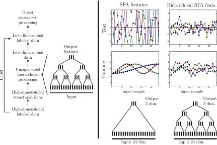
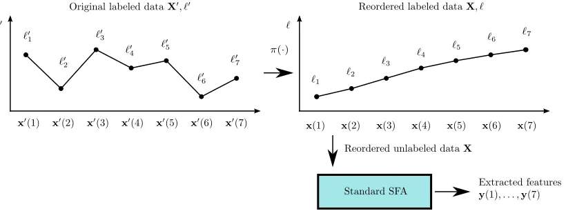
Given a large number of high-dimensional labeled data, supervised learning algorithms can often not be applied due to prohibitive computational requirements. In such cases we propose the following general scheme based on GSFA/SFA, illustrated in Figure 1 (left):
1. Transform the labeled data to structured data, where the label information is implicitly en-coded in the connections between the data points (samples). This permits using unsupervised learning algorithms, such as SFA, or its extension GSFA.
2. Use hierarchical processing to reduce the dimensionality, resulting in low-dimensional data with component similarities strongly dependent on the graph connectivity. Since the label information is encoded in the graph connectivity, the low-dimensional data are highly pre-dictive of the labels. Hierarchical processing (Section 2.4) is an efficient divide-and-conquer approach for high-dimensional data with SFA and GSFA.
4. Use standard supervised learning methods on the low-dimensional labeled data to estimate the labels. The unsupervised hierarchical network plus the supervised direct method together constitute the classifier or regression architecture.
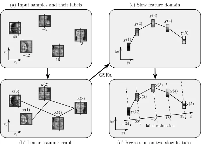
In the case of GSFA, the structured training data is called training graph, a weighted graph that has vertices representing the samples, node weights specifyinga priorisample probabilities, and edge weights indicating desired output similarities, as derived from the labels. Details are given in Section 3. This structure permits us to extend SFA to extract features from the data points that tend to reflect similarity relationships between their labels without the need to reproduce the labels themselves. A concrete example of the application of the method to a regression problem is illustrated in Figure 2. Various important advantages of GSFA are inherited from SFA:
• It allows hierarchical processing, which has various remarkable properties, as described in Section 2.4. One of them, illustrated in Figure 1 (right), is that the local application of SFA/GSFA to lower-dimensional data chunks typically results in less overfitting than non-hierarchical SFA/GSFA.
• SFA has a complexity of
O
(N)in the number of samplesNandO
(I3)in the number of dimen-sionsI(possibly after a nonlinear expansion). Hierarchical processing greatly reduces the lat-ter complexity down toO
(I). In practice, processing 100,000 samples of 10,000-dimensional input data can be done in less than three hours by using hierarchical SFA/GSFA without resorting to parallelization or GPU computing.• Typically no expensive parameter search is required. The SFA and GSFA algorithms them-selves are almost parameter free. Only the nonlinear expansion has to be defined. In hierar-chical SFA, the structure of the network has several parameters, but the choice is usually not critical.
In the next sections, we first recall the standard SFA optimization problem and algorithm. Then, we introduce the GSFA optimization problem, which incorporates the information contained in a training graph, and propose the GSFA algorithm, which solves this optimization problem. We recall how classification problems have been addressed with SFA and propose a training graph for doing this task with GSFA. Afterwards, we propose various graph structures for regression problems offering great computational efficiency and good accuracy. Thereafter, we experimentally evaluate and compare the performance of four training graphs to other common supervised methods (e.g., PCA+SVM) w.r.t. a particular regression problem closely related to face detection using real photographs. A discussion section concludes the article.
2. Standard SFA
In this section, we begin by introducing the slowness principle, which has inspired SFA. Afterwards, we recall the SFA optimization problem and the algorithm itself. We conclude the section with a brief introduction to hierarchical processing with SFA.
2.1 The Slowness Principle and SFA
Figure 1: (Left) Transformation of a supervised learning problem on high-dimensional data into a supervised learning problem on low-dimensional data by means of unsupervised hierar-chical processing on structured data, that is, without labels. This construction allows the solution of supervised learning problems on high-dimensional data when the dimension-ality and number of samples make the direct application of many conventional supervised algorithms infeasible. (Right) Example of how hierarchical SFA (HSFA) is more robust against overfitting than standard SFA. Useless data consisting of 25 random i.i.d. samples is processed by linear SFA and linear HSFA. Both algorithms reduce the dimensionality from 24 to 3 dimensions. Even though the training data is random, the direct applica-tion of SFA extracts the slowest features theoretically possible (optimal free responses), which is possible due to the number of dimensions and samples, permitting overfitting. However, it fails to provide consistent features for test data (e.g., standard deviations σtraining=1.0 vs. σtest=6.5), indicating lack of generalization. Several points even fall
outside the plotted area. In contrast, HSFA extracts much more consistent features (e.g., standard deviationsσtraining=1.0 vs. σtest=1.18) resulting in less overfitting.
Counter-intuitively, this result holds even though the HSFA network used has 7×6×3=126 free parameters, many more than the 24×3=72 free parameters of direct SFA.
Figure 2: Illustration of the application of GSFA to solve a regression problem. (a) The input sam-ples are 128×128-pixel images with labels indicating the horizontal position of the center of the face. (b) A training graph is constructed using the label information. In this ex-ample, only images with most similar labels are connected resulting in a linear graph. (c) The data dimensionality is reduced with GSFA, yielding in this case 3-dimensional feature vectors plotted in the first two dimensions. (d) The application of standard regres-sion methods to the slow features (e.g., linear regresregres-sion) generates the label estimates. In theory, the labels can be estimated fromy1 alone. In practice, performance is usually
improved by using not one, but a few slow features.
(Wiskott and Sejnowski, 2002; Franzius et al., 2011). Berkes and Wiskott (2005) subsequently used it for learning complex-cell receptive fields and Franzius et al. (2007) for place cells in the hippocampus. Recently, researchers have begun using SFA for various technical applications (see Escalante-B. and Wiskott, 2012, for a review).
2.2 Standard SFA Optimization Problem
The SFA optimization problem can be stated as follows (Wiskott, 1998; Wiskott and Sejnowski, 2002; Berkes and Wiskott, 2005). Given an I-dimensional input signalx(t) = (x1(t), . . . ,xI(t))T,
wheret∈R, find an instantaneous vectorial functiong:RI→RJ within a function space
F
, that is,g(x(t)) = (g1(x(t)), . . . ,gJ(x(t)))T, such that for each componentyj(t)def
=gj(x(t))of the output
signaly(t)def=g(x(t)), for 1≤ j≤J, the objective function ∆(yj)
def
=hy˙j(t)2it is minimal (delta value) (1)
under the constraints
hyj(t)it =0(zero mean), (2)
hyj(t)2it =1(unit variance), (3)
hyj(t)yj′(t)it =0,∀j′< j(decorrelation and order). (4)
The delta value∆(yj)is defined as the time average(h·it)of the squared derivative ofyj and is
therefore a measure of the slowness (or rather fastness) of the signal. The constraints (2–4) assure that the output signals are normalized, not constant, and represent different features of the input signal. The problem can be solved iteratively beginning withy1(the slowest feature extracted) and finishing with yJ (an algorithm is described in the next section). Due to constraint (4), the delta
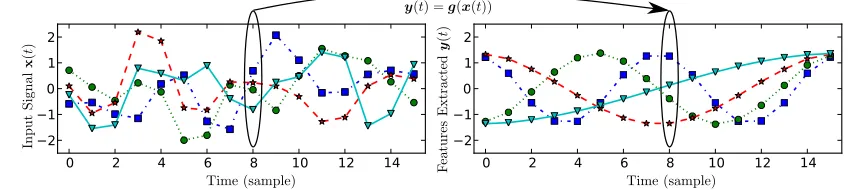
values are ordered, that is,∆(y1)≤∆(y2)≤ · · · ≤∆(yJ). See Figure 3 for an illustrative example.
0 2 4 6 8 10 12 14
2 1 0 1 2
Figure 3: Illustrative example of feature extraction from a 10-dimensional (discrete time) input signal. Four arbitrary components of the input (left) and the four slowest outputs (right) are shown. Notice that feature extraction is an instantaneous operation, even though the outputs are slow over time. This example was designed such that the features extracted are the slowest ones theoretically possible.
they result in overfitting. In extreme cases one obtains features such as those in Figure 3 (right) even when the hidden parameters of the input data lack such a precise structure. The problem is then evident when one extracts unstructured features from test data, see Figure 1 (right). An unrestricted function space is, however, useful for various theoretical analyses (e.g., Wiskott, 2003) because of its generality and mathematical convenience.
2.3 Standard Linear SFA Algorithm
The SFA algorithm is typically nonlinear. Even though kernelized versions have been proposed (Bray and Martinez, 2003; Vollgraf and Obermayer, 2006; B¨ohmer et al., 2012), it is usually im-plemented more directly with a nonlinear expansion of the input data followed by linear SFA in the expanded space. In this section, we recall the standard linear SFA algorithm (Wiskott and Se-jnowski, 2002), in which
F
is the space of all linear functions. Discrete time,t∈N, is used for the application of the algorithm to real data. Also the objective function and the constraints are adapted to discrete time. The input is then a single training signal (i.e., a sequence ofNsamples)x(t), where 1≤t≤N, and the time derivative ofx(t)is usually approximated by a sequence of differences of consecutive samples: ˙x(t)def≈x(t+1)−x(t), for 1≤t≤N−1.The output components take the formgj(x) =wTj(x−x¯), where ¯x def
= 1 N∑
N
t=1x(t)is the average
sample, which is subtracted, so that the output has zero-mean to conform with (2). Thus, in the linear case, the SFA problem reduces to finding an optimal set of weight vectors {wj}under the
constraints above, and it can be solved by linear algebra methods, see below. The covariance matrix is approximated by the sample covariance matrix
C= 1
N−1
N
∑
t=1(x(t)−x¯)(x(t)−x¯)T,
and the derivative second-moment matrixhx˙x˙Ti
t is approximated as
˙
C= 1
N−1
N−1
∑
t=1(x(t+1)−x(t))(x(t+1)−x(t))T.
Then, a sphered signal zdef= STx is computed, such that STCS=I for a sphering matrix S. Afterwards, theJ directions of least variance in the derivative signal˙z are found and represented by an I×J rotation matrix R, such that RTC˙zR=Λ, where C˙z
def
= h˙z˙zTit andΛ is a diagonal
matrix with diagonal elementsλ1≤λ2≤ · · · ≤λJ. Finally the algorithm returns the weight matrix W= (w1, . . . ,wJ), defined asW=SR, the features extractedy=WT(x−x¯), and∆(yj) =λj, for
1≤ j≤J. The linear SFA algorithm is guaranteed to find an optimal solution to the optimization problem (1–4) in the linear function space, for example, the first component extracted is the slowest possible linear feature. A more detailed description of the linear SFA algorithm is provided by Wiskott and Sejnowski (2002).
The complexity of the linear SFA algorithm described above is
O
(NI2+I3) where N is the number of samples andIis the input dimensionality (possibly after a nonlinear expansion), thus for high-dimensional data standard SFA is not feasible.1In practice, it has a speed comparable to PCA, even though SFA also takes into account the temporal structure of the data.1. The problem is still feasible ifNis small enough so that one might apply singular value decomposition methods.
2.4 Hierarchical SFA
To reduce the complexity of SFA, a divide-and-conquer strategy to extract slow features is usually effective (e.g., Franzius et al., 2011). For instance, one can spatially divide the data into lower-dimensional blocks of dimension I′ ≪I and extract J′ <I′ local slow features separately with different instances of SFA, the so-called SFA nodes. Then, one uses another SFA node in a next layer to extract global slow features from the local slow features. Since each SFA node performs dimensionality reduction, the input dimension of the top SFA node is much less thanI. This strategy can be repeated iteratively until the input dimensionality at each node is small enough, resulting in a multi-layer hierarchical network. Due to information loss before the top node, this does not guarantee optimal global slow features anymore. However it has shown to be effective in many practical experiments, in part because low-level features are spatially localized in most real data.
Interestingly, hierarchical processing can also be seen as a regularization method, as shown in Figure 1 (right), leading to better generalization. An additional advantage is that the nonlinearity accumulates across layers, so that even when using simple expansions the network as a whole can realize a complex nonlinearity (Escalante-B. and Wiskott, 2011).
3. Graph-Based SFA (GSFA)
In this section, we first present a generalized representation of the training data used by SFA called training graph. Afterwards, we propose the GSFA optimization problem, which is defined in terms of the nodes, edges and weights of such a graph. Then, we present the GSFA algorithm and a probabilistic model for the generation of training data, connecting SFA and GSFA.
3.1 Organization of the Training Samples in a Graph
Learning from a single (multi-dimensional) time series (i.e., a sequence of samples), as in standard SFA, is motivated from biology, because the input data is assumed to originate from sensory per-ception. In a more technical and supervised learning setting, the training data need not be a time series but may be a set of independent samples. However, one can use the labels to induce structure. For instance, face images may come from different persons and different sources but can still be ordered by, say, age. If one arranges these images in a sequence of increasing age, they would form a linear structure that could be used for training much like a regular time series.
The central contribution of this work is the consideration of a more complex structure for train-ing SFA called traintrain-ing graph. In the example above, one can then introduce a weighted edge between any pair of face images according to some similarity measure based on age (or other crite-ria such as gender, race, or mimic expression), with high similarity resulting in large edge weights. The original SFA objective then needs to be adapted such that samples connected by large edge weights yield similar output values.
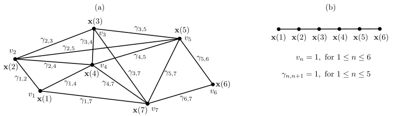
In mathematical terms, the training data is represented as a training graphG= (V,E)(illustrated in Figure 4) with a setVof verticesx(n)(each vertex/node being a sample), and a setEof edges
(x(n),x(n′)), which are pairs of samples, with 1≤n,n′≤N. The indexn(orn′) substitutes the time variablet. The edges are undirected and have symmetric weights
that indicate the similarity between the connected vertices; also each vertexx(n)has an associated weightvn>0, which can be used to reflect its importance, frequency, or reliability. For instance,
a sample occurring frequently in an observed phenomenon should have a larger weight than a rare sample. This representation includes the standard time series as a special case in which the graph has a linear structure and all node and edge weights are identical (Figure 4.b). How exactly edge weights are derived from label values will be elaborated later.
Figure 4: (a) Example of a training graph with N =7 vertices. (b) A regular sample sequence (time-series) represented as a linear graph suitable for GSFA.
3.2 GSFA Optimization Problem
We extend the concept of slowness, originally conceived for sequences of samples, to data structured in a training graph making use of its associated edge weights. The generalized optimization problem can then be formalized as follows. For 1≤ j≤J, find featuresyj(n), where 1≤n≤N, such that
the objective function
∆j def
= 1
R
∑
n,n′γn,n′(yj(n′)−yj(n))2is minimal (weighted delta value) (6)
under the constraints
1
Q
∑
n vnyj(n) =0(weighted zero mean), (7)1
Q
∑
n vn(yj(n))2=1(weighted unit variance),and (8)
1
Q
∑
n vnyj(n)yj′(n) =0,for j′<j(weighted decorrelation), (9)
with
Rdef=
∑
n,n′
γn,n′, (10)
Qdef=
∑
n
Compared to the original SFA problem, the vertex weights generalize the normalization con-straints, whereas the edge weights extend the objective function to penalize the difference between the outputs of arbitrary pairs of samples. Of course, the factor 1/Rin the objective function is not essential for the minimization problem. Likewise, the factor 1/Qcan be dropped from (7–9). These factors, however, provide invariance to the scale of the edge weights as well as to the scale of the node weights, and serve a normalization purpose.
By definition (see Section 3.1), training graphs are undirected and have symmetric edge weights. This does not cause any loss of generality and is justified by the GSFA optimization problem above. Its objective function (6) is insensitive to the direction of an edge because the sign of the output difference cancels out during the computation of∆j. It therefore makes no difference whether we
chooseγn,n′=2 andγn′,n=0 orγn,n′ =γn′,n=1, for instance. We note also thatγn,nmultiplies with zero in (6) and only enters into the calculation ofR. The variablesγn,nare kept only for mathematical
convenience.
3.3 Linear Graph-Based SFA Algorithm (Linear GSFA)
Similarly to the standard linear SFA algorithm, which solves the standard SFA problem in the lin-ear function space, here we propose an extension that computes an optimal solution to the GSFA problem within the same space. Let the verticesV={x(1), . . . ,x(N)}be the input samples with weights{v1, . . . ,vN}and the edgesEbe the set of edges(x(n),x(n′))with edge weightsγn,n′. To simplify notation we introduce zero edge weightsγn,n′=0 for non-existing edges(x(n),x(n′))∈/E. The linear GSFA algorithm differs from the standard version only in the computation of the matrices
CandC˙, which now take into account the neighbourhood structure (samples, edges, and weights) specified by the training graph.
The sample covariance matrixCGis defined as:
CG
def
= 1
Q
∑
n vn(x(n)−xˆ)(x(n)−xˆ) T = 1Q
∑
n vnx(n)(x(n))T−xˆxˆT, (12)
where
ˆ
x def= 1
Q
∑
n vnx(n) (13)is the weighted average of all samples. The derivative second-moment matrixC˙G is defined as:
˙ CG
def
= 1
Rn
∑
,n′γn,n′ x(n′)−x(n) x(n′)−x(n)T. (14)
Given these matrices, the computation of W is the same as in the standard algorithm (Sec-tion 2.3). Thus, a sphering matrixSand a rotation matrixRare computed with
STCGS= I, and (15)
RTSTC˙GSR= Λ, (16)
where Λis a diagonal matrix with diagonal elements λ1≤λ2 ≤ · · · ≤λJ. Finally the algorithm
returns∆(y1), . . . ,∆(yJ),Wandy(n), where
W =SR, and (17)
3.4 Correctness of the Graph-Based SFA Algorithm
We now prove that the GSFA algorithm indeed solves the optimization problem (6–9). This proof is similar to the optimality proof of the standard SFA algorithm (Wiskott and Sejnowski, 2002). For simplicity, assume thatCGandC˙Ghave full rank.
The weighted zero mean constraint (7) holds trivially for anyW, because
∑
nvny(n)
(18) =
∑
n
vnWT(x(n)−xˆ)
= WT
∑
nvnx(n)−
∑
n′vn′xˆ !
(13,11)
= WT(Qxˆ−Qxˆ) =0.
We also find
I = RTIR (sinceRis a rotation matrix),
(15)
= RT(STCGS)R,
(17)
= WTCGW,
(12) = WT 1
Q
∑
n vn(x(n)−xˆ)(x(n)−xˆ) TW,(18) = 1
Q
∑
n vny(n)(y(n)) T,which is equivalent to the normalization constraints (8) and (9). Now, let us consider the objective function
∆j
(6) = 1
Rn
∑
,n′γn,n′ yj(n′)−yj(n)2
(14)
= wTjC˙Gwj
(17)
= rTjSTC˙GSrj
(16) = λj,
whereR= (r1, . . . ,rJ). The algorithm finds a rotation matrixRsolving(16)and yielding
increas-ing λs. It can be seen (cf. Adali and Haykin, 2010, Section 4.2.3) that this Ralso achieves the minimization of∆j, for j=1, . . . ,J, hence, fulfilling (6).
3.5 Probabilistic Interpretation of Training Graphs
In this section, we give an intuition for the relationship between GSFA and standard SFA. Readers less interested in this theoretical excursion can safely skip it. This section is inspired in part by the Markov chain introduced by Klampfl and Maass (2010).
graph. Contrary to the graph introduced by Klampfl and Maass (2010), the formulation here is not restricted to classification, accounting for any training graph irrespective of its purpose, and there is one state per sample rather than one state per class. In order for the equivalence of GSFA and SFA to hold, the vertex weights ˜vn and edge weights ˜γn,n′ of the graph must fulfil the following
normalization restrictions:
∑
n˜
vn = 1, (19)
∑
n′˜
γn,n′/v˜n = 1 ∀n, (20)
(5)
⇐⇒
∑
n′ ˜
γn′,n/v˜n = 1 ∀n, (21)
∑
n,n′ ˜γn,n′(20=,19)1. (22)
Restrictions (19) and (22) can always be assumed without loss of generality, because they can be achieved by a constant scaling of the weights (i.e., ˜vn←v˜n/Q, ˜γn,n′←γ˜n,n′/R) without affecting the outputs generated by GSFA. Restriction (20) is fundamental because it limits the graph connectivity, and indicates (after multiplying with ˜vn) that each vertex weight should be equal to the sum of the
weights of all edges originating from such a vertex.
The Markov chain is then a sequenceZ1,Z2,Z3, . . . of random variables that can assume states that correspond to different input samples. Z1 is drawn from the initial distributionp1, which is
equal to the stationary distributionπ, where
πn = p1(n) def= Pr(Z1=x(n)) def= v˜n, (23)
and the transition probabilities are given by
Pnn′ def= Pr(Zt+1=x(n′)|Zt =x(n)) def= (1−ε)γ˜n,n′/v˜n+εv˜n′ =
limε→0 ˜
γn,n′/v˜n, (24)
(23)
=⇒ Pr(Zt+1=x(n′),Zt=x(n)) = (1−ε)˜γn,n′+εv˜nv˜n′ =
limε→0 ˜
γn,n′, (25)
(forZt stationary) with 0<ε≪1. Due to theε-term all states of the Markov chain can transition to
all other states including themselves, which makes the Markov chain irreducible and aperiodic, and therefore ergodic. Thus, the stationary distribution is unique and the Markov chain converges to it. The normalization restrictions (19), (20), and (22) ensure the normalization of (23), (24), and (25), respectively.
It is easy to see thatπ={v˜n}Nn=1is indeed a stationary distribution, since forpt(n) =v˜n pt+1(n) =Pr(Zt+1=x(n)) =
∑
n′
Pr(Zt+1=x(n)|Zt =x(n′))Pr(Zt=x(n′))
(23,24) =
∑
n′
((1−ε) (γ˜n′,n/v˜n′) +εv˜n)v˜n′
(21,19)
The time average of the input sequence is
µZ def
= hZtit
= hZiπ (since
M
is ergodic)(26) =
∑
n
˜
vnx(n)
(13)
= xˆ, (27)
and the covariance matrix is
C def= h(Zt−µZ)(Zt−µZ)Tit
(27)
= h(Z−xˆ)(Z−xˆ)Ti
π (since
M
is ergodic)(26) =
∑
n
˜
vn(x(n)−xˆ)(x(n)−xˆ)T
(12) = CG,
whereas the derivative covariance matrix is
˙
C def= hZ˙tZ˙Tt it
= hZ ˙˙ZTiπ (since
M
is ergodic)(25) =
∑
n,n′
((1−ε)˜γn,n′+εv˜nv˜n′) (x(n′)−x(n))(x(n′)−x(n))T, (28)
whereZt˙ def=Zt+1−Zt. Notice that limε→0C˙
(28)
= γ˜n,n′(x(n′)−x(n))(x(n′)−x(n))T
(14)
= C˙G.
There-fore, if a graph fulfils the normalization restrictions (19)–(22), GSFA yields the same features as standard SFA on the sequence generated by the Markov chain, in the limitε→0.
3.6 Construction of Training Graphs
One can, in principle, construct training graphs with arbitrary connections and weights. However, when the goal is to solve a supervised learning task, the graph created should implicitly integrate the label information. An appropriate structure of the training graphs depends on whether the goal is classification or regression. In the next sections, we describe each case separately. We have pre-viously implemented the proposed training graphs, and we have tested and verified their usefulness on real-world data (Escalante-B. and Wiskott, 2010; Mohamed and Mahdi, 2010; Stallkamp et al., 2011; Escalante-B. and Wiskott, 2012).
4. Classification with SFA
4.1 Clustered Training Graph
To generate features useful for classification, we propose the use of a clustered training graph
presented below (Figure 5). Assume there areSidentities/classes, and for each particular identity
s=1, . . . ,Sthere areNs samplesxs(n), wheren=1, . . . ,Ns, making a total ofN=∑sNssamples.
We define the clustered training graph as a graphG= (V,E)with verticesV={xs(n)}, and edges E={(xs(n),xs(n′))}fors=1, . . . ,S, andn,n′=1, . . . ,Ns. Thus all pairs of samples of the same
identity are connected, while samples of different identity are not connected. Node weights are identical and equal to one, that is,∀s,n: vs
n=1. In contrast, edge weights,γsn,n′ =1/Ns ∀n,n′,
depend on the cluster size.2 Otherwise identities with a largeN
swould be over-represented because
the number of edges in the complete subgraph for identitys grows quadratically with Ns. These
weights directly fulfil the normalization restriction (20). As usual, a trivial scaling of the node and edge weights suffices to fulfil restrictions (19) and (22), allowing the probabilistic interpretation of the graph. The optimization problem associated to this graph explicitly demands that samples from the same object identity should be typically mapped to similar outputs.
Figure 5: Illustration of aclusteredtraining graph used for a classification problem. All samples be-longing to the same object identity form fully connected subgraphs. Thus, forSidentities there areScomplete subgraphs. Self-loops not shown.
4.2 Efficient Learning Using the Clustered Training Graph
At first sight, the large number of edges, ∑sNs(Ns+1)/2, seems to introduce a computational
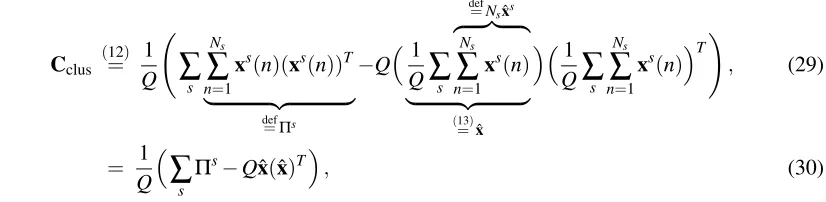
burden. Here we show that this is not the case if one exploits the symmetry of the clustered training graph. From (12), the sample covariance matrix of this graph using the node weights vsn =1 is (notice the definition ofΠsand ˆxs):
Cclus
(12) = 1
Q
∑
s Ns∑
n=1xs(n)(xs(n))T
| {z }
def
=Πs
−Q1 Q
∑
sdef
=Nsxˆs z }| {
Ns
∑
n=1xs(n)
| {z }
(13)
=xˆ
1
Q
∑
s Ns∑
n=1xs(n)T
!
, (29)
= 1
Q
∑
sΠs−Qxˆ(xˆ)T, (30)
whereQ(11=)∑s∑nN=s11=∑sNs=N.
From (14), the derivative covariance matrix of the clustered training graph using edge weights γs
n,n′ =1/Nsis:
˙ Cclus
(14) = 1
R
∑
s1
Ns Ns
∑
n,n′=1(xs(n′)−xs(n))(xs(n′)−xs(n))T, (31)
= 1
R
∑
s1
Ns Ns
∑
n,n′=1
xs(n′)(xs(n′))T+xs(n)(xs(n))T−xs(n′)(xs(n))T−xs(n)(xs(n′))T,
(29) = 1
R
∑
s1
Ns Ns
Ns
∑
n=1xs(n)(xs(n))T+Ns Ns
∑
n′=1xs(n′)(xs(n′))T−2Nsxˆs(Nsxˆs)T !
,
(29) = 2
R
∑
s Π s−Nsxˆs(xˆs)T
, (32)
whereR(10=)∑s∑n,n′γsn,n′ =∑s∑n,n′1/Ns=∑s(Ns)2/Ns=∑sNs=N.
The complexity of computing Cclus using (29) or (30) is the same, namely
O
(∑sNs)(vector)operations. However, the complexity of computingC˙clus can be reduced from
O
(∑sNs2)operationsdirectly using (31) to
O
(∑sNs) operations using (32). This algebraic simplification allows us tocompute C˙clus with a complexity linear in N (and Ns), which constitutes an important speedup
since, depending on the application,Nsmight be larger than 100 and sometimes evenNs>1000.
Interestingly, one can show that the features learned by GSFA on this graph are equivalent to those learned by FDA (see Section 7).
4.3 Supervised Step for Classification Problems
Consistent with FDA, the theory of SFA using an unrestricted function space (optimal free re-sponses) predicts that, for this type of problem, the firstS−1 slow features extracted are orthogonal step functions, and are piece-wise constant for samples from the same identity (Berkes, 2005a). This closely approximates what has been observed empirically, which can be informally described as features that are approximately constant for samples of the same identity, with moderate noise.
When the features extracted are close to the theoretical predictions (e.g., their ∆-values are small), their structure is simple enough that one can use even a modest supervised step after SFA, such as a nearest centroid or a Gaussian classifier (in which a Gaussian distribution is fitted to each class) onS−1 slow features or less. We suggest the use of a Gaussian classifier because in practice we have obtained better robustness when enough training data is available. While a more powerful classification method, such as an SVM, might also be used, we have found only a small increase in performance at the cost of longer training times.
5. Regression with SFA
Regression problems can be address with SFA through multiple methods. The fundamental idea is to treat labels as the value of a hidden slow parameter that we want to learn. In general, SFA will not extract the label values exactly. However, optimization for slowness implies that samples with similar label values are typically mapped to similar output values. After SFA reduces the dimensionality of the data, a complementary explicit regression step on a few features solves the original regression problem.
In this section, we propose four SFA-based methods that explicitly use available labels. The first method is calledsample reorderingand employs standard SFA, whereas the remaining ones employ GSFA with three different training graphs calledsliding window,serial, andmixed (Sections 5.1– 5.4). The selection of the explicit regression step for post-processing is discussed in Section 5.5.
5.1 Sample Reordering
LetX′= (x′(1), . . . ,x′(N))be a sequence ofN data samples with labelsℓ′= (ℓ′1, . . . , ℓ′N). The data is reordered by means of a permutationπ(·)in such a way that the labels become monotonically increasing. The reordered samples areX= (x(1), . . . ,x(N)), wherex(n) =x′(π(n)), and their labels areℓ= (ℓ1, . . . , ℓN)withℓl≤ℓl+1. Afterwards the sequenceXis used to train standard SFA using
the regular single-sequence method (Figure 6).
Figure 6: Sample reordering approach. Standard SFA is trained with a reordered sample sequence, in which the hidden labels are increasing.
Since the ordered label values only increase, they change very slowly and should be found by SFA (or actually some increasing/decreasing function of the labels that also fulfils the normalization conditions). Clearly, SFA could only extract this information if the samples indeed intrinsically contain information about the labels such that it is possible to extract the labels from them. Due to limitations of the feature space considered, insufficient data, noise, etc., one typically obtains noisy and distorted versions of the predicted signals.
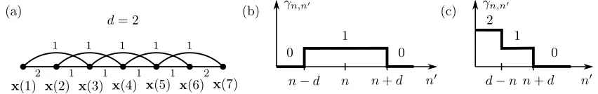
5.2 Sliding Window Training Graph
This is an improvement over the method above in which GSFA facilitates the consideration of more connections. Starting from the reordered sequence Xas defined above, a training graph is constructed, in which each sample x(n) is connected to its d closest samples to the left and to the right in the order given byX. Thus, x(n) is connected to the samplesx(n−d), . . . ,x(n−1),
x(n+1), . . . ,x(n+d) (Figure 7.a). In this graph, the vertex weights are constant, that is,vn=1,
and the edge weights typically depend on the distance of the samples involved, that is,∀n,n′: γ n,n′=
f(|n′−n|), for some function f(·)that specifies the shape of a “weight window”. The simplest case is a square weight window defined by γn,n′ =1 if |n′−n| ≤d andγn,n′ =0 otherwise. For the experiments in this article, we employ amirroredsliding window with edge weights
γn,n′ =
2, if n+n′≤d+1 orn+n′≥2N−1,
1, if |n′−n| ≤d,n+n′>d+1 andn+n′<2N−1,
0, otherwise.
These weights compensate the limited connectivity of the few first and last samples (which are connected byd to 2d−1 edges) in contrast to intermediate samples (connected by 2dedges). Pre-liminary experiments suggest that such compensation slightly improves the quality of the extracted features, as explained below.
Figure 7: (a) A mirrored square sliding window training graph with a half-width ofd=2. Each vertex is thus adjacent to at most 4 other vertices. (b) Illustration of the edge weights of an intermediate nodex(n)for an arbitrary window half-widthd. (c) Edge weights for a nodex(n) close to the left extreme (n<d). Notice that the sum of the edge weights is also approximately 2dfor extreme nodes.
The occurrence of pathological solutions depends on the concrete data samples, feature space, and training graph. A necessary condition is that the graph is connected because, as discussed in Section 4, for disconnected graphs GSFA has a strong tendency to produce a representation suitable for classification rather than regression. After various experiments, we have found useful to enforce the normalization restriction (20) at least approximately (after node and edge weights have been normalized). This ensures that the samples are connected sufficiently strongly to the other ones, relative to their own node weight. Of course, one should not resort to self-loopsγn,n6=0 to trivially
fulfil the restriction.
The improved continuity of the features appears to also benefit performance after the supervised step. This is the reason why we make the node weights of the first and last groups of samples in the serial training graph weaker, the intra-group connections of the first and last groups of samples in the mixed graph stronger, and introduced mirroring for the square sliding window graph.
In the sliding window training graph with arbitrary window, the computation of CG andC˙G
requires
O
(dN) operations. If the window is square (mirrored or not), the computation can be improved toO
(N)operations by using accumulators for sums and products and reusing intermediate results. While largerd implies more connections, connecting too distant samples is undesired. The selection ofdis non-crucial and done empirically.5.3 Serial Training Graph
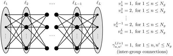
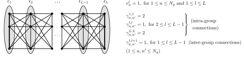
Theserialtraining graph is similar to the clustered training graph used for classification in terms of construction and efficiency. It results from discretizing the original labelsℓinto a relatively small set of discrete labels of sizeL, namely{ℓ1, . . . , ℓL}, whereℓ1< ℓ2<· · ·< ℓL. As described below,
faster training is achieved ifLis small, for example, 3≤L≪N.
In this graph, the vertices are grouped according to their discrete labels. Every sample in the group with labelℓl is connected to every sample in the groups with labelℓl+1andℓl−1 (except the
samples in the first and last groups, which can only be connected to one neighbouring group). The only existing connections are inter-group connections, no intra-group connections are present.
The samples used for training are denoted byxl(n), where the indexl(1≤l≤L) denotes the
group (discrete label) andn(1≤n≤Nl) denotes the sample within such a group. For simplicity,
we assume here that all groups have the same numberNgof samples: ∀l: Nl =Ng. Thus the total
number of samples is N=LNg. The vertex weight of xl(n) is denoted by vln, where vln =1 for l∈ {1,L}andvln=2 for 1<l<L. The edge weight of the edge(xl(n),xl+1(n′))is denoted by γln,,ln+′1, and we use the same edge weight for all connections: ∀n,n′,l: γln,,ln+′1=1. Thus, all edges have a weight of 1, and all samples are assigned a weight of 2 except for the samples in the first and last groups, which have a weight of 1 (Figure 8). The reason for the different weights in the first and last groups is to improve feature quality by enforcing the normalization restriction (20) (after node and edge weight normalization). Notice that since any two vertices of the same group are adjacent to exactly the same neighbours, they are likely to be mapped to similar outputs by GSFA.
The sum of vertex weights is Q(11=)Ng+2Ng(L−2) +Ng=2Ng(L−1) and the sum of edge
weights isR(10= () L−1)(Ng)2, which is also the number of connections considered. Unsurprisingly,
the structure of the graph can be exploited to train GSFA efficiently. Similarly to the clustered training graph, define the average of the samples from the grouplas ˆxldef=∑nxl(n)/Ng, the sum of
the products of samples from groupl asΠl =∑
Figure 8: Illustration of a serial training graph with L discrete labels. Even though the original labels of two samples might differ, they will be grouped together if they have the same discrete label. In the figure, a bigger node represents a sample with a larger weight, and the ovals represent the groups.
as:
ˆ
x def= 1
Q
∑
n x1(n) +xL(n) +2L
∑
−1 l=2xl(n)
!
= 1
2(L−1) xˆ
1+xˆL+2L
∑
−1 l=2ˆ
xl !
. (33)
From (12), the sample covariance matrix accounting for the weights vln of the serial training graph is:
Cser
(12,33) = 1
Q
∑
n x1(n)(x1(n))T+2L−1
∑
l=2∑
nxl(n)(xl(n))T+
∑
n
xL(n)(xL(n))T−Qxˆ(xˆ)T
!
= 1
Q Π
1+ΠL+2L−1
∑
l=2Πl−Qxˆ′(xˆ′)T
!
.
From (14), the matrixC˙Gusing the edgesγln,,ln+′1defined above is:
˙ Cser
(14) = 1
R L−1
∑
l=1n∑
,n′(xl+1(n′)−xl(n))(xl+1(n′)−xl(n))T (34)
= 1
R L−1
∑
l=1n∑
,n′
xl+1(n′)(xl+1(n′))T+xl(n)(xl(n))T−xl(n)(xl+1(n′))T−xl+1(n′)(xl(n))T
= 1
R L−1
∑
l=1
∑
n′Πl+1+Πl−
∑
n
xl(n)
∑
n′
xl+1(n′)T−
∑
n′
xl+1(n′)
∑
n
xl(n)T
=Ng
R L−1
∑
l=1
Πl+1+Πl−Ngxˆl(xˆl+1)T−Ngxˆl+1(xˆl)T
. (35)
By using (35) instead of (34), the slowest step in the computation of the covariance matrices, which is the computation of C˙ser, can be reduced in complexity from
O
(L(Ng)2) to onlyO
(N)operations (N=LNg), which is of the same order as the computation ofCser. Thus, for the same
Discretization introduces some type of quantization error. While a large number of discrete labelsLresults in a smaller quantization error, having too many of them is undesired because fewer edges would be considered, which would increase the number of samples needed to reduce the overall error. For example, in the extreme case ofNg=1 andL=N, this method does not bring any
benefit because it is almost equivalent to the sample reordering approach (differing only due to the smaller weights of the first and last samples).
5.4 Mixed Training Graph
The serial training graph does not have intra-group connections, and therefore the output differences of samples with the same label are not explicitly being minimized. One argument against intra-group connections is that if two vertices are adjacent to the same set of vertices, their corresponding samples are already likely to be mapped to similar outputs. However, in some cases, particularly for small numbers of training samples, additional intra-group connections might indeed improve robustness. We thus conceived themixedtraining graph (Figure 9), which is a combination of the serial and clustered training graph and fulfils the consistency restriction (20). In the mixed training graph, all nodes and edges have a weight of 1, except for the intra-group edges in the first and last groups, which have a weight of 2. As expected, the computation of the covariance matrices can also be done efficiently for this training graph (details omitted).
Figure 9: Illustration of the mixed training graph. Samples having the same label are fully con-nected (intra-group connections, represented with vertical edges) and all samples of ad-jacent groups are connected (inter-group connections). All vertex and edge weights are equal to 1 except for the intra-group edge weights of the first and last groups, which are equal to 2 as represented by thick lines.
5.5 Supervised Step for Regression Problems
There are at least three approaches to implement the supervised step on top of SFA to learn a mapping from slow features to the labels. The first one is to use a method such as linear or nonlinear regression. The second one is to discretize the original labels to a small discrete set{ℓ˜1, . . . ,ℓ˜˜
L}
that the input samplexwith slow featuresy=g(x)belongs to the group with (discretized) label ˜ℓl.
Class probabilities can be used to provide a more robust estimation of a soft (continuous) labelℓ, better suited to the particular loss function. For instance, one can use
ℓ def=
˜ L
∑
l=1˜
ℓl·P(Cℓ˜l|y) (36)
if the loss function is the RMSE, where the slow featuresymight be extracted using any of the four SFA-based methods for regression above. Other loss functions, such as the Mean Average Error (MAE), can be addressed in a similar way.
We have tested these three approaches in combination with supervised algorithms such as lin-ear regression, and classifiers such as nlin-earest neighbour, nlin-earest centroid, Gaussian classifier, and SVMs. We recommend using the soft labels computed from the class probabilities estimated by a Gaussian classifier because in most of our experiments this method has provided best performance and robustness. Of course, other classifiers providing class probabilities could also be used.
6. Experimental Evaluation of the Methods Proposed
In this section, we evaluate the performance of the supervised learning methods based on SFA pre-sented above. We consider two concrete image analysis problems using real photograph databases, the first one for classification and the second one for regression.
6.1 Classification
For classification, we have proposed the clustered training graph. As mentioned in Section 4.2, when this graph is used, the outputs of GSFA are equivalent to those of FDA. Since FDA has been used and evaluated exhaustively, here we only verify that our implementation of GSFA generates the expected results when trained with such a graph.
The German Traffic Sign Recognition Benchmark (Stallkamp et al., 2011) was chosen for the experimental test. This was a competition with the goal of classifying photographs of 43 different traffic signs taken on German roads under uncontrolled conditions with variations in lighting, sign size, and distance. No detection step was necessary because the true position of the signs was included as annotations, making this a pure classification task and ideal for our test. We participated in the online version of the competition, where 26,640 labeled images were provided for training and 12,569 images without label for evaluation (classification rate was computed by the organisers, who had ground-truth data).
Two-layer nonlinear cascaded (non-hierarchical) SFA was employed. To achieve good perfor-mance, the choice of the nonlinear expansion function is crucial. If it is too simple (e.g., low-dimensional), it does not solve the problem; if it is too complex (e.g., high-low-dimensional), it might overfit to the training data and not generalize well to test data. In all the experiments done here, a compact expansion that only doubles the data dimension was employed,xT 7→xT,(|x|0.8)T, where
Our method, complemented by a Gaussian classifier on 42 slow features, achieved a recognition rate of 96.4% on test data.3 This, as expected, was similar to the reported performance of various methods based on FDA participating in the same competition. For comparison, human performance was 98.81%, and a convolutional neural network gave top performance with a 98.98% recognition rate.
6.2 Regression
The remaining training graphs have all been designed for regression problems and were evaluated with the problem of estimating the horizontal position of a face in frontal face photographs, an important regression problem because it can be used as a component of a face detection system, as we proposed previously (see Mohamed and Mahdi, 2010). In our system, face detection is decomposed into the problems of the estimation of the horizontal position of a face, its vertical position, and its size. Afterwards, face detection is refined by locating each eye more accurately with the same approach applied now to the eyes instead of to the face centers. Below, we explain this regression problem, the algorithms evaluated, and the results in more detail.
6.2.1 PROBLEM ANDDATASETDESCRIPTION
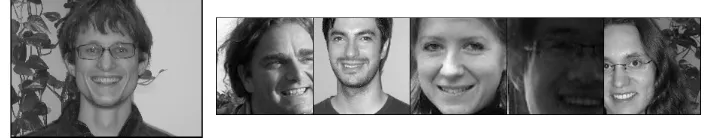
To increase image variability and improve generalization, face images from several databases were used, namely 1,521 images from BioID (Jesorsky et al., 2001), 9,030 from CAS-PEAL (Gao et al., 2008), 5,479 from Caltech (Fink et al.), 9,113 from FaceTracer (Kumar et al., 2008), and 39,328 from FRGC (Phillips et al., 2005) making a total of 64,471 images, which were automatically pre-processed through a pose-normalization and a pose-reintroduction step. In the first step, each image was converted to greyscale and pose-normalized using annotated facial points so that the face is cen-tered,4has a fixed eye-mouth-triangle area, and the resulting pose-normalized image has a resolution of 256×192 pixels. In the second step, horizontal and vertical displacements were re-introduced, as well as scalings, so that the center of the face deviates horizontally at most±45 pixels from the center of the image. The vertical position and the size of the face were randomized, so that ver-tically the face center deviates at most±20 pixels, and the smallest faces are half the size of the largest faces (a ratio of at most 1 to 4 in area). Interpolation (e.g., needed for scaling and sub-pixel displacements) was done using bicubic interpolation. At last, the images were cropped to 128×128 pixels.
Given a pre-processed input image, as described above, with a face at position(x,y)w.r.t. the image center and sizez, the regression problem is then to estimate thex-coordinate of the center of the face. The range of the variablesx,yand zis bounded to a box, so that one does not have to consider extremely small faces, for example. To assure a robust estimation for new images, invariance to a large number of factors is needed, including the vertical position of the face, its size, the expression and identity of the subject, his or her accessories, clothing, hair style, the lighting conditions, and the background.
3. Interestingly, GSFA did not provide best performance directly on the pixel data, but on precomputed HOG features. Ideally, pre-processing is not needed if SFA has an unrestricted feature space. In practice, knowing a good low-dimensional set of features for the particular data is beneficial. Applying SFA to such features, as commonly done with other machine learning algorithms, can reduce overfitting.
4. The center of a face was defined here as14LE+1 4RE+
1
2M, whereLE,REandMare the coordinates of the centers
Figure 10: Example of a pose-normalized image (left), and various images after pose was reintro-duced illustrating the final range of vertical and horizontal displacements, as well as the face sizes (right).
The pose-normalized images were randomly split in three data sets of 30,000, 20,000 and 9,000 images. The first data set was used to train the dimensionality reduction method, the second one to train the supervised post-processing step, and the last one for testing. To further exploit the images available, the pose-normalized images of each data set were duplicated, resulting in two pose-reintroduced images per input image, that is, a single input image exclusively belongs to one of the three data sets, appearing twice in it with two different poses. Hence, the final size of the data sets is 60,000, 40,000 and 18,000 pre-processed images, respectively.
6.2.2 DIMENSIONALITY-REDUCTIONMETHODSEVALUATED
The resolution of the images and their number make it less practical to directly apply SFA and the majority of supervised methods, such as an SVM, and unsupervised methods, such as PCA/ICA/LLE, to the raw images. We circumvent this by using three efficient dimensionality reduction methods, and by applying supervised processing on the lower-dimensional features extracted. The first two methods are efficient hierarchical implementations of SFA and GSFA (referred to as HSFA without distinction). The nodes in the HSFA networks first expand the data using the 0.8Expexpansion function (see Section 6.1) and then apply SFA/GSFA to it, except for the nodes in the first layer in which additionally PCA is applied before the expansion preserving 13 out of 16 principal compo-nents. For comparison, we use a third method, a hierarchical implementation of PCA (HPCA), in which all nodes do pure PCA. The structure of the hierarchies for the HSFA and PCA networks is described in Table 1. In contrast to other works (e.g., Franzius et al., 2007), weight-sharing was not used at all, improving feature specificity at the lowest layers. The input to the nodes (fan-in) comes mostly from two nodes in the previous layer. This small fan-in reduces the computational cost be-cause the input dimensionality is minimized. This also results in networks with a large number of layers potentiating the accumulation of non-linearity across the network. Non-overlapping receptive fields were used because in previous experiments with similar data they showed good performance at a smaller computational cost.
The following dimensionality-reduction methods were evaluated (one based on SFA, four based on GSFA, and one based on PCA).
• SFA using sample reordering (reordering).
Layer size node output dim. output dim.
fan-in per HSFA node per HPCA node
0 (input image) 128×128 pixels — — —
1 32×32 nodes 4×4 13 13
2 16×32 nodes 2×1 20 20
3 16×16 nodes 1×2 35 35
4 8×16 nodes 2×1 60 60
5 8×8 nodes 1×2 60 100
6 4×8 nodes 2×1 60 120
7 4×4 nodes 1×2 60 120
8 2×4 nodes 2×1 60 120
9 2×2 nodes 1×2 60 120
10 1×2 nodes 2×1 60 120
11 (top node) 1×1 nodes 1×2 60 120
Table 1: Structure of the SFA and PCA deep hierarchical networks. The networks only differ in the type of processing done by each node and in the number of features preserved. For HSFA an upper bound of 60 features was set, whereas for HPCA at most 120 features were preserved. A node with a fan-in ofa×bis driven by a rectangular array of nodes (or pixels for the first layer) with such a shape, located in the preceding layer.
• GSFA with a mirrored sliding window graph withd=64 (MSW64).
• GSFA with a serial training graph withL=50 groups ofNg=600 images (serial).
• GSFA with a mixed graph and the same number of groups and images (mixed).
• A hierarchical implementation of PCA (HPCA).
It is impossible to compare GSFA against all the dimensionality reduction and supervised learn-ing algorithms available, and therefore we made a small selection thereof. We chose HPCA for efficiency reasons and because it is likely to be a good dimensionality reduction algorithm for the problem at hand since principal components code well the coarse structure of the image including the silhouette of the subjects, allowing for a good estimation of the position of the face. Thus, we believe that HPCA (combined with various supervised algorithms) is a fair point of comparison, and a good representative among generic machine learning algorithms for this problem. For the data employed, 120 HPCA features at the top node explain 88% of the data variance, suggesting that HPCA is indeed a good approximation to PCA in this case.
The evolution across the hierarchical network of the two slowest features extracted by HSFA is illustrated in Figure 11.
6.2.3 SUPERVISED POST-PROCESSINGALGORITHMSCONSIDERED
Figure 11: Evolution of the slow features extracted from test data after layers 1, 4, 7 and 11 of a GSFA network trained with the serial training graph. A central node was selected from each layer, and three plots are provided, that is,y2vsy1,nvsy1, andy2vsn. Hierarchical processing results in progressively slower features as one moves from the first to the top layer. The solid line in the plots of the top node represents the optimal free responses, which are the slowest possible features one can obtain using an unrestricted mapping, as predicted theoretically (Wiskott, 2003). Notice how the features evolve from being mostly unstructured in the first layer to being similar to the free responses at the top node, indicating success at finding the hidden parameter changing most slowly for these data (i.e., the horizontal position of the faces).
• A nearest centroid classifier (NCC).
• Labels estimated using (36) and the class membership probabilities given by a Gaussian clas-sifier (Soft GC).
• A multi-class (one-versus-one) SVM (Chang and Lin, 2011) with a Gaussian radial basis kernel, and grid search for model selection.