Semi-Supervised Learning with Measure Propagation

Semi-Supervised Learning with Measure Propagation

Amarnag Subramanya [email protected]

Jeff Bilmes [email protected]

Department of Electrical Engineering University of Washington

Seattle, WA 98195, USA

Editor: Yoshua Bengio

Abstract

We describe a new objective for graph-based semi-supervised learning based on minimizing the Kullback-Leibler divergence between discrete probability measures that encode class membership probabilities. We show how the proposed objective can be efficiently optimized using alternating minimization. We prove that the alternating minimization procedure converges to the correct op-timum and derive a simple test for convergence. In addition, we show how this approach can be scaled to solve the semi-supervised learning problem on very large data sets, for example, in one instance we use a data set with over 108 samples. In this context, we propose a graph node or-dering algorithm that is also applicable to other graph-based semi-supervised learning approaches. We compare the proposed approach against other standard semi-supervised learning algorithms on the semi-supervised learning benchmark data sets (Chapelle et al., 2007), and other real-world tasks such as text classification on Reuters and WebKB, speech phone classification on TIMIT and Switchboard, and linguistic dialog-act tagging on Dihana and Switchboard. In each case, the proposed approach outperforms the state-of-the-art. Lastly, we show that our objective can be gen-eralized into a form that includes the standard squared-error loss, and we prove a geometric rate of convergence in that case.

Keywords: graph-based semi-supervised learning, transductive inference, large-scale semi-supervised

learning, non-parametric models

1. Introduction

In many applications, annotating training data is time-consuming, costly, tedious, and error-prone. For example, training an accurate speech recognizer requires large amounts of well annotated speech data (Evermann et al., 2005). In the case of document classification for Internet search, it is not feasible to accurately annotate sufficient number of web-pages for all categories of interest. The process of training classifiers with small amounts of labeled data and relatively large amounts of unlabeled data is known as semi-supervised learning (SSL). SSL lends itself as a useful technique in many machine learning applications as one only needs to annotate small amounts of data for training models.

is also related to the problem of transductive learning (Vladimir, 1998). In general, a learner is transductive if it is designed only for a closed data set, where the test set is revealed at training time. In practice, however, transductive learners can be modified to handle unseen data (Sindhwani et al., 2005; Zhu, 2005b). Chapelle et al. (2007, Chapter 25) gives a nice discussion on the relationship between SSL and transductive learning.

Graph-based SSL algorithms are an important sub-class of SSL techniques that have received much attention in the recent past (Zhu, 2005b; Chapelle et al., 2007). Here one assumes that the data (both labeled and unlabeled) is embedded within a low-dimensional manifold that may be rea-sonably expressed by a graph. Each data sample is represented by a vertex in a weighted graph with the weights providing a measure of similarity between vertices. Most graph-based SSL algorithms fall under one of two categories – those that use the graph structure to spread labels from labeled to unlabeled samples (Szummer and Jaakkola, 2001; Zhu and Ghahramani, 2002a) and those that op-timize a loss function based on smoothness constraints derived from the graph (Blum and Chawla, 2001; Zhu et al., 2003; Joachims, 2003; Belkin et al., 2005; Corduneanu and Jaakkola, 2003; Tsuda, 2005). In some cases, for example, label propagation (Zhu and Ghahramani, 2002a) and the har-monic functions algorithm (Zhu et al., 2003; Bengio et al., 2007), it can be shown that the two categories optimize a similar loss function (Zhu, 2005a; Bengio et al., 2007).

A large number of graph-based SSL algorithms attempt to minimize a loss function that is inherently based on squared-loss (Zhu et al., 2003; Bengio et al., 2007; Joachims, 2003). While squared-loss is optimal under a Gaussian noise model, it is not optimal in the case of classification problems. Another potential drawback in the case of some graph-based SSL algorithms (Blum and Chawla, 2001; Joachims, 2003) is that they assume binary classification tasks and thus require the use of sub-optimal (and often computationally expensive) approaches such as one vs. rest to solve multi-class problems. While it is often argued that the use of binary classifiers within a one vs. rest framework performs as well as true multi-class solutions (Rifkin and Klautau, 2004), our results on SSL problems suggest otherwise (see Section 7.2.2).

Further, there is a lack of principled approaches to incorporate label priors in graph-based SSL algorithms. Approaches such as class mass normalization (CMN) and label bidding are used as a post-processing step rather than being tightly integrated with the inference (Zhu and Ghahramani, 2002a). In this context, it is important to distinguish label priors from balance priors. Balance priors are used in some algorithms such as Joachims (2003) and discourage the scenario where all the unlabeled samples are classified as belonging to a single class (i.e., a degenerate solution). Balance priors impose selective pressure collectively on the entire set of resulting answers. Label priors, on the other hand, select the more desirable configuration for each answer individually without caring about properties of the overall set of resulting answers. In addition, many SSL algorithms, such as Joachims (2003) and Belkin et al. (2005), are unable to handle label uncertainty, where there may be insufficient evidence to justify only a single label for a labeled sample.

solved to date had about 900,000 samples (includes both labeled and unlabeled data) (Tsang and Kwok, 2006). Clearly, this is a fraction of the amount of unlabeled data at our disposal. For exam-ple, on the Internet alone, we create 1.6 billion blog posts, 60 billion emails, 2 million photos and 200,000 videos every day (Tomkins, 2008). In general, graph-based SSL algorithms that use matrix inversion (Zhu et al., 2003; Belkin et al., 2005) or eigen-based matrix decomposition (Joachims, 2003) do not scale very easily.

In Subramanya and Bilmes (2008), we proposed a new framework for graph-based SSL that in-volves optimizing a loss function based on Kullback-Leibler divergence (KLD) between probability measures defined for each graph vertex. These probability measures encode the class membership probabilities. The advantages of this new convex objective are: (a) it is naturally amenable to multi-class (>2) problems; (b) it can handle label uncertainty; and (c) it can integrate priors. Furthermore, the use of probability measures allows the exploitation of other well-defined functions of measures, such as entropy, to improve system performance. Subramanya and Bilmes (2008) also showed how the proposed objective can be optimized using alternating minimization (AM) (Csiszar and Tus-nady, 1984) leading to simple update equations. This new approach to graph-based SSL was shown to outperform other state-of-the-art SSL algorithms for the document and web page classification tasks. In this paper we extend the above work along the following lines –

1. We prove that AM on the proposed convex objective for graph-based SSL converges to the global optima. In addition we derive a test for convergence that does not require the compu-tation of the objective.

2. We compare the performance of the proposed approach against other state-of-the-art SSL approaches, such as manifold regularization (Belkin et al., 2005), label propagation (Zhu and Ghahramani, 2002a), and spectral graph transduction (Joachims, 2003) on a variety of tasks ranging from synthetic data sets to SSL benchmark data sets (Chapelle et al., 2007) to real-world problems such as phone classification, text classification, web-page classification and dialog-act tagging.

3. We propose a graph node ordering algorithm that is cache cognizant and makes obtaining a linear speedup with a parallel symmetric multi-processor (SMP) implementation more likely. As a result, the algorithms are able to scale to very large data sets. The node ordering al-gorithm is quite general and can be applied to graph-based SSL alal-gorithms such as Zhu and Ghahramani (2002a); Zhu et al. (2003). In one instance, we solve a SSL problem over a graph with 120 million vertices (which is quite a bit more than the previous largest size of 900,000 vertices). A useful byproduct of this experiment is the semi-supervised switchboard

transcription project (S3TP) which consists of phone level annotations of the Switchboard-I corpus generated in a semi-supervised manner (see Section 8.1, Subramanya and Bilmes,

2009).

5. A specific case of the Bregman divergence form is the standard squared-loss based objective, and we prove a geometric rate of convergence in this case in Appendix F

6. We discuss a principled approach to integrating label priors into the proposed objective (see Section 9.2).

7. We also show how our proposed objective can be extended to directed graphs (see Sec-tion 9.3).

2. Graph Construction

Let

D

l ={(xi,ri)}_i=1l be the set of labeled samples,

D

u={xi}l+u_i=l+1 the set of unlabeled samples

and

D

,_{

_D

_l,

_D

_{u}. Here riis an encoding of the labeled data and will be explained shortly. We are}

interested in solving the transductive learning problem, that is, given

D

, the task is to predict the labels of the samples in

D

u (for inductive see Section 7.4). We are given an undirected weighted

graph

G

= (V,E), where the vertices (nodes) V={1, . . . ,m}(m,l+u) are the data points in

D

and the edges E⊆V×V . Let V =Vl∪Vuwhere Vl is the set of labeled vertices and Vu the set of

unlabeled vertices.

G

may be represented via a matrix W referred to as the weight or affinity matrix. There are many ways of constructing the graph. In some applications, it might be a natural result of relationship between the samples in

D

, for example, consider the case where each vertex represents a web-page and the edges represent the links between web-pages. In other cases, such as the work of Fei and Changshui (2006), the graph is generated by performing an operation similar to local linear embedding (LLE) but constraining the LLE weights to be non-negative. In a majority of the applications, including those considered in this paper, we use k-nearest neighbor (NN) graphs. In our case here, we make use of symmetric k-NN graphs and so the edge weight wi j = [W]_{i j} is

given by

wi j= (

sim(xi,xj) if j∈

K

(i)or i∈

K

(j)

0 otherwise

where

K

(i) is the set of k-NN of xi (|

K

(i)|=k, ∀i) and sim(xi,xj) is a measure of similarity

between xiand xj(which are represented by nodes i and j). It is assumed that the similarity measure

is symmetric, that is, sim(x,y) =sim(y,x). Further sim(x,y)≥0. Some popular similarity measures include

sim(xi,xj) =e−

k_xi−_{x j}k2₂

2σ _{or sim(xi,xj) =cos(xi,xj) =} hxi,xji kxik2kxjk2

where kxi k2 is the ℓ2 norm, andhxi,xji is the inner product of xi and xj. The first similarity

measure is a radial-basis function (RBF) kernel of widthσapplied to the squared Euclidean distance while the second is cosine similarity. Choosing the correct similarity measure and k are crucial steps in the success of any graph-based SSL algorithm as it determines the graph. At this point, graph construction “is more of an art, than science” (Zhu, 2005a) and is an active research area (Alexandrescu and Kirchhoff, 2007b). The choice of W depends on a number of factors such as, whether xi is continuous or discrete and characteristics of the problem at hand. We discuss more

3. Proposed Approach for Graph-based Semi-Supervised Learning

For each i∈V and j∈Vl, we define discrete probability measures pi and rj respectively over the

measurable space(Y,

Y

). That is, for each vertex in the graph, we define a measure pi and for all

the labeled vertices, in addition to the p’s we also define ri (recall,

D

l ={(xi,ri)}li=1). Here

Y

is

theσ-field of measurable subsets of Y and Y⊂N_{(the set of natural numbers) is the discrete space}

of classifier outputs. Thus|Y|=2 yields binary classification while|Y|>2 yields multi-class. As we only consider classification problems here, piand riare in essence multinomial distributions and

so pi(y)represents the probability that the sample represented by vertex i belongs to class y. We

assume that there is at least one labeled sample for every class. Note that the objective we propose is actually more general and can be easily extended to other learning problems such as regression.

The{ri}i’s represent the labels of the supervised portion of the training data and are derived in

one of the following ways: (a) if ˆyiis the single supervised label for input xithen ri(y) =δ(y=yiˆ),

which means that ri gives unity probability for y equaling the label ˆyi; (b) if ˆyi={yˆ(1)i , . . . ,yˆ (t) i }, t≤ |Y| is a set of possible outputs for input xi, meaning an object validly falls into all of the

corresponding categories, we set ri(y) = (1/k)δ(y∈yiˆ) meaning that ri is uniform over only the

possible categories and zero otherwise; (c) if the labels are somehow provided in the form of a set of non-negative scores, or even a probability distribution itself, we just set ri to be equal to those

scores (possibly) normalized to become a valid probability distribution. As can be seen, the ri’s can

handle a wide variety of inputs ranging from the most certain case where a single input yields a single output to cases where there is an uncertainty associated with the output for a given input. It is important to distinguish between the classical multi-label problem and the use of uncertainty in

rj. In our case, if there are two non-zero outputs during training as in rj(y¯1),rj(y¯2)>0, ¯y1,y¯2∈Y,

it does not imply that the input xj necessarily possesses the properties of the two corresponding

classes. Rather, this means that there is uncertainty regarding truth, and we use a discrete probability measure over the labels to represent this uncertainty.

As piand riare discrete probability measures, we have that∑ypi(y) =1, pi(y)≥0,∑yri(y) =1,

and ri(y)≥0. In other words, pi and ri lie within a|Y|-dimensional probability simplex which we

represent using △|Y| and so pi,ri ∈△|Y| (henceforth denoted as △). Also p,(p1, . . . ,pm)∈△m

denotes the set of measures to be learned, and r,(r1, . . . ,rl)∈△l _{are the set of measures that are}

given. Here, △m,△×. . .×△ _{(m times). Finally let u be the uniform probability measure on}

(Y,

Y

), that is, u(y) = 1

|Y| ∀y∈Y. In other words, u evenly distributes all the available probability

mass across all possible assignments.

Consider the optimization problem

P

KL: min

p∈△m

C

KL(p)where

C

KL(p) = l

∑

i=1

DKL ri||pi

+µ m

∑

i=1j∈

∑

N(i)

wi jDKL pi||pj

−ν

n

∑

i=1

H(pi).

Here H(p) =−∑_yp(y)log p(y)is the Shannon entropy of p and DKL(pi||qj)is the KLD between

measures piand qjand is given by DKL(p||q) =∑yp(y)log p(y)

q(y).(µ,ν)are hyper-parameters whose

choice we discuss in Section 7. Given a vertex i∈V ,

N

(i)denotes the set of neighbors of the vertex in the graph corresponding to wi jand thus|

N

(i)|represents vertex i’s degree.

Proof This follows as DKL(pi||qj)is convex in the pair(pi,qj), negative entropy is convex (Cover

and Thomas, 1991), and we have a non-negative weighted combination of convex functions.

The goal of the above objective is to find the best set of measures pi that attempt to: 1) agree

with the labeled data rjwherever it is available (the first term in

C

KL); 2) agree with each other when

they are close according to a graph (the second graph-regularizer term in

C

KL); and 3) be smooth in

some way (the last term in

C

KL). In essence, SSL on a graph consists of finding a labeling for

D

u

that is consistent with both the labels provided in

D

l and the geometry of the data induced by the

graph. In the following we discuss each of the above terms in detail.

The first term of

C

KL will penalize the solution pi,i∈ {1, . . . ,l}, when it is far away from the

labeled training data

D

l, but it does not insist that pi =ri, as allowing for deviations from ri can

help especially with noisy labels (Bengio et al., 2007) or when the graph is extremely dense in certain regions. As explained above, our framework allows for the case where supervised training is uncertain or ambiguous.

The second term of

C

KL penalizes a lack of consistency with the geometry of the data and can

be seen as a graph regularizer. If wi j is large, we prefer a solution in which pi and pj are close

in the KLD sense. One question about the objective relates to the asymmetric nature of KLD (i.e.,

DKL(p||q)6=DKL(q||p)) (see Section 9.3 for a discussion about this issue in the directed graph case).

Lemma 2 While KLD is asymmetric, given an undirected graph

G

, the second term in the proposed objective,

C

KL(p), is inherently symmetric.

Proof As we have an undirected graph, W is symmetric, that is, wi j = wji and for every wi jDKL(pi||pj), we also have wjiDKL(pj||pi).

The last term encourages each pi to be close to the uniform distribution (i.e., a maximum

en-tropy configuration) if not preferred to the contrary by the first two terms. This acts as a guard against degenerate solutions commonly encountered in graph-based SSL (Blum and Chawla, 2001; Joachims, 2003). For example, consider the case where a part of the graph is almost completely disconnected from any labeled vertex—that is, a “pendant” graph component. This occurs some-times in the case of k-NN graphs. In such situations the third term ensures that the nodes in this disconnected region are encouraged to yield a uniform distribution, validly expressing the fact that we do not know the labels of these nodes based on the nature of the graph. More generally, we conjecture that by maximizing the entropy of each pi, the classifier has a better chance of producing

high entropy results in graph regions of low confidence (e.g., close to the decision boundary and/or low density regions). This overcomes a common drawback of a large number of state-of-the-art classifiers (e.g., Gaussian mixture models, multi-layer perceptrons, Gaussian kernels) that tend to be confident even in regions far from the decision boundary.

however, where more uncertainty should be expressed about such a large mass of unlabeled nodes distantly situated from the nearest labeled node. The last term in the objective allows a solution where uncertainty is encouraged when a node is geodesically very distant from any label.

We conclude this section by summarizing some of the highlights and features of our framework:

1. Manifold assumption:

C

KLuses the “manifold assumption” for SSL (see chapter 2 in Chapelle

et al., 2007)—it assumes that the input data may be reasonably embedded within a low-dimensional manifold which in turn can be represented by a graph.

2. Naturally multiclass: As the objective is defined in terms of probability distributions over integers rather than just integers (or real-valued relaxations of integers Joachims, 2003; Zhu et al., 2003), the framework generalizes in a straightforward manner to multi-class problems. As a result, all the parameters are estimated jointly (compare to one vs. rest approaches which involve solving|Y|independent classification problems).

3. Label uncertainty: The objective is capable of handling uncertainty in the labels (encoded using ri) (Pearl, 1990). We present an example of this in the scenario of text classification in

Section 7.3.

4. Ability to incorporate priors: Priors can be incorporated by either

(a) minimizing the KLD between an agglomerative measure and a prior, that is,

C

_KL′ (p) =

C

KL(p) +κDKL(p0||p˜) where ˜p can for example be the arithmetic or geometric mean

over pi’s or

(b) minimizing the KLD between pi and the prior p0. First note that

C

KL(p) may be

re-written as

C

KL(p) =∑li=1DKL ri||pi

+µ∑_i,jwi jDKL pi||pj

+ν∑_iDKL pi||u

where u is uniform measure. This follows as DKL pi||u

=−H(pi) +const. Now if we replace the uniform measure, u, in the above by p0then we are asking for each pito be close to p0. Even more generally, we may replace the uniform measure by a distinct fixed prior

distribution for each vertex.

While the former is more global, in the latter case, the prior effects each vertex individually. Also, the global prior is closer to the balance prior used in the case of algorithms like spectral graph transduction (Joachims, 2003). In both of the above cases, the resulting objective re-mains convex. It is also important to point out that using one of the above does not preclude us from using the other. We consider this to be a unique feature of our approach as we can incorporate both the balance and label priors simultaneously.

5. Directed graphs: The proposed objective can be used with directed graphs without any mod-ification (see Section 9.3).

3.1 Solving

P

KL

As

C

KLis convex and the constraints are linear,

P

KLis a convex programming problem (Bertsekas,

1999). However,

P

KL does not admit a closed form solution because the gradient of

C

KL(p)w.r.t. pi(y)is of the form, k1pi(y)log pi(y) +k2pi(y) +k3(k1, k2,k3are constants). Further, optimizing

the dual of

P

KL requires solving a similar equation. One of the reasons that

P

KL does not admit

are forced to use one of the numerical convex optimization techniques (Boyd and Vandenberghe, 2006) such as barrier methods (a type of interior point method, or IPM) or penalty methods (e.g., the method of multipliers (Bertsekas, 1999)). In the following we explain how method of multipliers (MOM) with quadratic penalty may be used to solve

P

KL. We choose a MOM based solver as it has

been shown to be more numerically stable and has similar rates of convergence as other gradient based convex solvers (Bertsekas, 1999).

It can be shown that the update equations for pi(y)for solving

P

KL using MOM are given by

(see appendix A for details)

p(n)_i (y) =

"

p(n−1)_i (y)−α(n−1)

∂

L

CKL(p,Λ)

∂pi(y)

{p=p(n−1)_,Λ=Λ(n−1)_,c=c(n−1)_}

#+

where n=1, . . . ,is the iteration index, α(n−1)is the learning rate which is determined using the Armijo rule (Bertsekas, 1999),[x]+=max(x,0)and

∂

L

CKL(p,Λ)

∂pi(y)

=µ

∑

j∈N(i)

we j 1+log pi(y)−log pj(y)

−wjepj(y)

pi(y)

−ri(y)

pi(y)

δ(e≤l)

+ν(log pi(y) +1) +λi+2c 1−

∑

y

pi(y)

.

In the aboveΛ={λi}are the Lagrange multipliers and c is the MOM coefficient (see appendix A).

While the MOM-based approach to solving

P

KL is simple to derive, it has a number of

draw-backs:

1. Hyper(Extraneous)-Parameters: Solving

P

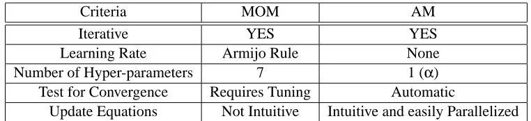
KL using MOM requires the careful tuning of a

number of extraneous parameters including, the learning rate (α) which is obtained using the Armijo rule which has 3 other parameters, MOM penalty parameter (c), stopping criteria (ζ), and penalty update parameters (γandβ). In general, in the interest of scalability, it is advantageous to have as few tuning parameters in an algorithm as possible, especially in the case of SSL where there is relatively little labeled data available to “hold out” for use in cross validation tuning. The success of MOM based optimization depends on the careful tuning of all the 7 extraneous parameters (this is in addition to µ and ν, the hyper-parameters in the original objective). This is problematic as settings of these parameters that yield good performance on a particular data set have no generalization guarantees. In Section 7.2.1, we present an analysis that shows sensitivity of MOM to the settings of these parameters.

2. Convergence guarantees: For most problems, MOM lacks convergence guarantees. Bert-sekas (1999) only provides a proof of convergence for cases when c(n)→∞, a condition rarely satisfied in practice.

3. Computational cost: The termination criteria for the MOM based solver for

P

KL requires

that one compute the value of the objective function for every iteration leading to increased computational complexity.

4. Lack of intuition in update equations: While the update equations for pi(y)are easy to obtain,

As stated above, there are other alternatives for numerical optimization of convex functions. In particular, we could use an IPM for solving

P

KL, but barrier methods also have their own drawbacks

(e.g., each step involves solving n linear equations). It is important to point out that we are not arguing against the use of gradient based approaches in general as they been quite successful for training multi-layer perceptrons, hidden conditional random fields, and so on where the objective is inherently non-convex. Sometimes even when the objective is convex, we need to rely on MOM or IPM for optimization like in our case in Section 9.2. However, as

P

KL is a convex optimization

problem, in this paper we explore and prefer other techniques for its optimization which do not have the aforementioned drawbacks.

4. Alternating Minimization (AM)

Given a distance function d(p,q)between objects p∈

P

,q∈

Q

where

P

,

Q

are sets, consider the problem finding the p,q that minimizes d(p,q). Sometimes solving this problem directly is hard, and in such cases the method of alternating minimization (AM) lends itself as a valuable tool for efficient optimization. AM refers to the case where we alternately minimize d(p,q)with respect to

p while q is held fixed and then vice-versa, that is,

p(n)=argmin

p∈P

d(p,q(n−1))and q(n)=argmin

q∈Q

d(p(n),q).

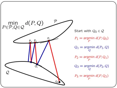
Figure 1 illustrates the two steps of AM over two convex sets. We start with an initial arbitrary

Q0∈

Q

which is held fixed while we minimize w.r.t. P∈

P

which leads to P1. The objective is

then held fixed w.r.t. P at P=P1 and minimized over Q∈

Q

and this leads to Q1. The above is

then repeated with Q1playing the role of Q0and so on until (in the best of cases) convergence. The

Expectation-Maximization (EM) (Dempster et al., 1977) algorithm is an example of AM. Moreover, the above objective over two variables can be extended to an objective over n variables. In such cases

n−1 variables are held fixed while the objective is optimized with respect to the one remaining variable and the procedure iterates in a similar round-robin fashion.

An AM procedure might or might not have the following properties: 1) a closed-form solution to each of the alternating minimization steps of AM; 2) convergence to a final solution, and 3) convergence to a correct minimum of d(p,q). In some cases, even when there is no closed-form solution to the direct minimization of d(p,q), each step of AM has a closed form solution. In other cases, however (see Corduneanu and Jaakkola, 2003), one or both the steps of AM do not have closed form solutions.

Depending on d(p,q)and on the nature of

P

,

Q

, an AM procedure might never converge. Even when AM does converge, it might not converge to the true correct minimum of d(p,q). In general, certain conditions need to hold for AM to converge to the correct solution. Some approaches, such as Cheney and Goldstien (1959), Zangwill (1969) and Wu (1983), rely on the topological properties of the objective and the space over which it is optimized, while others such as Csiszar and Tusnady (1984) use geometrical arguments. Still others (Gunawardena, 2001) use a combination of the above.

Q2

Q0

Q1

P1

P2

P3

Start withQ02 Q

P1= argmin

P d(P; Q0)

Q1= argmin

Q

d(P1; Q)

P2= argmin

P d(P; Q1)

Q2= argmin

Q d(P2; Q)

P3= argmin

P d(P; Q2)

min

P2P;Q2Qd(P; Q)

Figure 1: Alternating Minimization

Q0

P 2 P;8Q; Q₀

d(P; Q) +d(P; Q₀)

¸d(P; Q₁) +d(P₁; Q₁)

P₁= argmin

P

d(P; Q₀)

Q1= argmin Q

d(P1; Q)

P1

Q1

P

Q

Figure 2: Illustration of the 5-point property

Definition 3 IfP_, Q_{are convex sets of finite measures, given a divergence d(p,q), p∈}P_{, q∈}Q_,

then the 5-pp is said to hold for p∈P_if∀q,q0∈Q_{we have}

d(p,q) +d(p,q0)≥d(p,q1) +d(p1,q1)

where p1∈argmin

p∈P

d(p,q0)and q1∈argmin

q∈Q

d(p1,q).

Figure 2 shows an illustration of 5-pp. Here we start with some Q0∈

Q

, P1=argmin P∈P

d(P,Q0)

and Q1=argmin Q∈Q

d(P1,Q). 5-pp is said hold for d(P,Q)if for any P∈

P

and any Q∈

Q

, the sum

of the lengths of the red lines is greater than or equal to the sum of the lengths of the blue lines in Figure 2. Here the lengths are measured using the objective d(P,Q). Csiszar and Tusnady (1984) have shown that the 5-pp holds for all p when d(p,q) =DKL(p||q).

So now the question is whether our proposed objective

C

KL(p)can be optimized using AM and

4.1 Graph-based SSL using AM

P

KLcannot be solved using AM and so we reformulate it in a manner amenable to AM. The

follow-ing are the desired properties of such a reformulation –

1. The new (reformulated) objective should be a valid graph-based SSL criterion.

2. AM on the reformulated objective should converge to the global optimum of this objective.

3. The optimal solution in the case of the original (

P

KL) and reformulated problem should be

identical.

4. Each step of the AM process should have a closed form and easily computable solution.

5. The resulting algorithm should scale to large data sets.

In this section, we formulate an objective that satisfies all of these properties. Consider the following reformulated objective –

P

MP: min

p,q∈△m

C

MP(p,q)where

C

MP(p,q) =

l

∑

i=1

DKL ri||qi

+µ m

∑

i=1_j∈

∑

_N′_(i)

w′_{i j}DKL pi||qj

−ν

m

∑

i=1

H(pi)

where for each vertex i in

G

, we define a third discrete probability measure qiover the measurable

space(Y,

Y

), w′_{i j}=hW′

i i j, W

′

=W+αIn,

N

′

(i) ={i} ∪

N

(i)andα≥0. Here the qi’s play a

sim-ilar role as the pi’s and can potentially be used to obtain a final classification result (argmaxyqi(y)).

Thus, it would seem that we now have two classification results for each sample – one the most likely assignment according to pi and another given by qi. However,

C

MP includes terms of the

form(wii+α)DKL(pi||qi)which encourage piand qito be close to each other. Thusα, which is a

hyper-parameter, plays an important role in ensuring that pi=qi, ∀i. It should be clear that

argmin

p∈△n

C

KL(p) =αlim→∞argmin_p,q∈△n

C

MP(p,q).

In the following we will show that there exists a finiteαsuch that at a minima, pi(y) =qi(y)∀i,y

(henceforth we will denote this as either pi=qi ∀i or p=q).

We note that the new objective

C

MP(p,q)can itself be seen as an intrinsically valid SSL criterion.

While the first term encourages qifor the labeled vertices to be close to the labels, ri, the last term

encourages higher entropy p’s. The second term, in addition to acting as a graph regularizer, also acts as a glue between the p’s and q’s.

A natural question that arises at this point is why we choose this particular form for

C

MPand

not other alternatives. First note that−H(pi) =DKL(pi||u) +const where u is the uniform measure.

KLD is a function of two variables (say the left and the right). In

C

MP, the p’s always occur on the

left hand side while the q’s occur on the right. Recall that the reason

C

KL did not admit a closed

form solution is because we were attempting to optimize w.r.t. both the variables in a KLD. Thus going from

C

KL to

C

MP accomplishes two goals – (a) it makes optimization via AM possible, and

Lemma 4 If µ,ν,w′_{i j}≥0∀i,j then

C

MP(p,q)is convex.

Proof This follows as DKL(p||q) is convex in the pair, and we have a weighted sum of convex

functions with non-negative weights.

The previous lemma guarantees that any local minimum is a global minimum. The next theorem gives the powerful result that the AM procedure on our objective

C

MPis guaranteed to converge to

the true global minimum of

C

MP.

Theorem 5 (Convergence of AM on

C

MP, see appendix B) If

p(n)=argmin

p∈△m

C

MP

(p,q(n−1)), q(n)=argmin

q∈△m

C

MP

(p(n),q)and q(0)_i (y)>0∀y∈Y,∀i then

(a)

C

MP(p,q) +

C

MP(p,p(0))≥

C

MP(p,q(1)) +

C

MP(p(1),q(1))for all p,q∈△m, and (b) lim

n→∞

C

MP(p

(n)_,q(n)_{) =inf}

p,q∈△m

C

_MP(p,q).

Next we address the issue of showing that the solutions obtained in the case of the original and reformulated objectives are the same. We already know that ifα→∞then we have equality, but we are interested in obtaining a finite lower-bound onαfor which this is still the case. In the below, we let

C

MP(p,q;{wii′ =0}i)be the objective

C

MPshown with the weight matrix parameterized

with w′_ii=0 for all i, and we let

C

MP(p,q;α) be the objective function shown with a particular

parameterized value of α. For the proof of the next lemma and the two theorems that follow, see appendix C.

Lemma 6 We have that

min

p,q∈△m

C

MP(p,q; w

′

ii=0)≤_p∈min_△m

C

KL(p). Theorem 7 Given any A,B,S∈△m _{(i.e., A = [a}

1, . . . ,an], B= [b1, . . . ,bn], S= [s1, . . . ,sn]) such that ai(y),bi(y),si(y)>0, ∀ i,y and A6=B (i.e., not all ai(y) =bi(y)) then there exists a finiteα such that

C

MP(A,B)≥

C

MP(S,S) =

C

KL(S).

The above theorem states that there exists a finiteα that ensures

C

MP(p,q) evaluated on any

positive p6=q will be larger than any

C

KL(·). This is a stronger statement than we need, since we

are interested only in what happens at the objective functions’ minima. The following theorem does just this.

Theorem 8 (Equality of Solutions of

C

KLand

C

MP) Let

ˆp=argmin

p∈△m

C

KL(p)and(p

∗ ˜

α,q∗α˜) =argmin

p,q∈△m

C

MP(p,q; ˜α)

for an arbitrary ˜α>0 where p∗_α˜ = (p∗_{1; ˜α},· · ·,p∗_{m; ˜α})and q∗_α˜ = (q∗_{1; ˜α},· · ·,q∗_{m; ˜α}). Then there exists a finite ˆαsuch that at convergence of AM, we have that ˆp=p∗_αˆ =q∗_αˆ. Further, it is the case that if

p∗_α˜ 6=q∗_α˜, then

ˆ

α≥

C

KL(ˆp)−

C

MP(p

∗ ˜

α,q∗α˜;α=0) µ∑n_i=1DKL(p∗_{i; ˜α}||q∗_{i; ˜α})

We note that the above theorem guarantees the existence of a finiteαthat equates the minimum of

C

KL and

C

MPbut it does not say how to find it since we do not know the true optimum of

C

MP.

Nevertheless, if we use anαsuch that we end up with p∗=q∗(or in practice, approximately so) then we are assured that this is the true optimum for

C

KL.

As mentioned above, AM is not always guaranteed to have closed form updates at each step, but in our case closed form updates may be achieved. The AM updates (see Appendix E for the derivation) are given by

p(n)_i (y) = exp{

µ

γi∑jw

′ i jlog q

(n−1) j (y)}

∑yexp{_γµ_i∑jw′i jlog q (n−1) j (y)}

and

q(n)_i (y) =ri(y)δ(i≤l) +µ∑jw

′

jip (n)

j (y)

δ(i≤l) +µ∑jw

′

ji

whereγi=ν+µ∑jw

′

i j.

Thus,

C

MPsatisfies all the desired properties of the reformulation. In addition, it is also possible

to derive a test for convergence that does not require that one compute the value of

C

MP(p,q)(i.e.,

evaluate the objective).

Theorem 9 (Test for convergence, see Appendix D) If{(p(n),q(n))}∞_n=1is generated by AM of

C

MP(p,q) and

C

MP(p∗,q∗), inf

p,q∈△n

C

MP(p,q)then

C

MP(p(n),q(n))−

C

MP(p∗,q∗)≤ n

∑

i=1

δ(i≤l) +di

βi,

βi,log sup y

q(n)_i (y)

q(n−1)_i (y), dj=

∑

i wi j.

While a large number of optimization procedures resort to computing the change in the objective function with n (iteration index), in this case we have a simple check for convergence. This test does not require that one compute the value of the objective function which can be computationally expensive especially in the case of large graphs. Table 1 summarizes the advantages of the proposed AM approach to solving

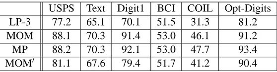
P

MP over that of using MOM to directly solve

P

KL. We also provide an

empirical comparison of these approaches in Section 7.2.1. Henceforth, we refer to the process of using AM to solve

P

MPas measure propagation (MP).

5. Squared-Loss Formulation

In this section, we show how the popular squared-loss objective may be formulated over measures. We then discuss its relationship to the proposed objective. Consider the optimization problem

P

SQ:

min

p∈△m

C

SQ(p)where

C

SQ(p) =

l

∑

i=1

kri−pik2+ m

∑

i=1j∈

∑

N(i)

wi jkpi−pjk2+ν m

∑

i=1

kpi−uk2

andkpk2_=∑

yp2(y).

P

SQcan also be seen as a multi-class extension of the quadratic cost criterion

Criteria MOM AM

Iterative YES YES

Learning Rate Armijo Rule None

Number of Hyper-parameters 7 1 (α)

Test for Convergence Requires Tuning Automatic

Update Equations Not Intuitive Intuitive and easily Parallelized

Table 1: There are two ways to solving the proposed objective, namely, the popular numerical op-timization tool method of multipliers (MOM), and the proposed approach based on alter-nating minimization (AM). This table compares the two approaches on various fronts.

Lemma 10 (Relationship between

C

KLand

C

SQ) We have that

C

KL(p)≥

C

SQ(p)

log 4 −mνlog|Y|.

Proof By Pinsker’s inequality we have that DKL(p||q) ≥ (1/log 4) ∑y|p(y)−q(y)| 2

≥

(1/log 4)∑_y|p(y)−q(y)|2_{. As a result}

C

KL(p) =

l

∑

i=1

DKL ri||pi

+µ m

∑

i=1j∈

∑

N(i)

wi jDKL pi||pj

−ν

m

∑

i=1

H(pi)

=

l

∑

i=1

DKL ri||pi

+µ m

∑

i=1j∈

∑

N(i)

wi jDKL pi||pj

+ν

m

∑

i=1

DKL(pi||u)−mνlog|Y|

≥ 1 log 4 " l

∑

i=1

kri−pik2+ m

∑

i=1j∈

∑

N(i)

wi jkpi−pjk2+ν m

∑

i=1

kpi−uk2 #

−mνlog|Y|

=

C

SQ(p)

log 4 −mνlog|Y|.

P

SQ can be reformulated as the following equivalent optimization problem

P

SQ: min p∈△m

C

SQ(p) where

C

SQ(p) =Tr (Sp−r′)(Sp−r′)T

+2µTr(LppT) +νTr((p−u)(p−u)T),

S,

Il 0

0 0

, r′,

r 0

0 0

, u,(u, . . . ,u)∈△m_,

1m∈Rm is a column vector of 1’s, and Il is the l×l identity matrix. Here L,D−W is the

unnormalized graph Laplacian, D is a diagonal matrix given by di= [D]ii=∑jwi j.

C

SQis convex if µ,ν≥0 and, as the constraints that ensure p∈△_{are linear, we can make use of the KKT conditions}

(Bertsekas, 1999) to show that the solution to

P

SQis given by

ˆp= (S+2µL+νIn)−1

Sr+νu+ 2µ

|Y|L1n1

T c

The above closed-form solution involves inverting a matrix of size m×m. Henceforth we refer to

the above closed form solution of

P

SQas SQ-Loss-C (C stands for closed form). Returning to the

original formulation, using Lagrange multipliers, setting the gradient to zero and solving for the multipliers we get the update for pi’s to be

p(n)_i (y) =ri(y)δ(i≤l) +νu(y) +µ∑jwi jp

(n−1) j (y)

δ(i≤l) +ν+µ∑_jwi j

. (1)

Here n is the iteration index. It can be shown that p(n)→ˆp (Bengio et al., 2007). In the following we refer to the iterative method of solving

P

SQas SQ-Loss-I. There has not been any work in the

past addressing the rate at which p(n)→ ˆp in the case of SQ-Loss-I. We address this issue in the following but first we define the rate of convergence of a sequence.

Definition 11 (Rate of Convergence Bertsekas, 1999 ) Let {xn} be a convergent sequence such that xn→0. It is said to have a linear rate of convergence if either

xn≤qηn∀n or limsup n→∞

xn

xn−1 ≤η

whereη∈(0,1)and q>0.

As “geometric” rate of convergence is a more appropriate description of linear convergence, we use this term in the paper.

Theorem 12 (Rate of Convergence for SQ-Loss, see Appendix D) If

(a) ν>0, and

(b) W has at least one non-zero off-diagonal element in every row (i.e., W is irreducible)

then the sequence of updates given in Equation 1 has a geometric rate of convergence for all i and y.

Thus we have that p(n)→ˆp very quickly. It is interesting to consider a reformulation of

C

SQin

a manner similar to

C

MP(see Section 4.1), as we do next.

5.1 AM Amenable Formulation of

P

SQ

Consider the following reformulation of

C

SQ

C

SQ′ (p,q) = l

∑

i=1

kri−qik2+

n

∑

i=1j∈

∑

N(i)

w′_{i j}kpi−qjk2+ν n

∑

i=1

kpi−uk2.

This form is amenable to AM and can be shown to satisfy 5-pp. Further the updates for two steps of AM have a closed form solution and are given by

p(n)_i (y) =νu(y) +µ∑jw

′ i jq

(n−1) j (y)

q(n)_i (y) =ri(y)δ(i≤l) +µ∑jw

′

jip (n)

j (y)

δ(i≤l) +µ∑jw

′

ji .

We call this method SQ-Loss-AM. It is important to point out that for solving

P

SQ, one always

resorts to either SQ-Loss-I or SQ-Loss-C depending on the nature of the problem. We will be using SQ-Loss-AM in the next section to provide more insights into the relationship between

P

KL and

P

SQ.

6. Connections to Other Approaches

In this section we explore connections between our proposed approach and other previously pro-posed SSL algorithms.

6.1 Squared-Loss Based Algorithms

A majority of previously proposed graph-based SSL algorithms (Zhu et al., 2003; Joachims, 2003; Belkin et al., 2005; Bengio et al., 2007) are based on minimizing squared-loss. In the following we refer to the squared-loss based SSL algorithm proposed in Zhu and Ghahramani (2002a) as label propagation (LP) (this is the standard version of label propagation, see Table 2), the algorithm in Zhu et al. (2003) as the harmonic functions algorithms (HF). Also QC denotes the quadratic cost criterion (Bengio et al., 2007). While the objectives used in the case of LP, HF and QC are similar in spirit to our

C

SQ, there are some important differences. In the case of both HF and QC, the objective

is defined over the reals whereas in our case

C

SQis defined over discrete probability measures. This

leads to two important benefits – (a) it allows easy generalization to multi-class problems, (b) it allows us to exploit well-defined functions of measures in order to improve performance. Further, both the HF and LP algorithms do not have guards against degenerate solutions (i.e., the third term in

C

SQ). QC, on the other hand, employs a regularizer similar to the third term in

C

SQbut QC is

limited to only two-class problems (for multi-class problems one resorts to one vs. rest). Both the LP and HF algorithms optimize the same objective but LP uses a iterative solution while HF employs the closed form solution (it has been shown that LP converges to the solution given by HF Zhu, 2005a). QC is a generalization of HF and has been shown to outperform it (Bengio et al., 2007). Our squared-loss formulation,

C

SQ, is a generalization of QC for multi-class problems and as we

show in Section 7.2.2, it outperforms QC. Thus, to compare against squared-loss based objectives, we simply use our formulation

C

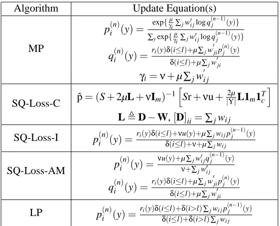
SQ.

Table 2 summarizes the update equations in the case of some of the graph-based SSL algorithms. It is interesting to compare the update equations for SQ-Loss-AM and MP. It can be seen that the update equations for qi(y)in the case of SQ-Loss-AM and MP are the same. In the case of MP, the pi(y)update may be re-written as

p(n)_i (y) = ∏j q

(n−1) j (y)

µw′_{i j}

∑y∏j q

(n−1) j (y)

µw′_{i j}.

Thus, while squared loss makes use of a weighted arithmetic-mean, MP uses a weighted geometric-mean to update pi(y). In other words, while squared-error leads to additive updates, the use of KLD

Algorithm Update Equation(s)

MP

p(n)_i (y) = exp{ µ

γi∑jw

′

i jlog q

(n−1)

j (y)}

∑yexp{_γµ i∑jw

′

i jlog q

(n−1)

j (y)}

q(n)_i (y) =ri(y)δ(i≤l)+µ∑jw

′

jip

(n)

j (y)

δ(i≤l)+µ∑jw

′

ji

γi=ν+µ∑jw

′

i j

SQ-Loss-C ˆp= (S+2µL+νIm)

−1h_Sr+νu+ 2µ |Y|L1m1Tc

i

L,D−W,[D]_ii=∑_jwi j

SQ-Loss-I _p(n)

i (y) =

ri(y)δ(i≤l)+νu(y)+µ∑jwi jp(jn−1)(y)

δ(i≤l)+ν+µ∑jwi j

SQ-Loss-AM p

(n) i (y) =

νu(y)+µ∑jw′i jq

(n−1)

j (y)

ν+∑jw′i j

q(n)_i (y) =ri(y)δ(i≤l)+µ∑jw

′

jip

(n)

j (y)

δ(i≤l)+µ∑jw

′

ji

LP _p(n)_i (y) =ri(y)δ(i≤l)+δ(i>l)∑jwi jp(jn−1)(y)

δ(i≤l)+δ(i>l)∑jwi j

Table 2: A summary of update equations for various graph-based SSL algorithms. MP stands for our proposed measure propagation approach, SQ-Loss-C, SQ-Loss-I and SQ-Loss-AM represent the closed-form, iterative and alternative-minimization based solutions for the objective based on squared-error. LP is label propagation (Zhu and Ghahramani, 2002a). In all cases µ andνare hyper-parameters.

Spectral graph transduction (SGT) (Joachims, 2003) is an approximate solution to the NP-hard norm-cut problem. The use of norm-cut instead of a mincut (as in Blum and Chawla, 2001) ensures that the number of unlabeled samples in each of the cuts is more balanced. SGT requires that one compute the eigen-decomposition of a m×m matrix which can be challenging for very large

data sets. Manifold regularization (Belkin et al., 2005) proposes a general framework in which a parametric loss function that is defined over the labeled samples and is regularized by graph smoothness term defined over both the labeled and unlabeled samples. When the loss function satisfies certain conditions, it can be shown that the representer theorem applies and so the solution is a weighted sum over kernel computations. Thus the goal of the learning process is to discover these weights. When the parametric loss function is based on least squares, the approach is referred to as

Laplacian regularized least squares (LapRLS) (Belkin et al., 2005) and when the loss function is

based on hinge loss, the approach is called Laplacian support vector machines (LapSVM)) (Belkin et al., 2005). In the case of LapRLS, the weights have a closed form solution which involves inverting a m×m matrix while in the case of LapSVM, optimization techniques used for SVM

So is there a reason to prefer KLD based loss over squared-error? In this context we quote two relevant statements from Bishop (1995)

1. Page 226: “ In fact, the sum-of-squares error function is not the most appropriate for

clas-sification problems. It was derived from maximum likelihood on the assumption of Gaussian distributed target data. However, the target values for a l-of-c coding scheme are binary, and hence far from having a Gaussian distribution.”

2. Page 235: “Minimization of the cross-entropy error function tends to result in similar relative

errors on both small and large target values. By contrast, the sum-of-squares error function tends to give similar absolute errors for each pattern, and will therefore give large relative errors for small output values. This suggests that the cross-entropy error function is likely to perform better than sum-of-squares at estimating small probabilities.”

While the above quotes were made in the context of a multi-layered perceptron (MLP), they apply to learning in general. While squared-error has worked well in the case of regression problems (Bishop, 1995),1for classification, it is often argued that squared-loss is not the optimal criterion and alternative loss functions such as the cross-entropy (Bishop, 1995), logistic (Ng and Jordan, 2002), hinge-loss (Vladimir, 1998) have been proposed. When attempting to measure the dissimilarity between measures, KLD is said to be asymptotically consistent w.r.t. the underlying probability distributions (Bishop, 1995). The second quote above furthers the case in favor of adopting KLD based loss as it is based on relative error rather absolute error as in the case of squared-error. In addition, KLD is an ideal measure for divergence of probability distributions as it has description-length consequences (coding with the wrong distribution will lead to longer description bit description-length than necessary). Most importantly, as we will show in Section 7, MP outperforms the squared-error based

P

SQon a number of tasks. We also present further empirical comparison of these two

objectives in Section 7.2.4.

We would like to note that Wang et al. (2008) proposed a graph-based SSL algorithm that also employs alternating minimization style optimization. However, it is inherently squared-loss based which MP outperforms (see Section 7). Further, they do not provide or state convergence guarantees and one side of their updates is not only not in the closed-form, but also it approximates an NP-complete optimization problem.

6.2 Information Regularization (Corduneanu and Jaakkola, 2003)

The information regularization (IR) (Corduneanu and Jaakkola, 2003) algorithm also makes use of a KLD based loss for SSL but is different from our proposed approach in following ways

1. IR is motivated from a different perspective. Here the input space is divided into regions

{Ri}which may or may not overlap. For a given point xj∈Ri, IR attempts to minimize the

KLD between pj(y|xj)and ˆpRi(y), the agglomerative distribution for region Ri. The intuition behind this is that, if a particular sample is a member of a region, then its posterior must be similar to the posterior of the other members. Given a graph, one can define a region to be a vertex and its neighbors thus making IR amenable to graph-based SSL. In Corduneanu and Jaakkola (2003), the agglomeration is performed by a simple averaging (arithmetic mean).

2. While IR suggests (without proof of convergence) the use of AM for optimization, one of the steps of the optimization does not admit a closed-form solution. This is a serious practical drawback especially in the case of large data sets.

3. It does not make use of a entropy regularizer. But as our results show, the entropy regularizer leads to much improved performance.

Tsuda (2005) (hereafter referred to as PD) is an extension of the IR algorithm to hyper-graphs where the agglomeration is performed using the geometric mean. This leads to closed form solutions in both steps of the AM procedure. However, like IR, PD does not make use of a entropy regularizer. Further, the update equation for one of the steps of the optimization in the case of PD (Equation 13 in Tsuda, 2005) is actually a special case of our update equation for pi(y)and may be obtained by

setting wi j=1/2. Further, our work here can be easily extended to hyper-graphs (see Section 9.3).

7. Results

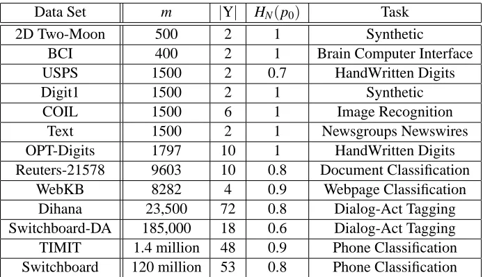
Table 3 lists the data sets that we use in this paper. These corpora come from a diverse set of domains, including image processing (handwritten digit recognition), natural language processing (document classification, webpage classification, dialog-act tagging), and speech processing (phone classification). The sizes vary from m=400 (BCI) to the largest data set, Switchboard, which has 120 million samples. The number of classes vary from|Y|=2 to|Y|=72 in the case of Dihana. The goal is to show that the proposed approach performs well on both small and large data sets, for binary and multi-class problems. Further, in each case we compare the performance of MP against the state-of-the-art algorithm for that task. Each data set is described in detail in the relevant sections.

7.1 Synthetic 2D Two-Moon Data Set

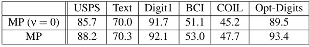
In order to understand the advantages of MP over other state-of-the-art SSL algorithms, we eval-uated their performance on the synthetic 2D two-moon data set. This is a binary classification problem. We compare against SQ-Loss-I (see Section 5), LapRLS (Belkin et al., 2005), and SGT (Joachims, 2003). For all approaches, we constructed a symmetrized 10-NN graph using an RBF kernel. In the case of LapRLS and SGT, the hyper-parameter values were set in accordance to the recipe in Belkin et al. (2005) and Joachims (2003) respectively. In the case of MP, we set µ=0.2,

ν=0.001 andα=1.0. For SQ-Loss-I, we set µ=0.2 andν=0.001. These values were found to give reasonable performance for most data sets.

Data Set m |Y| HN(p0) Task

2D Two-Moon 500 2 1 Synthetic

BCI 400 2 1 Brain Computer Interface

USPS 1500 2 0.7 HandWritten Digits

Digit1 1500 2 1 Synthetic

COIL 1500 6 1 Image Recognition

Text 1500 2 1 Newsgroups Newswires

OPT-Digits 1797 10 1 HandWritten Digits

Reuters-21578 9603 10 0.8 Document Classification

WebKB 8282 4 0.9 Webpage Classification

Dihana 23,500 72 0.8 Dialog-Act Tagging

Switchboard-DA 185,000 18 0.6 Dialog-Act Tagging

TIMIT 1.4 million 48 0.9 Phone Classification

Switchboard 120 million 53 0.8 Phone Classification

Table 3: List of Data Sets we used to compare the performance of various SSL algorithms.

HN(p0) =H(p0)/log|Y| is the normalized entropy of the prior and a value of 1 indi-cates a perfectly balanced data set while values closer to 0 imply imbalance. In the case of the Switchboard data set, HN(p0)was computed over the STP data (see Section 8.1).

-2 -1 0 1 2 3

-1 -0.5 0 0.5 1 1.5

-2 -1 0 1 2 3

-1 -0.5 0 0.5 1 1.5

-2 -1 0 1 2 3

-1 -0.5 0 0.5 1 1.5

-2 -1 0 1 2 3

-1 -0.5 0 0.5 1 1.5

-2 -1 0 1 2 3

-1 -0.5 0 0.5 1 1.5

-2 -1 0 1 2 3

-1 -0.5 0 0.5 1 1.5

-2 -1 0 1 2 3

-1 -0.5 0 0.5 1 1.5

-2 -1 0 1 2 3

-1 -0.5 0 0.5 1 1.5

-2 -1 0 1 2 3

-1 -0.5 0 0.5 1 1.5

-2 -1 0 1 2 3

-1 -0.5 0 0.5 1 1.5

-2 -1 0 1 2 3

-1 -0.5 0 0.5 1 1.5

-2 -1 0 1 2 3

-1 -0.5 0 0.5 1 1.5

1. MP is able to achieve perfect classification in the first two cases, and essentially perfect (2 errors) in the third case.

2. In the balanced case (first row), all approaches achieve perfect classification. Here, all ap-proaches are able to correctly learn the nature of the manifold.

3. In the imbalanced cases (second and third rows), all three other approaches (SQ-Loss-I, LapRLS, and SGT) fail to correctly classify a significant portion of samples. This is not surprising and has been observed by others in the past (see Figure 1 in Wang et al., 2008).

4. Finally, in the case of SQ-Loss-I, we tried using class mass normalization (CMN) (Zhu and Ghahramani, 2002a) as a post-processing step. While the results did not change in the bal-anced case, CMN in fact resulted in worse error rate performance in the imbalbal-anced cases. Note that Figure 3 for SQ-Loss-I does not include CMN.

7.2 Results on Benchmark SSL Data Sets

We also evaluated the performance of MP on a number of benchmark SSL data sets including, USPS, Text, Digit1, BCI, COIL and Opt-Digits. All the above data sets, with the exception of Opt-Digits (obtained from the UCI machine learning repository), came from http://www.kyb. tuebingen.mpg.de/ssl-book. Digit1 is a synthetic data set, USPS is a handwritten digit recog-nition task, BCI involves classifying signals obtained from a brain computer interface, COIL is a part of the Columbia object image recognition library and involves classifying objects using images taken at different orientations. Text involves classifying IBM vs. the rest for documents taken from the top 5 categories in comp.* newswire. Opt-Digits is also a handwritten digit recognition task. We note that most of these data sets are perfectly balanced (see Table 3)—further details may be found in Chapelle et al. (2007).

We compare MP against four other algorithms: 1) k-nearest neighbors; 2) Spectral Graph Trans-duction (SGT) (Joachims, 2003); 3) Laplacian Regularized Least Squares (LapRLS) (Belkin et al., 2005); and 4)

P

SQ solved using SQ-Loss-I. Here k-nearest neighbors is the fully-supervised

ap-proach, while others are graph-based SSL approaches. We used the standard features supplied with the corpora without any further processing. For the graph-based approaches we constructed sym-metrized k-NN graphs using an RBF kernel. We discuss the choice of k and the width of the kernel shortly. For each data set, we generated transduction sets with different number of labeled samples,

l∈ {10,20,50,80,100,150}. In each case, we generated 11 different transduction sets. The first set was used to tune the hyper-parameters which were then held fixed over the remaining sets. In the case of the k-nearest neighbors approach, we tried k∈ {1,2,4,5,10,20,30,40,50,70,90,100,120,

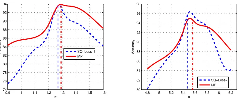
140,150,160,180,200}. For the graph-based approaches, k (for the k-NN graph) was tuned on the first transduction set over the following values k∈ {2,5,10,50,100,200,m}. The optimal width of the RBF kernel,σ, in the case of SQ-Loss-I, SGT and MP was determined over the following set

σ∈ {ga/3 : a∈ {2,3,· · ·,10}} where ga is the average distance between each sample and its ath

nearest neighbor over the entire data set (Bengio et al., 2007).

In the case of LapRLS, we followed the setup described in Section 21.2.5 of Chapelle et al. (2007). Here, as per the recipe in Joachims (2003), the optimalσwas determined in a slightly differ-ent manner—we triedσ∈ {σ0

8,σ

0

4,σ

0

2,σ0,2σ0,4σ0,8σ0}whereσ0is the average norm of the feature

vectors. In addition the hyper-parametersγA, r (see Belkin et al., 2005) associated with LapRLS

USPS Digit1

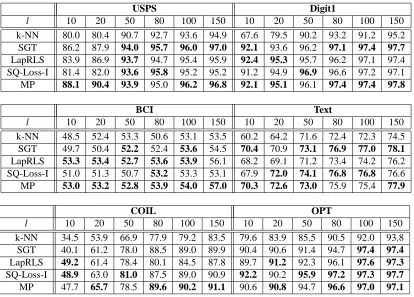
l 10 20 50 80 100 150 10 20 50 80 100 150

k-NN 80.0 80.4 90.7 92.7 93.6 94.9 67.6 79.5 90.2 93.2 91.2 95.2

SGT 86.2 87.9 94.0 95.7 96.0 97.0 92.1 93.6 96.2 97.1 97.4 97.7

LapRLS 83.9 86.9 93.7 94.7 95.4 95.9 92.4 95.3 95.7 96.2 97.1 97.4

SQ-Loss-I 81.4 82.0 93.6 95.8 95.2 95.2 91.2 94.9 96.9 96.6 97.2 97.1

MP 88.1 90.4 93.9 95.0 96.2 96.8 92.1 95.1 96.1 97.4 97.4 97.8

BCI Text

l 10 20 50 80 100 150 10 20 50 80 100 150

k-NN 48.5 52.4 53.3 50.6 53.1 53.5 60.2 64.2 71.6 72.4 72.3 74.5

SGT 49.7 50.4 52.2 52.4 53.6 54.5 70.4 70.9 73.1 76.9 77.0 78.1

LapRLS 53.3 53.4 52.7 53.6 53.9 56.1 68.2 69.1 71.2 73.4 74.2 76.2

SQ-Loss-I 51.0 51.3 50.7 53.2 53.3 53.1 67.9 72.0 74.1 76.8 76.8 76.6

MP 53.0 53.2 52.8 53.9 54.0 57.0 70.3 72.6 73.0 75.9 75.4 77.9

COIL OPT

l 10 20 50 80 100 150 10 20 50 80 100 150

k-NN 34.5 53.9 66.9 77.9 79.2 83.5 79.6 83.9 85.5 90.5 92.0 93.8

SGT 40.1 61.2 78.0 88.5 89.0 89.9 90.4 90.6 91.4 94.7 97.4 97.4

LapRLS 49.2 61.4 78.4 80.1 84.5 87.8 89.7 91.2 92.3 96.1 97.6 97.3

SQ-Loss-I 48.9 63.0 81.0 87.5 89.0 90.9 92.2 90.2 95.9 97.2 97.3 97.7

MP 47.7 65.7 78.5 89.6 90.2 91.1 90.6 90.8 94.7 96.6 97.0 97.1

Table 4: Comparison of accuracies for different number of labeled samples (l) across USPS, Digit1, BCI, Text, COIL and Opt-Digits data sets. In each column, the best performing system and all approaches that are not significantly different at the 0.001 level (according to the difference of proportions significance test) are shown bold-faced.

1e4, 1e6}. Also, as per Belkin et al. (2005), we set p=5 in the case of Text data set and p=2 for all the other data sets. In the case of SGT, the search was over c∈ {3000, 3200, 3400, 3800, 5000, 100000}(Joachims, 2003). Finally, the trade-off parameters, µ andν(associated with both MP and SQ-Loss-I) were tuned over the following sets: µ∈ {1e–8, 1e–6, 1e–4, 1e–2, 0.1, 1, 10}

andν∈ {1e–8, 1e–6, 1e–4, 1e–2, 0.1}. In the case of SQ-Loss-I, the results were obtained after the application of CMN as a post-processing step as this has been shown to be beneficial to the performance on benchmark data sets (Chapelle et al., 2007). For MP, we initialized p(0) such that all assignments had non-zero probability mass as this is a required condition for convergence and setα=1. As LapRLS and SGT assume binary classification problems, results for the multi-class data sets (COIL and OPT) were obtained using one vs. rest.

The mean accuracies over the 10 transduction sets (i.e., excluding the set used for tuning the hyper-parameters) for each corpora is shown in Table 4. The following observations may be made from these results