Bayesian Leave-One-Out Cross-Validation Approximations
for Gaussian Latent Variable Models
Aki Vehtari [email protected]
Tommi Mononen Ville Tolvanen Tuomas Sivula
Helsinki Institute of Information Technology HIIT, Department of Computer Science, Aalto University P.O.Box 15400, 00076 Aalto, Finland
Ole Winther [email protected]
Technical University of Denmark DK-2800 Lyngby, Denmark
Editor:Kevin Murphy
Abstract
The future predictive performance of a Bayesian model can be estimated using Bayesian cross-validation. In this article, we consider Gaussian latent variable models where the integration over the latent values is approximated using the Laplace method or expectation propagation (EP). We study the properties of several Bayesian leave-one-out (LOO) cross-validation approximations that in most cases can be computed with a small additional cost after forming the posterior approximation given the full data. Our main objective is to assess theaccuracy of the approximative LOO cross-validation estimators. That is, for each method (Laplace and EP) we compare the approximate fast computation with the exact brute force LOO computation. Secondarily, we evaluate the accuracy of the Laplace and EP approximations themselves against a ground truth established through extensive Markov chain Monte Carlo simulation. Our empirical results show that the approach based upon a Gaussian approximation to the LOO marginal distribution (the so-called cavity distribution) gives the most accurate and reliable results among the fast methods.
Keywords: predictive performance, leave-one-out cross-validation, Gaussian latent vari-able model, Laplace approximation, expectation propagation
1. Introduction
Bayesian cross-validation can be used to assess predictive performance. Vehtari and Ojanen (2012) provide an extensive review of theory and methods in Bayesian predictive performance assessment including decision theoretical assumptions made in Bayesian cross-validation. Gelman et al. (2014) provide further details on theoretical properties of leave-one-out cross-validation and information criteria, and Vehtari et al. (2016) provide practical fast computation in the case of Monte Carlo posterior inference. In this article, we present the properties of several Bayesian leave-one-out (LOO) cross-validation approximations for
latent variables is performed with either the Laplace method or expectation propagation (EP). We show that for these methods leave-one-out cross-validation can be computed accurately with zero or a negligible additional cost after forming the full data posterior approximation.
Global (Gaussian) and factorizing variational approximations for latent variable inference are not considered in this paper. They have the same order computational complexity as Laplace and EP but with a larger pre-factor on the dominatingO(n3) term, where nis the number of observations (Nickisch and Rasmussen, 2008). EP may be expected to be the most accurate method (e.g. Nickisch and Rasmussen, 2008; Vanhatalo and Vehtari, 2010; Jyl¨anki et al., 2011; Riihim¨aki et al., 2013) and Laplace to have the smallest computational overhead. So EP and Laplace may be considered the methods of choice for accuracy and speed, respectively. We expect that our overall results and conclusions for Laplace and EP carry over to Gaussian variational. For non-GLVM models such as generalized linear and deep generative models, the (factorized) Gaussian variational approximations scale to large data sets (Challis and Barber, 2013; Ranganath et al., 2014; Kingma and Welling, 2014; Rezende et al., 2014). It is of interest to derive approximate LOO estimators for these models, but that is outside the scope of this paper.
We consider a prediction problem with an explanatory variablexand an outcome variable
y. The same notation is used interchangeably for scalar and vector-valued quantities. The observed data are denoted by D = {(xi, yi)}ni=1 and future observations by (˜x,y˜). We
focus on GLVMs, where the observation modelp(yi|fi, φ) depends on a local latent value fi and possibly on some global parametersφ, such as the scale of the measurement error
process. Latent valuesf = (f1, . . . , fn) have a joint Gaussian priorp(f|x, θ) which depends
on covariatesx and hyperparametersθ(e.g., covariance function parameters for a Gaussian process). The posterior of the latent f is then
p(f|D, θ, φ)∝p(f|x, θ)
n
Y
i=1
p(yi|fi, φ). (1)
As a specific example we use Gaussian process (GP) models (reviewed, e.g., by Rasmussen and Williams, 2006), but the methods are applicable also for other GLVMs which have the same factorizing form (e.g. Gaussian Markov random field models used in the R-INLA software (Lindgren and Rue, 2015)). Some of the presented methods are applicable more generally, requiring only a factorizing likelihood with terms p(yi|fi, φ) and a method to
integrate over the marginal posteriorsp(fi|D, θ, φ). The results presented in this paper can
be generalized to the cases where a likelihood term depends upon more than one latent variable (e.g. Tolvanen et al., 2014) or the latent value prior is non-Gaussian (e.g. Seeger, 2008; Hern´andez-Lobato et al., 2008; Hern´aandez-Lobato et al., 2010). For clarity we restrict our treatment to the case of one likelihood term with one latent value.
The predictive distribution for a future observation ˜y given future covariate values ˜x is
p(˜y|x, D˜ ) =
Z
p(˜y|f , φ˜ )p( ˜f|x, D, θ˜ )p(φ, θ|D)df dφdθ.˜ (2)
The expected predictive performance using the log score and unknown true distribution of the future observation pt(˜x,y˜) is
Z
pt(˜x,y˜) logp(˜y|x, D˜ )dxd˜ y.˜ (3)
This expectation can be approximated by re-using the observations and computing the leave-one-out Bayesian cross-validation estimate
LOO = 1
n n
X
i=1
logp(yi|xi, D−i), (4)
where D−i is all other observations except (xi, yi). Here we consider only cases with random
˜
x from the same distribution asx. See Vehtari and Ojanen (2012) for discussion of fixed, shifted, deterministic, or constrained ˜x.
In addition to estimating the expected log predictive density, it may be interesting to look at a single value, logp(yi|xi, D−i). These terms, also called conditional predictive
ordinates (CPOi), may reveal observations which are highly influential or not well explained
by the model (see, e.g., Gelfand, 1996). The probability integral transform (PIT) values
F(yi|xi, D−i), whereF is the predictive CDF, can be used to assess the calibration of the
predictions (see, e.g., Gneiting et al., 2007).
The straightforward brute force implementation of leave-one-out cross-validation requires recomputing the posterior distribution n times. Often leave-one-out cross-validation is replaced withk-fold cross-validation requiring only krecomputations of the posterior, with
k usually 10 or less. Although k-fold-CV is robust and would often be computationally feasible, there are several fast approximations for computing LOO with a negligible additional computational cost after forming the posterior with the full data.
Several studies have shown that the Laplace method and EP perform well (compared to the gold standard Markov chain Monte Carlo inference) for GLVMs with many log-concave likelihoods (e.g. Rue et al., 2009; Vanhatalo et al., 2010; Martins et al., 2013; Riihim¨aki and Vehtari, 2014). EP has also been shown to be close to Markov chain Monte Carlo inference for classification models (log-concave likelihood, but potentially highly skewed posterior) and non-log-concave likelihoods (e.g. Nickisch and Rasmussen, 2008; Vanhatalo and Vehtari, 2010; Jyl¨anki et al., 2011; Cseke and Heskes, 2011; Riihim¨aki et al., 2013; Vanhatalo et al., 2013; Tolvanen et al., 2014). In this paper we also consider the accuracy of approximative LOO with standard Markov chain Monte Carlo inference for LOO as our benchmark.
In practical data analysis work, it is useful to start with fast approximations and step by step check whether a computationally more expensive approach can improve the predictive accuracy. We propose the following three step approach:
2. Using ( ˆφ,θˆ) obtained in the previous step, use EP to integrate over the latent values and check whether the predictive performance improves substantially compared to using the Laplace method (we may also re-estimate ˆφand ˆθ).
3. Integrate over φandθ and check whether integration over the parameters improves predictive performance.
Details of the computations involved are given in Sections 2 and 3. Based on these steps we can continue with the model that has the best predictive performance or the one that makes predictions fastest, or both. Often we also need to re-estimate models when data are updated or additional covariates become available, and then again a fast and accurate posterior approximation is useful. To follow the above approach, we need accurate predictive performance estimates for the Laplace method and EP.
The main contributions of this paper are:
• A unified presentation and thorough empirical comparison of methods for approximate LOO for Gaussian latent variable models with both log-concave and non-log-concave likelihoods and MAP and hierarchical approaches for handling hyperparameter inference (Section 3).
• The main conclusion from the empirical investigation (Section 4) is the observed superior accuracy/complexity tradeoff of Gaussian latent cavity distribution based LOO estimators. Although there are more accurate non-Gaussian approximations of the marginal posteriors, their use does not translate into substantial improvements in terms of LOO cross-validation accuracy and also introduces considerable instability. Using the widely applicable information criterion (WAIC) in the computation does not provide any benefits.
• The Laplace Gaussian cavity distribution (LA-LOO) (Section 3.5), although mentioned by Cseke and Heskes (2011), has not been used previously for LOO estimation. LOO consistency of LA-LOO using linear response theory is proved (Appendix A).
• Truncated weights quadrature integration (Section 3.7) inspired by truncated im-portance sampling is a novel way to stabilize the quadrature used in some LOO computations.
2. Gaussian Latent Variable Models
In this section, we briefly review the notation and methods for Gaussian latent variable models used in the rest of the article. We focus on Gaussian processes (see, e.g., Rasmussen and Williams, 2006), but most of the discussion also holds for other factorizing GLVMs. We consider models with a Gaussian prior p(f|x, θ) on latent values f = (f1, . . . , fn) and
factorizing likelihood
p(f|D, θ, φ) = 1
Z n
Y
i=1
where Z is a normalization factor and equal to the marginal likelihood p(y|X, θ, φ) =
R Qn
i=1p(yi|fi, φ)p(f|X, θ)df. For example, in the Gaussian process framework the
multi-variate Gaussian prior on latent values isp(f|x, θ) = N(f|µ0, K), whereµ0 is the prior mean
andK is a covariance matrix constructed by a covariance functionKi,j =k(xi, xj;θ), which
characterizes the correlation between two points. In this paper, we assume that the prior mean µ0 is zero, but the results generalize to nonzero prior means as well.
2.1 Gaussian Observation Model
With a Gaussian observation model,
p(yi|fi, σ2) = N(yi|fi, σ2), (6)
where φ = σ2 is the noise variance, the conditional posterior of the latent variables is a multivariate Gaussian
p(f|D, θ, φ) = N(f|µ,Σ),
where µ=K(K+σ2I)−1y
and Σ = (K−1+σ−2I)−1=K−K(K+σ2I)−1K. (7) The marginal posterior is simply p(fi|D, θ, σ2) = N(µi,Σii) and the marginal likelihood p(y|X, θ, σ2) can be computed analytically using properties of the multivariate Gaussian
(see, e.g., Rasmussen and Williams, 2006).
2.2 Non-Gaussian Observation Model
In the case of a non-Gaussian likelihood, the conditional posteriorp(f|D, θ, φ) needs to be approximated. In this paper, we focus on expectation propagation (EP) and the Laplace method (LA), which form a multivariate Gaussian approximation of the joint latent posterior
q(f|D, θ, φ) = 1
Zp(f|X, θ) n
Y
i=1
˜
ti(fi), (8)
where the ˜ti are (unnormalized) Gaussian approximations of the likelihood contributions.
We useq to denote approximative joint and marginal distributions in general, or the specific approximation used in each case can be inferred from the context.
2.3 Expectation Propagation
Expectation propagation (Opper and Winther, 2000; Minka, 2001) approximates independent non-Gaussian likelihood terms by unnormalized Gaussian form site approximations (aka pseudo-observations),
where ˜Zi =
R
p(yi|fi) N(fi|µ˜i,Σ˜i)dfi, and ˜µi and ˜Σi are the parameters of the site
approxi-mations, or site parameters. The joint latent posterior approximation is then
p(f|D, φ, θ) = 1
Zp(f|X, θ) Y
i
p(yi|fi, φ)
≈ 1
ZEP
p(f|X, θ)Y
i
˜
ti(fi) =q(f|D, φ, θ), (10)
where Z is the normalization constant or the marginal likelihood, ZEP is the EP
ap-proximation to the marginal likelihood and q(f|D) is a multivariate Gaussian posterior approximation.
EP updates the site approximations by iteratively improving accuracy of the marginals. To update the ith site approximation, it is first removed from the marginal approximation to form a cavity distribution,
q−i(fi)∝q(fi|D)/t˜i(fi), (11)
where the marginal q(fi|D) is obtained analytically using properties of the multivariate
Gaussian.
The cavity distribution is combined with the original likelihood term to form a more accurate marginal distribution called the tilted distribution:
q−i(fi)p(yi|fi, φ). (12)
Minimization of Kullback-Leibler divergence from the tilted distribution to the marginal approximation corresponds to matching the moments of the distributions. Hence for Gaussian approximation, the zeroth, first and second moments of this tilted distribution are computed, for example, using one-dimensional numerical integration. The site parameters are updated so that moments of the marginal approximation q(fi|D) match the moments of
the tilted distribution q−i(fi)p(yi|fi, φ). The newq(f) can be computed after a single site
approximation has been updated (sequential EP) or after all the site approximations have been updated (parallel EP).
2.4 Laplace Approximation
The Laplace approximation is constructed from the second-order Taylor expansion of logp(f|y, θ, φ) around the mode ˆf, which gives a Gaussian approximation to the conditional posterior,
q(f|D, θ, φ) = N(f|f ,ˆΣ)ˆ ≈p(f|D, θ, φ), (13)
where ˆΣ = (K−1+ ˜Σ−1)−1 is the inverse of the Hessian at the mode with ˜Σ being a diagonal matrix with elements (e.g., Rasmussen and Williams, 2006; Gelman et al., 2013),
˜ Σi =−
1
∇i∇ilogp(yi|fi, φ)|f
i= ˆfi
From this joint Gaussian approximation we can analytically compute an approximation of the marginal posterior p(fi|D, θ, φ) and the marginal likelihood p(y|x, θ, φ). The Laplace
approximation can also be written as
q(f|D, θ, φ) = 1
Zp(f|X, θ) n
Y
i=1
˜
ti(fi), (15)
where ˜ti(fi) are Gaussian terms N(fi|µ˜i,Σ˜i) with
˜
µi = ˆf + ˜Σi∇ilogp(yi|fi, φ)|f
i= ˆfi. (16)
2.5 Marginal Posterior Approximations
Many leave-one-out approximation methods require explicit computation of full posterior marginal approximations. We thus review alternative Gaussian and non-Gaussian approxi-mations of the marginal posteriorsp(fi|D, θ, φ) following the article by Cseke and Heskes
(2011). The exact joint posterior can be written as (droppingθ,φ and Dfor brevity)
p(f)∝q(f)Y
i
i(fi) with i(fi) =p(yi|fi, φ)/˜ti(fi), (17)
wherei(fi) is the ratio of the exact likelihood and the site term approximating the likelihood.
By integrating over the other latent variables, the marginal posterior can be written as
p(fi)∝q(fi)i(fi)
Z
q(f−i|fi)
Y
j6=i
j(fj)df−i
| {z }
ci(fi)
, (18)
where f−i represents all other latent variables except fi. Local methods usei(fi) which
depends locally only on fi. Global methods additionally use an approximation of ci(fi)
which depends globally on all latent variables. Next we briefly review different marginal posterior approximations of this exact marginal (see Table 1 for a summary).
2.5.1 Gaussian Approximations
The simplest approximation is to use the Gaussian marginals q(fi), which are easily obtained
from the joint Gaussian obtained by the Laplace approximation or expectation propagation; we call these LA-G and EP-G. By denoting the mean and variance of the pseudo observations (defined by the site terms) by ˜µi and ˜σi2 respectively, the joint approximation has the same
form as in the Gaussian case:
q(f|D, θ, φ) = N(µ,Σ)
Method Improvement Explanation
LA-G - Gaussian marginalq(fi) from the joint distribution
LA-L local tilted distributionq(fi)˜ti(fi)−1p(yi|fi, φ)
LA-TK global q(fi)˜ti(fi)−1p(yi|fi, φ)ci(fi), where ci(fi) is approxi-mated using the Laplace approximation
LA-CM/CM2/FACT global q(fi)˜ti(fi)−1p(yi|fi, φ)ci(fi), where ci(fi) is approxi-mated using the Laplace approximation with simpli-fications
EP-G - Gaussian marginalq(fi) from the joint distribution
EP-L local tilted distributionq−i(fi)p(yi|fi, φ), where q−i(fi) is ob-tained as a part of EP method
EP-FULL global q−i(fi)p(yi|fi, φ)ci(fi), whereci(fi) is approximated us-ing EP
EP-1STEP/FACT global q−i(fi)p(yi|fi, φ)ci(fi), whereci(fi) is approximated us-ing EP with simplifications
Table 1: Summary of the methods for computing approximate marginal posteriors. In global methods ci(fi) =
R
q(f−i|fi)Qj=6 ij(fj)df−i is a multivariate integral and j(fj) =p(yj|fj, φ)/˜tj(fj).
2.5.2 Non-Gaussian Approximations Using a Local Correction
The simplest improvement to Gaussian marginals is to include the local term i(fi), and
assume that the global term ci(fi) ≈ 1. For EP the result is the tilted distribution q(fi)i(fi) =q−i(fi)p(yi|fi, φ) which is obtained as a part of the EP algorithm (Opper and
Winther, 2000). As only the local terms are used to compute the improvement, Cseke and Heskes (2011) refer to it as the local improvement and denote the locally improved EP marginal as EP-L.
For the Laplace approximation, Cseke and Heskes (2011) propose a similar local improve-ment LA-L which can be written asq(fi)˜ti(fi)−1p(yi|fi, φ), where the site approximation
˜
ti(fi) is based on the second order approximation of logp(yi|fi, φ) (see Section 2.4). In
Section 3.5, we propose an alternative way to compute the equivalent marginal improvement using a tilted distribution q−i(fi)p(yi|fi, φ), where the cavity distribution q−i(fi) is based
on a leave-one-out formula derived using linear response theory (Appendix A). The local methods EP-L and LA-L can improve the marginal posterior approximation only at the observedx, and the marginal posterior at new ˜xis the usual Gaussian predictive distribution.
2.5.3 Non-Gaussian Approximations Using a Global Correction
Global approximations also take into account the global term ci(fi) by approximating
the multidimensional integral in Equation (18), again using Laplace or EP. To obtain an approximation for the marginal distribution, the integral ci(fi) has to be evaluated with
used. Global methods can be used to obtain an improved non-Gaussian posterior marginal approximation also at the not yet observed ˜x.
Using the Laplace approximation to evaluate ci(fi) corresponds to an approach proposed
by Tierney and Kadane (1986), and so we label the marginal improvement as LA-TK. Rue et al. (2009) proposed an approach that can be seen as a compromise between the computationally intensive LA-TK and the local approximation LA-L. Instead of finding the mode for eachfi, they evaluate the Taylor expansion around the conditional mean obtained
from the joint approximation q(f). The method is referred to as LA-CM. Cseke and Heskes (2011) propose the improvement LA-CM2 which adds a correction to take into account that the Taylor expansion is not done at the mode. To further reduce the computational effort, Rue et al. (2009) propose additional approximations with performance somewhere between LA-CM and LA-L. Rue et al. (2009) also discuss computationally efficient schemes for selecting values of fi and interpolation or parametric model fitting to estimate the marginal
density for other values offi. Cseke and Heskes (2011) propose similar approaches for EP,
with EP-FULL corresponding to LA-TK, and EP-1STEP corresponding to LA-CM/LA-CM2. Cseke and Heskes (2011) also propose EP-FACT and LA-FACT which use factorized approximation to speed up the computation of the normalization terms.
The local improvements EP-L and LA-L are obtained practically for free and all global approximations are significantly slower. See Appendix B for the computational complexities of the global approximations. Based on the results by Cseke and Heskes (2011), EP-L is inferior to global approximations, but the difference is often small, and LA-L is often worse than the global approximations. Also based on the results by Cseke and Heskes (2011) and our own experiments, we chose to use LA-CM2 and EP-FACT as the global corrections in the experiments.
2.6 Integration Over the Parameters
To marginalize out the parameters θ and φ from the previously mentioned conditional posteriors, we can use the exact or approximated marginal likelihood p(y|x, θ, φ) to form the marginal posterior for the parameters
p(θ, φ|D)∝p(y|X, θ, φ)p(θ, φ), (20)
and use numerical integration to integrate over θand φ. Commonly used methods include various Monte Carlo algorithms (see list of references in Vanhatalo et al., 2013) as well as deterministic procedures, such as the central composite design (CCD) method by Rue et al. (2009). Using stochastic or deterministic samples, the marginal posterior can be approximated as
p(f|D)≈
S
X
s=1
p(f|D, φs, θs)ws, (21)
where ws is a weight for the sample (φs, θs).
Method Based on
IS-LOO importance sampling / importance weighting, Section 3.6
Q-LOO quadrature integration, Section 3.7
TQ-LOO truncated quadrature integration, Section 3.7
LA-LOO same as Q-LOO with LA-L, Section 3.5
EP-LOO same as Q-LOO with EP-L, obtained as byproduct of EP, Section 3.4
WAICG matches the first two terms of the Taylor series expansion of LOO, Section 3.8 WAICV matches the first three terms of the Taylor series expansion of LOO, Section 3.8
Table 2: Summary of the leave-one-out (LOO) cross-validation approximations reviewed.
3. Leave-One-Out Cross-Validation Approximations
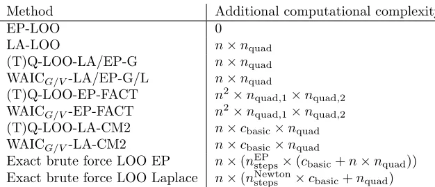
We start by reviewing the generic exact LOO equations, which are then used to provide a unifying view of the different approximations in the subsequent sections. We first review some special cases and then more generic approximations. The LOO approximations and their abbreviations are listed in Table 2. The computational complexities of the LOO approximations have been collected in Appendix B.
3.1 LOO from the Full Posterior
Consider the case where we have not yet seen theith observation. Then using Bayes’ rule we can add information from the ith observation:
p(fi|D) =
p(yi|fi)p(fi|xi, D−i) p(yi|xi, D−i)
, (22)
again droppingφ and θ for brevity. Correspondingly we can remove the effect of the ith observation from the full posterior:
p(fi|xi, D−i) =
p(fi|D)p(yi|xi, D−i) p(yi|fi)
(23)
If we now integrate both sides overfi and rearrange the terms we get
p(yi|xi, D−i) = 1/
Z
p(fi|D) p(yi|fi)
dfi. (24)
In theory this gives the exact LOO result, but in practice we usually need to approximate
p(fi|D) and the integral over fi. In the following sections we first discuss the hierarchical
approach, then the analytic, Monte Carlo, quadrature, WAIC, and Taylor series approaches for computing the conditional version of Equation (24). We then consider how the different marginal posterior approximations affect the result.
In some cases, we can compute p(fi|xi, D−i) exactly or approximate it efficiently and
then we can compute the LOO predictive density foryi,
p(yi|xi, D−i) =
Z
Or, if we are interested in the predictive distribution for a new observation ˜yi, we can
compute
p(˜yi|xi, D−i) =
Z
p(˜yi|fi)p(fi|xi, D−i)dfi, (26)
which is evaluated with different values of ˜yi as it is not fixed likeyi.
3.2 Hierarchical Approximations
Instead of approximating the leave-one-out predictive density p(yi|xi, D−i) directly, for
hierarchical models such as GLVMs it is often easier to first compute the leave-one-out predictive density conditional on the parameters p(yi|xi, D−i, θ, φ), then compute the
leave-one-out posteriors for the parametersp(θ, φ|D−i) and combine the results
p(yi|xi, D−i) =
Z
p(yi|xi, D−i, θ, φ)p(θ, φ|D−i)dθdφ. (27)
Sometimes the leave-one-out posterior of the hyperparameters is close to the full posterior, that is,p(θ, φ|D−i)≈p(θ, φ|D). The joint leave-one-out posterior can be then approximated
as
p(fi|xi, D−i)≈
Z
p(fi|xi, D−i, θ, φ)p(θ, φ|D)dθdφ (28)
(see, e.g., Marshall and Spiegelhalter, 2003). This approximation is a reasonable alternative if removing (xi, yi) has only a small impact onp(θ, φ|D) but a larger impact onp(fi|D, φ, θ).
Furthermore, if the posterior p(θ, φ|D) is narrow, a Type II MAP point estimate of the parameters ˆφ,θˆmay produce similar predictions as integrating over the parameters,
p(fi|xi, D−i)≈p(fi|xi, D−i,θ,ˆ φˆ). (29)
3.3 LOO with Gaussian Likelihood
If bothp(yi|fi, φ) and p(f|θ) are Gaussian, then we can compute p(fi|xi, D−i) analytically.
Starting from the marginal posterior we can remove the contribution of theith factor in the likelihood:
p(fi|xi, D−i, θ, φ)∝
p(fi|D, θ) p(yi|fi, φ)
= N(fi|µ−i, v−i), (30)
where
µ−i=v−i(Σii−1µi−σ−2yi) v−i= Σ−ii1−σ−2
−1
. (31)
These equations correspond to the cavity distribution equations in EP.
Sundararajan and Keerthi (2001) derived the leave-one-out predictive distribution
partitioned matrices. This gives a numerically alternative but mathematically equivalent way to compute the leave-one-out posterior mean and variance:
µ−i =yi−c¯−ii1gi
v−i = ¯c−ii1−σ2, (32)
where
gi =
(K+σ2I)−1y
i
¯
cii=
(K+σ2I)−1
ii. (33)
Sundararajan and Keerthi (2001) also provided the equation for the LOO log predictive density
logp(yi|xi, D−i, θ, φ) =−
1
2log(2π)− 1
2log ¯cii− 1 2
g2 i
¯
cii
. (34)
Instead of integrating over the parameters, Sundararajan and Keerthi (2001) used the result (and its gradient) to find a point estimate for the parameters maximizing the LOO log
predictive density.
3.4 LOO with Expectation Propagation
In EP, the leave-one-out marginal posterior of the latent variable is computed explicitly as a part of the algorithm. The cavity distribution (11) is formed from the marginal posterior approximation by removing the site approximation (pseudo observation) using (31) and can be used to approximate the LOO posterior
p(fi|xi, D−i, θ, φ)≈q−i(fi). (35)
The approximation for the LOO predictive density
p(yi|xi, D−i, θ, φ)≈
Z
p(yi|fi)q−i(fi)dfi (36)
is the same as the zeroth moment of the tilted distribution. Hence we obtain an approximation for p(fi|xi, D−i, θ, φ) andp(yi|xi, D−i, θ, φ) as a free by-product of the EP algorithm. We
denote this approach as EP-LOO. For certain likelihoods (36) can be computed analytically, but otherwise quadrature methods with a controllable error tolerance are usually used.
The EP algorithm uses all observations when converging to its fixed point and thus the cavity distributionq−i(fi) technically depends on the observation yi. Opper and Winther
3.5 LOO with Laplace Approximation
Using linear response theory, which was used by Opper and Winther (2000) to prove LOO consistency of EP, we also prove the LOO consistency of Laplace approximation (derivation in Appendix A). Hence, we obtain a good approximation for p(fi|xi, D−i, θ, φ) also as a
free by-product of the Laplace method. Linear response theory can be used to derive two alternative ways to compute the cavity distributionq−i(fi).
The Laplace approximation can be written in terms of the Gaussian prior times the product of (unnormalized) Gaussian form site approximations. Cseke and Heskes (2011) define the LA-L marginal approximation asq(fi)˜ti(fi)−1p(yi|fi, φ), from which the cavity
distribution, that is the leave-one-out distribution, follows asq−i(fi) =q(fi)˜ti(fi)−1. It can
be computed using (31). We refer to this approach as LA-LOO. The LOO predictive density can be obtained by numerical integration
p(yi|xi, D−i, θ, φ)≈
Z
q−i(fi)p(yi|fi, φ)dfi. (37)
An alternative way to compute the Laplace LOO derived using linear response theory is
p(fi|xi, D−i, θ, φ)≈N(fi|fˆi−v−iˆgi, v−i), (38)
where ˆf is the posterior mode, ˆgi=∇ilogp(yi|fi)|f
i= ˆfi is the derivative of the log likelihood at the mode, and
v−i =
1 Σii
− 1 ˜ Σi
−1
. (39)
If we consider having pseudo observations with means ˆfi and variances 1/ˆhi, then these
resemble the exact LOO equations for a Gaussian likelihood given in Section 3.3.
3.6 Importance Sampling and Weighting
A generic approach not restricted to GLVMs is based on obtaining Monte Carlo samples (fis, φs, θs) from the full posteriorp(fi, φ, θ|D) and approximating (24) as
p(yi|xi, D−i)≈
1
1 S
PS
s=1p(yi|f1is,φs)
, (40)
where θs drops out sinceyi is independent of θs given fis and φs. This approach was first
proposed by Gelfand et al. (1992) (see also, Gelfand, 1996) and it corresponds to importance sampling (IS) where the full posterior is used as the proposal distribution. We refer to this approach as IS-LOO.
A more general importance sampling form is
p(˜yi|xi, D−i)≈
PS
s=1p(˜yi|fis, φs)wis
PS
s=1wsi
, (41)
where ws
i are importance weights and
wis= p(f
s
i|xi, D−i) p(fis|D) ∝
1
p(yi|fis, φs)
This form shows the importance weights explicitly and allows the computation of other leave-one-out quantities like the LOO predictive distribution. If the predictive density
p(˜yi|fis, φs) is evaluated with the observed value ˜yi =yi, Equation (41) reduces to (40).
The approximation (40) has the form of the harmonic mean, which is notoriously unstable (see, e.g., Newton & Raftery 1994). However the leave-one-out version is not as unstable as the harmonic mean estimator of the marginal likelihood, which uses the harmonic mean of
Qn
i=1p(yi|fis, φs) and corresponds to using the joint posterior as the importance sampling
proposal distribution for the joint prior.
3.6.1 Integrated Importance Sampling
For the Gaussian observation model, Vehtari (2001) and Vehtari and Lampinen (2002) used exact computation forp(yi|xi, D−i, θ, φ) and importance sampling only for p(θ, φ|D−i). The
integrated importance weights are then
wis∝ 1
p(yi|xi, D−i, θs, φs)
, (43)
and the LOO predictive density is
p(yi|xi, D−i)≈
1
PS
s=1p(yi|xi,D1−i,θs,φs)
. (44)
The same marginalization approach can be used in the case of non-Gaussian observation models. Held et al. (2010) used the Laplace approximation, marginal improvements, and numerical integration to obtain an approximation forp(yi|xi, D−i, θs, φs) (see more in Section
3.7). Vanhatalo et al. (2013) use EP and the Laplace method for the marginalisation in the GPstuff toolbox. Li et al. (2014) considered generic latent variable models using Monte Carlo inference, and propose to marginalisefi by obtaining additional Monte Carlo samples
from the posterior p(fi|xi, D−i, θ, φ). Li et al. (2014) also proposed the name integrated
IS and provided useful results illustrating the benefits of the marginalization. As we are focusing on EP and Laplace approximations for the latent inference, in our experiments we use IS only for hyperparameters.
3.6.2 The Variance of Importance Weights
The variance of the estimate (40) depends on the variance of the importance weights. The full posterior marginal p(fis|D) is likely to be narrower and have thinner tails than the leave-one-out distribution p(fis|xi, D−i). This may cause the importance weights to have
high or infinite variance (Peruggia, 1997; Epifani et al., 2008) as rare samples from the low density region in the tails ofp(fs
i|D) may have very large weights.
If the variance of the weights is finite, then an effective sample size estimate can be estimated as
Seff = 1/ S
X
s=1
( ˜ws)2, (45)
where ˜ws are normalized weights (with a sum equal to one) (Kong et al., 1994). This estimate is noisy if the variance is large, but with smaller variances it provides an easily interpretable estimate of the efficiency of the importance sampling.
3.6.3 Pareto Smoothed Importance Sampling
Vehtari et al. (2016) propose to use Pareto smoothed importance sampling (PSIS) by Vehtari and Gelman (2015) for diagnostics and to regularize the importance weights in IS-LOO. Pareto smoothed importance sampling uses the empirical Bayes estimate of Zhang and Stephens (2009) to fit a generalized Pareto distribution to the tail. By examining the estimated shape parameter ˆkof the Pareto distribution, we are able to obtain sample based estimates of the existence of the moments (Koopman et al., 2009). When the tail of the weight distribution is long, a direct use of importance sampling is sensitive to one or few largest values. To stabilize the estimates, Vehtari et al. (2016) propose to replace theM
largest weights by the expected values of the order statistics of the fitted generalized Pareto distribution. Vehtari et al. (2016) also apply optional truncation for very large weights following truncated importance sampling by Ionides (2008) to guarantee finite and reduced variance of the estimate in all cases. Even if the raw importance weights do not have finite variance, the PSIS-LOO estimate still has a finite variance, although at the cost of additional bias. Vehtari et al. (2016) demonstrate that this bias is likely to be small when the estimated Pareto shape parameter ˆk <0.7.
3.6.4 Importance Weighting of Deterministic Points
Importance weighting can also be used with deterministic evaluation points (φs, θs) obtained from, for example, grid or CCD by re-weighting the weights ws in (21); see Held et al. (2010) and Vanhatalo et al. (2013). As the deterministic points are usually used in the
low dimensional case and the evaluation points are not far in the tails, the variance of the observed weights is usually smaller than with Monte Carlo. If the full posteriorp(θ, φ|D) is a poor fit to each LOO posterior p(θ, φ|D−i), then the problem remains that the tails are
not well approximated and LOO is biased towards the hierarchical approximation (28) that uses the full posterior of the parameters p(θ, φ|D).
3.7 Quadrature LOO
Held et al. (2010) proposed to use numerical integration to approximate
p(yi|xi, D−i, θ, φ)≈1/
Z
q(fi|D, θ, φ) p(yi|fi, φ)
dfi. (46)
We call this quadrature LOO (Q-LOO), as one-dimensional numerical integration methods are usually called quadrature. Given exactp(fi|D, θ, φ) and accurate quadrature, this would
provide an accurate result (e.g., if the true posterior is Gaussian, quadrature should give a result similar to the analytic solution apart from numerical inaccuracies). However, some error will be introduced when the latent posterior is approximated with q(fi|D, θ, φ). The
numerical integration of the ratio expression may also be numerically unstable if the tail of the likelihood termp(yi|fi, φ) decays faster than the tail of the approximation q(fi|D, θ, φ).
For example, the probit likelihood, which has a tail that goes as exp(−f2/2)/f, will be numerically unstable if q(fi|D, θ, φ) is Gaussian with a variance below one.
Held et al. (2010) tested the Gaussian marginal approximation (LA-G) and two non-Gaussian improved marginal approximations (LA-CM and simplified LA-CM, see Section 2.5). All had problems with the tails, although less so with the more accurate approximations. Held et al. proposed to rerun the failed LOO cases with actual removal of the data. As Held et al. had 13 to 56 failures in their experiments, the proposed approach would make LOO relatively expensive. In our experiments with Gaussian marginal approximations LA-G/EP-G, we also had several severe failures with some data sets. However with the non-Gaussian approximations LA-CM2/EP-FACT, we did not observe severe failures (see Section 4).
If we use marginal approximations EP-L or LA-L based on the tilted distribution
q−i(fi)p(yi|fi, φ) (see Table 1), we can see that the tail problem vanishes. Inserting the
normalized tilted distribution from (46), the equation reduces to
p(yi|xi, D−i, θ, φ)≈
Z
q−i(fi)p(yi|fi, φ)dfi, (47)
which is the EP-LOO or LA-LOO predictive density estimate depending on which approxi-mation is used.
3.7.1 Alternative Form for Quadrature LOO
We also present an alternative form of (46), which gives additional insight about the numerical stability when the global marginal improvements are used. As discussed in Section 2.5, we can write the marginal approximation with a global improvement as
Zq Zp
q(fi)˜t(fi)−1p(yi|fi, φ)ci(fi), (48)
whereci(fi) is a global correction term (see Eq. (18)). Replacingq(fi)˜t(fi)−1 with the cavity
distribution from EP-L or LA-L gives
Zq Zp
which we can insert into (46) to obtain
p(yi|xi, D−i, θ, φ)≈
R
p(yi|fi, φ)q−i(fi)ci(fi)dfi
R
q−i(fi)ci(fi)dfi
. (50)
Here q−i(fi)ci(fi) is a global corrected leave-one-out posterior, and we can see that the
stability will depend onci(fi). The correction termci(fi) may have increasing tails, which
is usually not a problem inq−i(fi)p(yi|fi, φ)ci(fi), but may be a problem inq−i(fi)ci(fi). In
addition, the evaluation ofci(fi) at a small number of points and using interpolation for the
quadrature (as proposed by Rue et al., 2009) is sometimes unstable, which may increase the instability ofR
q−i(fi)ci(fi)dfi. Depending on the details of the computation, (46) and
(50) can produce the same result up to numerical accuracy, if the relevant terms cancel out numerically in Equation (46). This happens in our implementation with global marginal posterior improvements, and thus in Section 4 we do not report the results separately for (46) and (50).
Held et al. (2010) and Vanhatalo et al. (2013) use quadrature LOO in a hierarchical approximation, where the parameter level is handled using importance weighting (Section 3.6). Our experiments also use this approach. Alternatively, we could approximate by integrating over the parameters in the marginal and likelihood separately and approximate LOO as
p(yi|xi, D−i)≈1/
Z
q(fi|D) p(yi|fi, D)
dfi. (51)
If the integration over θand φis made using Monte Carlo or deterministic sampling (e.g. CCD), then this is equivalent to using quadrature for conditional terms and importance weighting of the parameter samples.
3.7.2 Truncated Weights Quadrature
As the quadrature approach may also be applied beyond simple GLVMs, we propose an approach for stabilizing the general form. Inspired by truncated importance sampling by Ionides (2008), we propose a modification of the quadrature approach, which makes it more robust to approximation errors in tails:
p(yi|xi, D−i, θ, φ)≈
R
p(yi|fi, φ) p(fi|D, θ, φ) ˜w(fi)dfi
R
p(fi|D, θ, φ) ˜w(fi)dfi
, (52)
where
˜
w(fi) =
1
max(p(yi|fi, φ), c)
, (53)
and c is a small positive constant. When c= 0, we get the original equation. When c is larger than the maximum value ofp(yi|fi, φ), we get the posterior predictive densityp(yi|D).
With larger values of p(yi|fi, φ) andcwe avoid the possibility that the ratio explodes.
In truncated importance sampling, the truncation level is based on the average raw weight size and the number of samples (see details in Ionides, 2008). Following this idea we choose
c−1 =c−01 Z b
a
p(fi|D, θ, φ) p(yi|fi, φ)
dfi.
By limiting the integral to interval (a, b), we avoid tail problems while capturing information about the average level of the weights. Based on experiments not reported here, we choose
c0 = 10−4 and the interval (a, b) to extend 6 standard deviations from the mode of the marginal posterior in each direction. A case-specific c0 could further improve results, but a fixed c0 already shows the usefulness of the truncation. We refer to truncated weights
quadrature LOO by TQ-LOO. In the experiments we show that TQ-LOO can provide more stable results than Q-LOO.
3.8 Widely Applicable Information Criterion
Watanabe (2010a,b) showed that the widely applicable information criterion (WAIC) is asymptotically equivalent to Bayesian LOO. Watanabe (2010a,b) provided two forms for WAIC, which we refer to as WAICGand WAICV following Vehtari and Ojanen (2012). WAIC
was originally defined on the scale of mean negative log density, but for better cohesion within this paper we use the scale of mean log density. In the following discussion we drop the dependence on φandθ and return to this point towards the end of the section. Both WAIC forms consist of the mean training log predictive density n1Pn
i=1logp(yi|D) and a
second term to correct for its optimistic bias. These correction terms may be interpreted as the complexity of the model or the effective number of parameters in the model, but the interpretation does not always seem to be clear.
The correction term in WAICG is based on the difference between the training utility
and Gibbs utility (1nPn
i=1 R
logp(yi|fi)p(fi|D)dfi) giving
WAICG=
1
n n
X
i=1
logp(yi|D)−2 n
X
i=1
logEfi|D[p(yi|fi)]−Efi|D[logp(yi|fi)]
, (54)
where the Gibbs utility differs from the mean training log predictive density by the changed order of the logarithm and the expectation over the posterior.
The correction term in WAICV is based on the functional variance which describes the
fluctuation of the posterior distribution:
WAICV =
1
n n
X
i=1
logp(yi|D)−
1
n n
X
i=1
Varfi|D[logp(yi|fi)]. (55)
Both of these criteria are easy to compute using Monte Carlo samples from the joint posterior
p(f|D), or marginal posterior approximation ofp(fi|D) and quadrature integration.
Watanabe (2010b) used a Taylor series expansion to prove the asymptotic equivalence to Bayesian LOO with error term Op(n−2). To examine this relation we write the LOO log
predictive density using condensed notation for (24)
−1
n n
X
i=1
logEfi|D[p(yi|fi)
By defining a generating function of functional cumulants,
F(α) = 1
n n
X
i=1
logEfi|D[p(yi|fi)
α], (57)
and applying a Taylor expansion of F(α) around 0 with α=−1, we obtain an expansion of the leave-one-out predictive density:
LOO =F0(0)−1 2F
00(0) + 1 6F
(3)(0)−
∞
X
i=4
(−1)iF(i)(0)
i! . (58)
From the definition of F(α) we get
F(0) = 0
F(1) = 1
n n
X
i=1
logEfi|D[p(yi|fi)]
F0(0) = 1
n n
X
i=1
Efi|D[logp(yi|fi)]
F00(0) = 1
n n
X
i=1
Varfi|D[logp(yi|fi)]. (59)
Furthermore, the expansion for the mean training log predictive density is
F(1) =F0(0) + 1 2F
00
(0) +1 6F
(3)(0) +
∞
X
i=4
F(i)(0)
i! , (60)
the expansion for WAICG is
WAICG(n) =F(1)−2[F(1)−F0(0)] =−F(1) + 2F0(0)
=F0(0)−1 2F
00(0)−1 6F
(3)(0)−
∞
X
i=4
F(i)(0)
i! , (61)
and the expansion for WAICV is
WAICV(n) =F(1)−F00(0)
=F0(0)− 1 2F
00(0) + 1 6F
(3)(0) +
∞
X
i=4
F(i)(0)
i! . (62)
The first two terms of the expansion of WAICGand the first three terms of the expansion of
WAICV match with the expansion of LOO. Based on the expansion we may assume that
WAICV is the more accurate approximation for LOO.
Watanabe (2010b) shows that the error of WAICV isOp(n−2) and argues that
hierarchical models, as demonstrated by Vehtari et al. (2016). For example, with Gaussian processes, ifxi is far from all otherxj, thenfi has a low correlation with any other fj and
the effective number of observations affecting the posterior offi is close to 1. In such cases,
the higher order terms of the expansion are significant. The higher order terms of WAICV
match the higher order terms of the mean training log predictive density and thus WAICV
will be biased towards that. This is also evident from our experiments (see Section 4). It is not as clear what happens with WAICG, but experimentally the behavior is similar but with
higher variance than with WAICV. The performance of both WAICs clearly also depend on
the accuracy of the marginal approximationq(fi|D).
Instead of WAIC, we could directly compute a desired number of terms from the series expansion of LOO. In theory, we could approximate the exact result with a desired accuracy if enough higher order functional cumulants exist. This does not always work (e.g., if the posterior is Cauchy and the observation model is Gaussian), but it is true with a Gaussian prior on latent variables and a log-concave likelihood (An, 1998). In practice, the accuracy is limited by the computational precision of the higher cumulants, which is limited by the number of Monte Carlo samples or by the distributional approximation q(fi|D). If the
cumulants are computed usingq(fi|D) and quadrature, then the approximation based on
Taylor series expansion converges eventually to Q-LOO (within numerical accuracy). In the above equations we had dropped dependency on φand θ. Like in other LOO-CV approximations, the parameter level can be handled using importance weighting. Alterna-tively we can handle the parameter level in full WAIC style by computing the cumulants of the marginal posteriors, whereφandθ have been integrated out, and using these cumulants to compute WAIC.
WAIC is related to the deviance information criterion (DIC). We do not review DIC here and instead refer to Gelman et al. (2014) for the reasons we prefer WAIC to DIC. Indeed, in our experiments not reported here, DIC had larger error than WAIC.
4. Results
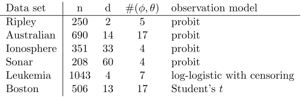
Using several real data sets we present results illustrating the properties of the reviewed LOO-CV approximations. Table 3 lists the basic properties of four classification data sets (Ripley, Australian, Ionosphere, Sonar), one survival data set with censoring (Leukemia), and one data set for a Student’s t regression (Boston). All data sets are available from the internet. Several classification data sets were selected as the posterior is likely to be skewed and there are often differences in performance between Laplace approximation and expectation propagation. The classification data sets have different numbers of covariates so we can investigate to what degree this affects the accuracy of the LOO-CV approximations. The leukemia survival data set was selected as we often analyze survival data with censoring. The Boston data set for a regression with a Student’s tobservation model was selected to illustrate the performance in the case of a non-log-concave likelihood, which may produce multimodal latent posterior. Similar results were obtained with other data sets not reported here.
Data set n d #(φ, θ) observation model
Ripley 250 2 5 probit
Australian 690 14 17 probit
Ionosphere 351 33 4 probit
Sonar 208 60 4 probit
Leukemia 1043 4 7 log-logistic with censoring
Boston 506 13 17 Student’st
Table 3: Summary of data sets and models in our examples.
where we use one common length scale. For the classification data sets we use a Bernoulli observation model with probit link. For the Leukemia data set we use a log-logistic model with censoring (as in Gelman et al., 2013, p. 511). For the Boston data set we use a Student’s tobservation model withν = 4 degrees of freedom. A fixedν was chosen as the Laplace approximation (Vanhatalo et al., 2009) had occasional problems when integrating over an unknownν. Robust-EP by Jyl¨anki et al. (2011) works well also withν unknown. All the experiments were done using GPstuff toolbox1 (Vanhatalo et al., 2013). The Laplace method is implemented as described in Vanhatalo et al. (2010). The Laplace-EM method for Student’st model is implemented as described in Vanhatalo et al. (2009). Parallel EP for other data sets than Boston and parallel robust-EP for Student’st models are implemented as described in Jyl¨anki et al. (2011). CCD is implemented as described in Vanhatalo et al. (2010). Markov chain Monte Carlo (MCMC) sampling is based on elliptical slice sampling for
latent values (Murray et al., 2010) and surrogate slice sampling (Murray and Adams, 2010) for jointly sampling latent values and hyperparameters. The practical speed comparisons of the posterior and LOO approximation methods are shown in Appendix C.
Although in the review we described the estimation of the expected performance LOO =
1 n
Pn
i=1logp(yi|xi, D−i), below we report n×LOO. For these data sets this puts the
approximation errors for all sets on the same scale. This scale has two other interpretations. First, the difference between the sum training log predictive density and n×LOO can be interpreted sometimes as the effective number of parameters measuring the model complexity (Vehtari and Ojanen, 2012; Gelman et al., 2014). Second, the significance of the difference between two models can be approximately calibrated if n×LOO is interpreted as a pseudo log Bayes factor and if a similar calibration scale is used as for the Bayes factor (Vehtari and Ojanen, 2012). As a rule of thumb, based upon asymptotic theory and experience we would like the approximation error fornLOO to be smaller than 1. See the additional discussion of using Bayesian cross-validation in model selection in Vehtari and Lampinen (2002) and Vehtari and Ojanen (2012). We let LOOi ≡logp(yi|xi, D−i) andLOO[i be the corresponding
approximate quantity. In the tables we report a bias and deviation of individual terms as
Bias =
n
X
i=1
(LOO[i−LOOi) (63)
Std2=
n
X
i=1
(LOO[i−LOOi−Bias)2. (64)
The acronyms used in the following are MCMC=Markov chain Monte Carlo, CCD=central composite design, MAP=Type II maximum a posteriori, PSIS=Pareto smoothed importance sampling, and those listed in Tables 1 and 2.
4.1 Exact LOO Comparison to MCMC
The ground truth exact LOO results were obtained by brute force computation of each
p(yi|xi, D−i) separately by leaving out theith observation. We do that for each method:
Laplace, EP and MCMC. MCMC serves as the golden standard for the posterior inference to which we compare Laplace and EP. We show results separately for estimating the predictive performance with and without a global correction (CM2/FACT). As discussed in Section 2.5, only the global corrections produce non-Gaussian predictive distributions for the latent variable ˜f at a new point ˜x. Our main interest is in approximating p(yi|xi, D−i), but we
also show exact LOO results for the conditional p(yi|xi, D−i, φ, θ) with fixed parameters θ, φ, which were obtained by optimizing the marginal posterior p(θ, φ|D) (type II MAP). In this case, LOO-CV is unbiased only conditionally as it does not take into account the effect of the fitting of the parametersθ, φ. However, it is useful to first evaluate the accuracy of approximations forp(yi|xi, D−i, θ, φ), as these can be used with integrated importance
sampling (see Section 3.6) for hierarchical computation of p(yi|xi, D−i).
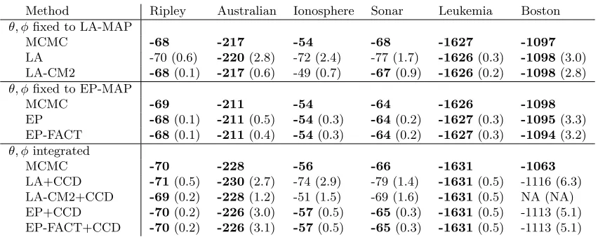
The first part of Table 4 shows the exact LOO results with hyperparameters fixed to Laplace Type II MAP. LA has similar performance to MCMC for all data sets except Ionosphere and Sonar, for which LA is significantly inferior. LA-CM2 is able to improve the predictive performance for the Sonar data set to be similar with MCMC, and for the Ionosphere, the performance is even better than for MCMC.
The second part of Table 4 shows the exact LOO results with hyperparameters fixed to EP Type II MAP. EP has similar performance to MCMC for all data sets and EP-FACT is not able improve the performance. The small differences between MCMC results conditional on either LA-MAP or EP-MAP fixed hyperparameters are due to differences in the marginal likelihood approximations of LA and EP leading to different MAP estimates. However, this difference between LA-MAP and EP-MAP results is less interesting than differences with full integration.
The third part of Table 4 shows the exact LOO results with hyperparameters integrated with MCMC or CCD. LA+CCD is as good as MCMC for the Ripley, Australian and Leukemia data sets. LA-CM2+CCD improves the predictive performance for Ionosphere and Sonar. The performance of LA-CM2+CCD for Sonar is even better than MCMC and EP(-FACT)+CCD. LA-CM2+CCD failed to produce an answer in about 9% of leave-one-out rounds (the LA-CM2 method failing with some hyperparameter values) and thus no result is shown. EP is as good as MCMC for all data sets other than Boston and EP+FACT is not able to improve the performance at all.
Method Ripley Australian Ionosphere Sonar Leukemia Boston θ, φfixed to LA-MAP
MCMC -68 -217 -54 -68 -1627 -1097
LA -70 (0.6) -220(2.8) -72 (2.4) -77 (1.7) -1626(0.3) -1098(3.0)
LA-CM2 -68(0.1) -217(0.6) -49 (0.7) -67(0.9) -1626(0.2) -1098(2.8)
θ, φfixed to EP-MAP
MCMC -69 -211 -54 -64 -1626 -1098
EP -68(0.1) -211(0.5) -54(0.3) -64(0.2) -1627(0.3) -1095(3.3)
EP-FACT -68(0.1) -211(0.4) -54(0.3) -64(0.2) -1627(0.3) -1094(3.2)
θ, φintegrated
MCMC -70 -228 -56 -66 -1631 -1063
LA+CCD -71(0.5) -230(2.7) -74 (2.9) -79 (1.4) -1631(0.5) -1116 (6.3)
LA-CM2+CCD -69(0.2) -228(1.2) -51 (1.5) -69 (1.6) -1631(0.5) NA (NA)
EP+CCD -70(0.2) -226(3.0) -57(0.5) -65(0.3) -1631(0.5) -1113 (5.1)
EP-FACT+CCD -70(0.2) -226(3.1) -57(0.5) -65(0.3) -1631(0.5) -1113 (5.1)
Table 4: Exact LOO (with brute force computation) using MCMC, Laplace (LA), Laplace with CM2 marginal corrections (LA-CM2), EP or EP with FACT marginal correc-tions (EP-FACT) for the latent valuesf, and fixed hyperparameters φ, θ(type II MAP) or integration over the hyperparameters with MCMC or CCD. The values in the parentheses are standard deviations of the pairwise differences from the corresponding MCMC result. Bolded values are not significantly different from the best accuracy in the corresponding category. NA indicates failed computation.
full MCMC is able to find better hyperparameters during the joint sampling of the latent values and hyperparameters.
4.2 Approximate LOO Comparison to Exact LOO – Fixed Hyperparameters
As discussed in Section 3.2, we compute LOO densities p(yi|xi, D−i) hierarchically by first
computing the conditional LOO densities p(yi|xi, D−i, θ, φ). As the accuracy of the full
LOO densities depends crucially on the conditional LOO densities, we first analyze the LOO approximations conditional on fixed hyperparameters. The ground truth in this section are the LA, LA-CM2, EP, and EP-FACT results shown in Table 4.
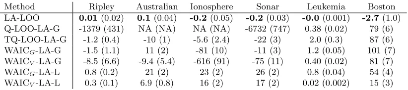
Table 5 shows results when the ground truth is exact LOO with fixed parameters and Laplace approximation without a global correction (LA in Table 4). LA-LOO gives the best accuracy for all data sets by a significant margin. Quadrature LOO with Gaussian approximation of the latent marginals (Q-LOO-LA-G) produces bad results for the clas-sification data sets and sometimes completely fails. The posterior marginals in the case of the Leukemia model are so close to Gaussian that Q-LOO-LA-G also provides a useful result. Truncated quadrature (TQ-LA-LOO-G) is more stable, but it cannot fix the whole problem. Using more accurate marginal approximation improves WAICs. WAICV with the
LA-L marginal approximation gives useful results for the two simplest data sets.
Method Ripley Australian Ionosphere Sonar Leukemia Boston
LA-LOO 0.01(0.02) 0.1(0.04) -0.2(0.05) -0.2(0.03) -0.0(0.001) -2.7(1.0)
Q-LOO-LA-G -1379 (431) NA (NA) NA (NA) -6732 (747) 0.38 (0.02) 79 (6)
TQ-LOO-LA-G -1.2 (0.4) -10 (1) -5.6 (2.4) -22 (3) 2.0 (0.3) 87 (6)
WAICG-LA-G -1.5 (1.1) 11 (2) -81 (10) -11 (3) 1.2 (0.05) 101 (7)
WAICV-LA-G -8.5 (6.6) -9.4 (5.4) -616 (91) -75 (11) 0.40 (0.02) 81 (7)
WAICG-LA-L 0.8 (0.2) 21 (2) 23 (2) 26 (2) 0.8 (0.04) 54 (4)
WAICV-LA-L 0.3 (0.1) 6.9 (0.8) 16 (2) 17 (2) 0.02 (0.002) 15 (3)
Table 5: Bias and standard deviation when the ground truth is exact LOO with Laplace and fixed full posterior MAP hyperparameters (LA in Table 4). Bolded values have significantly smaller absolute value than the values from the other methods for the same data set. NA indicates that computation failed.
Method Ripley Australian Ionosphere Sonar Leukemia Boston
EP-LOO 0.2(0.1) 1.6(0.5) 0.3(0.4) -0.5(0.1) -0.0(0.003) -1.1(0.9)
Q-LOO-EP-G -352 (171) NA (NA) NA (NA) NA (NA) 0.02 (0.003) 33 (3)
TQ-LOO-EP-G -0.2 (0.2) 14 (8) 20 (4) NA (NA) 1.7 (0.4) 44 (4)
WAICG-EP-G 0.7 (0.2) 59 (8) 0.5(3) -42 (4) 0.8 (0.04) 76 (5)
WAICV-EP-G -0.2 (0.4) -4.3 (7) -94 (11) -804 (64) 0.03 (0.004) 37 (3)
WAICG-EP-L 0.7 (0.2) 81 (8) 23 (3) 48 (4) 0.8 (0.04) 81 (5)
WAICV-EP-L 0.4 (0.1) 54 (6) 17 (2) 42 (4) 0.02 (0.003) 26 (3)
Table 6: Bias and standard deviation when the ground truth is exact LOO with EP and fixed full posterior MAP hyperparameters (EP in Table 4). Bolded values have significantly smaller absolute values than the values from the other methods for the same data set. NA indicates that computation failed.
and Leukemia data sets are easy enough for most of the methods to produce useful accuracy.
Table 7 shows results when the ground truth is exact LOO with fixed parameters and Laplace approximation with LA-CM2 global correction (LA-CM2 in Table 4). Quadrature LOO with LA-CM2 approximation of the latent marginals (Q-LOO-LA-CM2) has the best accuracy for all data sets except for Boston, but the accuracy is satisfactory only for the Ripley and Leukemia data sets. Here LA-LOO has a negative bias as the global correction LA-CM2 can improve the marginal approximation and therefore also the expected performance estimated with exact LOO. The results for truncated quadrature (TQ-LOO-LA-CM2) are not reported in the table as with adaptive truncation it produced the same results as quadrature LOO (Q-LOO-LA-CM2). WAICV performs better than WAICG, but
worse than Q-LOO-LA-CM2.
Method Ripley Australian Ionosphere Sonar Leukemia Boston
LA-LOO -1.4 (0.6) -3.3 (3.3) -23 (3) -11 (2) 0.00(0.1) -2.6(2.2)
Q-LOO-LA-CM2 0.3(0.1) 3.1(0.5) 9.0(1.8) 7.4(0.9) 0.01(0.0004) 11 (2)
WAICG-LA-CM2 1.0 (0.2) 25 (3) 16 (3) 27 (3) 0.8 (0.04) 61 (4)
WAICV-LA-CM2 0.5 (0.1) 11 (2) 13 (2) 20 (3) 0.02 (0.002) 22 (3)
Table 7: Bias and standard deviation when the ground truth is exact LOO with Laplace-CM2 and fixed full posterior MAP hyperparameters (LA+Laplace-CM2 in Table 4). Bolded values have significantly smaller absolute values than the values from the other methods for the same data set.
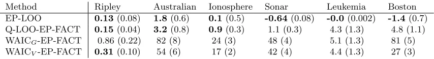
Method Ripley Australian Ionosphere Sonar Leukemia Boston
EP-LOO 0.13(0.08) 1.8(0.6) 0.1(0.5) -0.64(0.08) -0.0(0.002) -1.4(0.7)
Q-LOO-EP-FACT 0.15(0.04) 3.2(0.8) 0.9(0.3) 1.1 (0.3) 4.3 (1.3) 4.8 (1.1)
WAICG-EP-FACT 0.86 (0.22) 82 (8) 24 (3) 48 (4) 5.1 (1.3) 81 (5)
WAICV-EP-FACT 0.31(0.10) 54 (6) 17 (2) 42 (4) 4.4 (1.3) 27 (3)
Table 8: Bias and standard deviation when the ground truth is exact LOO with EP-FACT and fixed full posterior MAP hyperparameters (EP+FACT in Table 4). Bolded values have significantly smaller absolute values than the values from the other methods for the same data set.
results. The EP-LOO using the EP-L tilted distribution approximation is already good and the global correction does not change the result much. Small errors in the quadrature integration cumulate and Q-LOO-EP-FACT produces slightly worse results than EP-LOO.
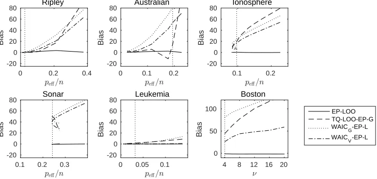
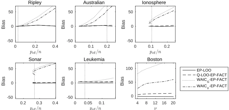
4.3 LOO and WAIC with Varying Model Flexibility
Above we saw that the methods other than LA-LOO and EP-LOO had more difficulties with most of the data sets and especially with data sets with a large number of covariates. Figures 1–4 illustrate how the flexibility of the Gaussian process models affects the performance of the approximations. We took the models with MAP parameter values and re-ran the models and LOO tests, varying the length scales for all data sets except Boston (see later). With a smaller length scale, the GPs are more flexible and more non-linear. With a larger length scale GPs approach the linear model. We measure the flexibility by the difference between the mean training log predictive density and LOO, which can be interpreted as the degree to which the model has fit to the data or the relative effective number of parameters (peff/n).
When the length scale gets smaller, there will be more such fis that have a low correlation
with any other fj. In this case the full marginal posterior and LOO marginal posterior
rule of thumb, methods other than LA-LOO and EP-LOO start to fail when the relative effective number of parameters (peff/n) is larger than 2%–5%.
Figures 1–4 also show for Boston data how the degrees of freedom ν in the Student’st
observation model affects the accuracy. When ν increases, the observation model is closer to Gaussian and the latent posterior is more likely to be unimodal. Although the latent posterior is easier to approximate with a Gaussian when ν is large, the posterior is less robust to influential observations (“outliers”) and the error made by the methods other than LA-LOO and EP-LOO increases.
4.4 Approximate LOO Comparison to Exact LOO – Hierarchical Model
Next we examine the accuracy of hierarchical LOO approximation of p(yi|xi, D−i) (see
Section 3.2), where the conditional LOO densities p(yi|xi, D−i, θ, φ) are approximated with
LA-LOO or EP-LOO, which we found performed best for conditional densities (see previous section).
Table 9 shows the results whenthe ground truth is exact LOO with CCD used to integrate over the parameter posterior and the Laplace method is used to integrate over the latent values
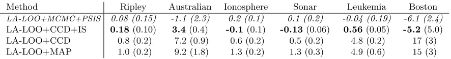
(LA+CCD in Table 4). The Laplace approximation combined with type II MAP parameter estimates or CCD integration but no importance weighting has an error size related to the number of hyperparameters (θ, φ). The unweighted CCD or MAP gives a small error only if the number of parameters (θ, φ) is small. Importance weighting of CCD works well for all data sets except Australian and Boston. These data sets have more parameters (17) than the others (4-8), making the inference more difficult. The minimum relative effective sample sizes (Ripley=60%, Australian=16%, Ionosphere=59%, Sonar=70%, Leukemia=36%, Boston=0.3%) correctly indicate that importance weighting for Australian and Boston data sets is unreliable.
Table 10 shows the corresponding results when the ground truth is exact LOO with CCD used to integrate over the parameter posterior and expectation propagation used to integrate over the latent values (EP+CCD in Table 4). EP with the unweighted CCD or MAP gives a small error only if the number of parameters (θ, φ) is small. Importance weighting of CCD works well for all data sets except Australian and Boston. Again the minimum relative effective sample sizes (Ripley=60%, Australian=12%, Ionosphere=36%, Sonar=65%, Leukemia=35%, Boston=9%) correctly indicate that importance weighting for Australian and Boston is unreliable.
pe,=n
0 0.2 0.4
Bias -20 0 20 40 60 80 Ripley
pe,=n
0 0.1 0.2
Bias -20 0 20 40 60 80 Australian
pe,=n
0.1 0.2 Bias -20 0 20 40 60 80 Ionosphere
pe,=n 0.1 0.2 0.3
Bias -20 0 20 40 60 80 Sonar
pe,=n 0 0.05 0.1
Bias -20 0 20 40 60 80 Leukemia 8
4 8 12 16 20
Bias 0 50 100 Boston LA-LOO TQ-LOO-LA-G WAIC G-LA-L
WAICV-LA-L
Figure 1: Bias when the ground truth is exact LOO with Laplace (LA in Table4) and varying flexibility of the model, or degrees of freedom in the Student’st model for the Boston data. Model flexibility was varied by rescaling the length scale(s) in the GP model. Model flexibility is measured by the relative effective number of parameterspeff/n. The flexibility of the MAP model is shown with a vertical
dashed line. For the Student’st model the vertical dashed line is atν= 4.
pe,=n
0 0.2 0.4
Bias -20 0 20 40 60 80 Ripley
pe,=n
0 0.1 0.2
Bias -20 0 20 40 60 80 Australian
pe,=n
0.1 0.2 Bias -20 0 20 40 60 80 Ionosphere
pe,=n 0.1 0.2 0.3
Bias -20 0 20 40 60 80 Sonar
pe,=n 0 0.05 0.1
Bias -20 0 20 40 60 80 Leukemia 8
4 8 12 16 20
Bias 0 50 100 Boston EP-LOO TQ-LOO-EP-G WAICG-EP-L
WAICV-EP-L
Figure 2: Bias when the ground truth is exact LOO with EP (EP in Table4) and varying flexibility of the model, or degrees of freedom in the Student’s t model for the Boston data. Model flexibility was varied by rescaling the length scale(s) in the GP model. Model flexibility is measured by the relative effective number of parameters
peff/n. The flexibility of the MAP model is shown with a vertical dashed line. For
pe,=n
0 0.2 0.4
Bias
-50 0 50
Ripley
pe,=n
0 0.1 0.2
Bias
-50 0 50
Australian
pe,=n
0 0.1 0.2
Bias
-50 0 50
Ionosphere
pe,=n
0.2 0.3 0.4
Bias
-50 0 50
Sonar
pe,=n 0 0.05 0.1
Bias -50 0 50 Leukemia 8
4 8 12 16 20
Bias 0 50 100 Boston LA-LOO Q-LOO-LA-CM2 WAIC G-LA-CM2
WAICV-LA-CM2
Figure 3: Bias when the ground truth is exact LOO with Laplace-CM2 (LA-CM2 in Table4) and varying flexibility of the model, or degrees of freedom in the Student’stmodel for the Boston data. Model flexibility was varied by rescaling the length scale(s) in the GP model. Model flexibility is measured by the relative effective number of parameterspeff/n. The flexibility of the MAP model is shown with a vertical
dashed line. For the Student’st the vertical dashed line is atν = 4.
pe,=n
0 0.2 0.4
Bias
-50 0 50
Ripley
pe,=n
0 0.1 0.2
Bias
-50 0 50
Australian
pe,=n
0 0.1 0.2
Bias
-50 0 50
Ionosphere
pe,=n
0.2 0.3 0.4
Bias
-50 0 50
Sonar
pe,=n 0 0.05 0.1
Bias -50 0 50 Leukemia 8
4 8 12 16 20
Bias 0 50 100 Boston EP-LOO Q-LOO-EP-FACT WAIC G-EP-FACT
WAICV-EP-FACT
Figure 4: Bias when the ground truth is exact LOO with EP-FACT (EP-FACT in Table4) and varying flexibility of the model, or degrees of freedom in the Student’stmodel for the Boston data. Model flexibility was varied by rescaling the length scale(s) in the GP model. Model flexibility is measured by the relative effective number of parameterspeff/n. The flexibility of the MAP model is shown with a vertical
Method Ripley Australian Ionosphere Sonar Leukemia Boston LA-LOO+MCMC+PSIS 0.08 (0.15) -1.1 (2.3) 0.2 (0.1) 0.1 (0.2) -0.04 (0.19) -6.1 (2.4)
LA-LOO+CCD+IS 0.18(0.10) 3.4(0.4) -0.1(0.1) -0.13(0.06) 0.56(0.05) -5.2(5.0)
LA-LOO+CCD 0.8 (0.2) 7.2 (0.9) 0.6 (0.2) 0.5 (0.2) 4.8 (0.2) 17 (3)
LA-LOO+MAP 1.0 (0.2) 9.2 (1.8) 1.3 (0.2) 1.3 (0.3) 4.9 (0.6) 15 (3)
Table 9: Bias and standard deviation when the ground truth is exact LOO with Laplace and CCD (LA+CCD in Table 4). Bolded values have significantly smaller absolute error than the values from the other methods for the same data set.
Method Ripley Australian Ionosphere Sonar Leukemia Boston
EP-LOO+MCMC+PSIS 0.38 (0.17) -2.4 (3.4) 0.8 (0.5) -0.23 (0.22) -0.16 (0.23) -0.9 (1.0)
EP-LOO+CCD+IS 0.42(0.14) 7.3(1.4) 0.8(0.6) -0.24(0.14) 0.49(0.04) 2.2(1.0)
EP-LOO+CCD 1.3 (0.4) 15 (2) 2.8 (1.3) 0.6 (0.3) 4.8 (0.2) 20 (2)
EP-LOO+MAP 1.4 (0.3) 17 (2) 2.8 (0.7) 0.9 (0.3) 4.9 (0.6) 17 (2)
Table 10: Bias and standard deviation when the ground truth is exact LOO with EP and CCD (EP+CCD in Table 4). Bolded values have significantly smaller absolute error than the values from the other methods for the same data set.
If the minimum relative effective sample size or PSIS diagnostics warn about potential problems, depending on the application it may be necessary to run, for example, k-fold cross-validation.
5. Discussion
We have shown that LA-LOO and EP-LOO provide fast and accurate conditional LOO results when the predictions at new points are made using the Gaussian latent value distribution. If the predictions at new points are made using non-Gaussian distributions obtained from the global correction, then quadrature LOO gives useful results, but it would be faster and more accurate to just use EP without the global correction. Both Laplace-LOO and EP-LOO can be combined with importance sampling or importance weighted CCD to get fast and accurate full Bayesian leave-one-out cross-validation results.
If other methods than LA-LOO or EP-LOO are used, we propose the following rule of thumb for diagnostics: The methods other than LA-LOO and EP-LOO start to fail when the relative effective number of parameters (peff/n) is larger than 2%–5%.
Here we have considered fully factorizing likelihoods, but the methods can be extended for use with likelihoods with grouped factorization, such as in multi-class classification, multi-output regression, and some hierarchical models with lowest level grouping. We assume that the accuracy using Laplace-LOO and EP-LOO would also be good in these cases.